www.nonlin-processes-geophys.net/18/269/2011/ doi:10.5194/npg-18-269-2011
© Author(s) 2011. CC Attribution 3.0 License.
Nonlinear Processes
in Geophysics
Using a variance-based sensitivity analysis for analyzing the relation
between measurements and unknown parameters of a physical
model
J. Zhao and C. Tiede
Department of Geoinformatics, University of Applied Sciences Munich, Karlstr. 6, 80333 Munich, Germany Received: 6 December 2010 – Revised: 8 April 2011 – Accepted: 20 April 2011 – Published: 3 May 2011
Abstract. An implementation of uncertainty analysis (UA) and quantitative global sensitivity analysis (SA) is applied to the non-linear inversion of gravity changes and three-dimensional displacement data which were measured in and active volcanic area. A didactic example is included to il-lustrate the computational procedure. The main emphasis is placed on the problem of extended Fourier amplitude tivity test (E-FAST). This method produces the total sensi-tivity indices (TSIs), so that all interactions between the un-known input parameters are taken into account. The possible correlations between the output an the input parameters can be evaluated by uncertainty analysis. Uncertainty analysis re-sults indicate the general fit between the physical model and the measurements. Results of the sensitivity analysis show quite different sensitivities for the measured changes as they relate to the unknown parameters of a physical model for an elastic-gravitational source. Assuming a fixed number of ex-ecutions, thirty different seeds are observed to determine the stability of this method.
1 Introduction
In Moldwin and Rose (2009), the majority of the articles sur-veyed did not discuss measurement uncertainty or present er-ror bars in observational or statistical analysis figures. We conducted a survey of 31 articles published between 2005 and 2010 having “sensitivity analysis” as a keyword using American Geophysical Union (AGU) Earth and Space In-dex (EASI) search engine. The majority (21) applied the sensitivity analysis practices to hydrology. The application of SAs can be exiguously found in the modeling of various branches of geodesy, e.g. non-linear geodetic data inversion
Correspondence to: J. Zhao ([email protected])
(Tiede et al., 2005), model evaluation in engineering survey (Schwieger, 2004), and model optimization for trajectory es-timation (Schwieger, 2006).
The study of uncertainty is usually composed of two re-lated activities referred as uncertainty analysis and sensitivity analysis. Uncertainty analysis aims quantifying the overall uncertainty associated with the response as a result of un-certainties in the model input. Ideally, SA and UA should be computed in tandem, with UA preceding in current prac-tice. SA is a study of how uncertainty in the output of a model (numerical or otherwise) can be apportioned, qualita-tively or quantitaqualita-tively, to different sources of uncertainty in the model input, and of how the given model depends upon the information fed into it, (Saltelli et al., 2000, 2008). It can be seen as a tool for validating and optimizing a model due to the determination of the sensitivities of the different output values concerning changes in the unknown input parameters. This knowledge results in the quantification as well as the qualification of the unknown input parameters, so it can be derived which parameter has to be known best in order to re-duce the variance of a certain output value. In geodesy mea-surement models, the inputs are the meamea-surement quantities and the outputs are the corrected or reduced measurements, the estimated coordinates or other parameters. SA studies the relationship between input and output quantities of the model (Schwieger, 2006).
Sensitivity analysis of model output examines how a model depends on its input parameters. Two groups of sen-sitivity analyses are defined: local sensen-sitivity analysis and global sensitivity analysis (Saltelli et al., 2000). One draw-back of local SA is that it is not possible to quantify the ef-fects caused by the interactions between the unknown input parameters. Thus, we are using global SA techniques instead of local SA.
strongly favor those capable of computing the so-called “To-tal Sensitivity Indices” (TSI), which measures a parameter’s main effect and all the interactions involving that parameter, especially since the analyst cannot know in advance whether his/her model will be additive in all its factors (Saltelli et al., 2000).
Due to the lack of knowledge if the underlying physical based mathematical model is additive or not, and its non-linear behavior, a variance-based, global sensitivity analy-sis which can also compute the interactions between the un-known parameters has been chosen. Because the number of unknown input parameters is very small with an amount of five (X=[ξ, ψ, ζ, , m]), (details on the parameters are dis-cussed in Sect. 2) the aspect of computation time for the anal-ysis is negligible for the choice of the method. From the two variance-based global techniques which allow the computa-tion of TSIs, as Sobol’ has been discussed in Tiede (2005) and Tiede et al. (2005), Extended Fourier Amplitude Sensi-tivity Test (E-FAST) has been applied. E-FAST – an evolu-tion of FAST – is a variance-based SA technique among the methods most used. It was proposed to combine FAST better efficiency with Sobol’ capacity to compute total effects by Saltelli et al. (1999). The current paper gives an assessment of this method applied to a geodetic model.
2 Case study Merapi volcano
As a case study, gravity changes (dg) and three-dimensional displacements (dx, dy and dz) were measured at different time epochs in a permanently active area around Merapi vol-cano located at Java, Indonesia. One possible explanation for the measured changes in gravity and three-dimensional displacements is given by a changing status of the magma chamber of the volcano happened within the time period be-tween measurement epocht andt+1. Such a status change of the magma chamber can be produced by a change in its position, mass and its energy change of the intrusion which all would cause signals at the surface that can be measured by different sensors like GPS and gravitymeters.
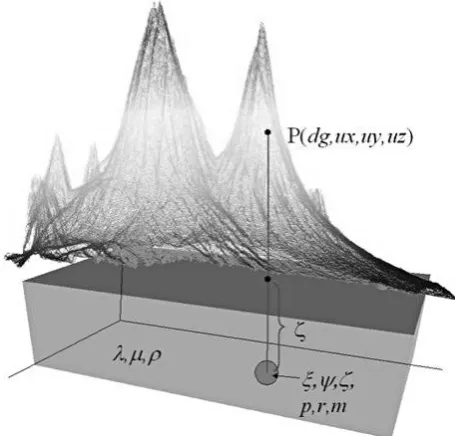
Figure 1 describes the model,whereby the unknown pa-rameters of the model are given by its position (the east co-ordinate (ξ), the north coordinate (ψ) and the depth (ζ)), the mass (m) and the energy of the intrusion () described by the product of pressure (p) and cubed radius (r). Table 1 shows the boundaries of the unknown input parameters. The pa-rameters of the magma chamber are estimated by the model in Eq. (2) using gravity changes (dg), height displacements (uz), east displacements (ux) and north displacements (uy) at about 20 observation points arranged in a loop based net-work structure around the volcano.
The used forward model for estimating the unknown pa-rameters of the source is based on the generalized static Navier equations which couple elastic and gravitational ef-fects in a homogeneous half space, given by Love (1911) and Rundle (1980).
Fig. 1. Elastic-gravitational model (Tiede, 2005).
Table 1. Range limitations for the input parameters used for the computation.
Unknown input parameter Lower bound Upper bound
Eastξ(103m) 37 41
Northψ(103m) 65 68
Heightζ(103m) 0.01 0.5
Energy(1014N·m) 0 800
Massm(1012kg) 0.01 0.5
0= ∇2u+ 1
1−2σ∇∇ ·u+ ρ0g
µ ∇(u·ez) (1)
−ρ0
µ∇φ− ρ0g
µ ez∇ ·u
∇2φ=4πρ0G∇ ·u
For the purpose of this inversion the values which describe the medium of the subsurface are given by the Poisson’s ratio σ, chosen as 0.25 for an elastic medium. The Young’s mod-ulusE was considered to be 30 GPa, according to Beaudu-cel et al. (2000). The mean density for this area is given as 2242 kg m−3, a value which was derived by gravity data in-version for the area of interest (Tiede et al., 2005).
For the computation of the most probable values of the unknown parameters a global optimization technique such as genetic algorithm (GA) has been used (Tiede, 2005), which maximizes the objective function that is given as the χ2 value. For the estimation of the unknown parameters of Eq. (2), the objective functionχ (comp)2(“comp” stands for “complete”) is computed by taking all kind of changes: grav-ity changes as well as the three-dimensional displacements into account, Eq. (2).
χ (comp)2=v
T Q−1v
n−u (2)
withnas number of all observations (here 80), u as num-ber of unknown model parameters (here 5),v as the vector of residuals between modeled and measured values andQ
as covariance matrix holding the variances of the measured values on its diagonal. Within the generated sensitivity anal-yses, Sect. 4, we use additional objective functionsχ (dg)2, χ (ux)2,χ (uy)2, andχ (uz)2(based on Eq. (2) but only com-puted via gravity changes, east, north and height displace-ments separately). The objective functions are computed by the kind of observation which is given in brackets.
Table 2 presents the observed changes in eastux, northuy, heightuzand gravitydg, including their mean standard de-viationsσ¯ of 20 points. Due to the small standard deviations of the measurements we just take the standard deviations into account as weights in the computation of the objective func-tions. But generally we do not compute an uncertainty ana-lysis based on observational uncertainties here. It could be discussed in a subsequent paper.
3 Methods
3.1 Uncertainty analysis
The uncertainty of measurement is a parameter, associated with the result of a measurement, that characterizes the dis-persion of the values that could reasonably be attributed to the measurand (GUM, 2008). In geodesy measurement, there are a number of sources of uncertainty, which include: parameter randomness due to geodetic processes; the lack of dense spatial measurements of geodetic parameters; un-certainty due to incomplete historical geodetic data collec-tion, data measurement error, and unpredictability of future geodetic events; and model uncertainty attributed to the lim-itation of a simulation model to correctly represent the phys-ical processes of the system.
Table 2. Observation changes of the points including the mean stan-dard deviations.
Maximum Minimum σ¯
ux(cm) 21.9 −3.3 0.4
uy(cm) 58.4 −18.6 0.3
uz(cm) 25.7 −11.5 2.4
dg(mGal) 0.149 −0.048 0.012
UA refers to the determination of the uncertainty in ana-lysis results that derives from uncertainty in anaana-lysis input. Important components of uncertainty analysis include qual-itative analysis that identifies the uncertainties, quantqual-itative analysis of the effects of the uncertainties on the decision process, and communication of the uncertainty. The analysis of the uncertainty depends on the problem.
The approach for assessing parameter uncertainty involves the following steps, in Smith (2002):
1. Select a distribution to describe possible values of a pa-rameter.
2. Generate data from this distribution.
3. Use the generated data as possible values of the param-eter in the model to produce output.
3.2 Variance-based Extended Fourier Amplitude Sensitivity Test (E-FAST) SA
The main idea of variance-based global sensitivity analyses is based on the idea that one can determine the nature of the sensitivity through the varianceV and then evaluate how the input variance contributes to the output variance. By setting (X1, ..., Xk)as the vector of independent unknown input pa-rameters andY =f (X1, ..., Xk)as the output value, with f as model function, an indicator for the importance of an inputXi can be set by evaluating the variance of the output Y V (Y|Xi). This is done by fixingXito a valuexi.V (Y|Xi) is called the conditional variance ofY withXi=xi. The true value ofxi is not known, so instead ofV (Y|Xi)the expec-tation of the conditional variance, noted asE[V (Y|Xi)] is studied, whereby it is built into all possible values ofxi. The variance ofY is given by
Si as the ratio between the variance of the expectation value and the variance of the output value leads to
Si=
V (E[Y|Xi])
V (Y ) (4)
and is called the first order sensitivity index, correlation ratio or importance measure and describes the main effect of the unknown parameterXion the output valueY.
Related to Confalonieri et al. (2010), the total sensitivity index (TSI) corresponding to a single factor (indexi) and the interaction of more factors that involve the indexiand at least one indexj6=ifrom 1 ton:
STi= X
Si+ X
j6=i
Sij+...+S1...n (5)
Both the main effects Si, the interaction terms Sij and higher-order terms could be computed by straightforward Monte-Carlo integration of multidimensional integrals. The main effect (or first order) sensitivity index measures only the main effect contribution of each input parameter on the out-put variance. The interactions among the inout-put parameters are not taken into account. If the total effect on the output of input parameters is not equal to the sum of their first order effects is called interact. A model with interactions is said to be non-additive. For non-additive models information from all interactions is searched for, as well as the first order effect. For nonlinear models the sum of all first order indices can be very low. The sum of all the order effects that a parameter accounts for is called the total effect. So, for an inputXi, the total sensitivity index STi(Eq. 5) is defined as the sum of all indices relating toXi (first and higher orders).
The classical FAST method, created in the 1970s by Cukier, Schaibly and others, and further developed by Koda and McRae, estimates the first-order effects. Saltelli et al. (1999) propose the E-FAST method, which computes both first-order effects and total effects. The term total means the factor’s main effect and all the interaction terms of that factor. The main advantages of the E-FAST is pointed out in Saltelli et al. (1999) is that it allows the simultaneous computation of the first and total effect indices for a given factor. And it is robust at low sample size and computational efficient.
The main idea of the FAST method is to convert the mul-tidimensional integral inX into a one-dimensional integral insby using the transformation functionsXi=Gi(sinωis) for i=1, ..., k. s∈(−π,π ) is a scalar variable and ωi is a set of integer angular frequencies. The basic idea behind the computation of the total indices by the FAST method is to consider the frequencies that do not belong to the set {p1ω1,p2ω2,...,pkωk}, for pi =1,2,...,∞ and
∀i=1,2,...,k. These frequencies contain information about the residual varianceV−Pk
iVi that is not accounted for by the first-order indices, that is, including the interactions be-tween the factors at any order.
We assign a frequencyωi for the factor Xi and a set of almost identical frequencies, but different fromωi, to all the
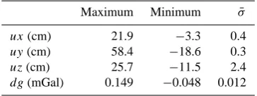
Fig. 2.χ (comp)2distribution against the east componentξrelative to the 28 645 Monte Carlo samples.
remaining factors, denoted byω∼i. We use∼ito represent “all buti”. The chosen frequencies and their harmonics have to be linear independent. Thus, by evaluating the spectrum at the frequenciesω∼iand related higher harmonicspωi, we can compute the partial varianceV∼i. V∼i is a measure in-cluding all the effects of any orders that do not involve the factorXi. The total index, denoted by TS(i), is computed by using the following equation
TS(i)=1−V∼i
V (6)
4 Results
4.1 Uncertainty analysis
In this case, the probability density functions (pdfs) of the unknown input parameters had been anticipated as uniform because it has not been possible to specify any areas or cer-tain value ranges which are more likely than others within the given limits for the unknown input parameters given in Table 1. Furthermore, in cases with only poor prior knowl-edge of the unknown input parameters pdfs, Saltelli et al. (2000) also suggests a unique distribution.
Fig. 3.χ (comp)2distribution against the mass componentm rela-tive to the 28 645 Monte Carlo samples.
Furthermore, the distributions of the uncertainty plots are analyzed: Analyzing the distribution of χ (comp)2 in Fig. 2, high values can be observed for east components ξ 37·103≤ξ≤37.8·103m as well as one more region 38.5·103≤ξ≤40·103m which show large variance in the objective function. Large values indicate a large value of the objective function which implies a bad fit between measured data and physical model. Taking the range ofξ where the small values ofχ (comp)2appear (37.8·103≤ξ≤38.5·103 or 40·103≤ξ ≤41·103 ) for analysis leads to better fit between measurements and model. As shown in Fig. 3, the values of the χ (comp)2 follow a homogeneous distri-bution over the range of mass component m values. The χ (comp)2can be seen as the sum of the four objective func-tionsχ (dg)2, χ (ux)2, χ (uy)2 andχ (uz)2. The effect of the mass component is overlapping, so no clear behavior can be determined out in this plot. Nevertheless, the distribu-tion ofχ (dg)2(see Fig. 4) against mass componentmshows small value ofχ (dg)2for smallm. The dispersion is increas-ing with enlargincreas-ingm. The analysis of the relation between χ (dg)2and the the mass component mresults in a region 0≤m≤0.15·1012kg. This small dispersion together with small values of the objective function state that small mass values explain the measurements at best.
4.2 Variance-based Extended Fourier Amplitude Sensitivity Test (E-FAST) SA
The previous discussed results show first relations between unknown input parameters and the output values and will be analyzed in more detail by applying the E-FAST variance-based sensitivity analysis. Therefore, the first order effects as well as the TSIs are computed after Sect. 3.2 for all five
Fig. 4.χ (dg)2distribution against the mass componentmrelative to the 28 645 Monte Carlo samples.
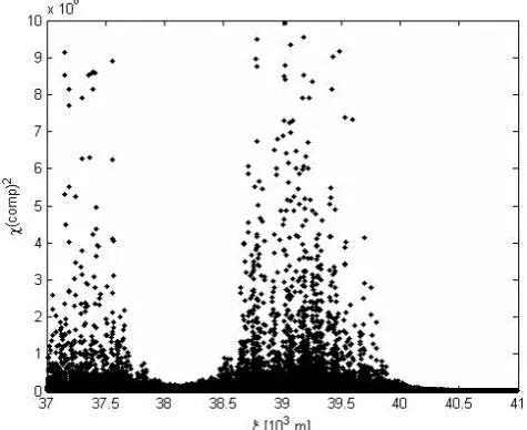
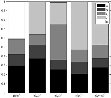
Fig. 5. First order effects and TSIs computed by E-FAST sensi-tivity analysis for the Monte Carlo sampling (one run consisting of 28 645 samples).
Fig. 6. Normalized E-FAST first order indices for the five defined output parameters (one run consisting of 28 645 samples).
It indicates that all TSIs are driven primarily by interactions between the input parameters.
Figures 6 and 7 display the normalized E-FAST first order indices and TSIs with respect to the un-known input parameters for all kind of output val-ues (χ (dg)2,χ (uz)2,χ (ux)2,χ (uy)2,χ (comp)2) separately. The normalization is investigated according to
S()n,i =S()i/ 5 X
i=1
S()i (7)
TSI()n,i =TSI()i/ 5 X
i=1
TSI()i (8)
withS()n,i = normalized first order sensitivity index of the values given in the brackets due to the specified unknown in-put parameteri,S()i= first order sensitivity index concern-ing the unknown input parameter i, TSI()n,i= normalized TSI due to the unknown input parameteriand TSI()i= total sensitivity index due to the unknown input parameteri.
The obvious changes in sensitivity indices in Figs. 6 and 7 caused by higher order effects confirm the described results in Fig. 5.
By analyzing the E-FAST TSIs, the influences on the ob-served values due to the unknown input parameters are obvi-ous. All output values are almost equally sensitive to changes in the three location parameters (ξ,ψ, andζ). The three lo-cation parameters of the source have similar influences (ap-proximately 25 %) on these output values. The mass m has only few influence (below 5 %) on the output values except χ (dg)2values (15 %). The energy effect, by contrast, has similar influences (around 15 %) on the output values except χ (dg)2values (6 %).
Fig. 7. Normalized E-FAST Total Sensitivity Indices (TSI) for the five defined output parameters (one run consisting of 28 645 sam-ples).
Table 3. Nonnormalized E-FAST TSIs for the five defined output
parameters with respect to the height componentζ with 4 different
seeds (1, 500, 4000, 10 000) and the mean TSIs of 30 executions (the standard deviation see Table 6 row 3).
Output value Seed Mean
1 500 4000 10 000
χ (dg)2 0.7610 0.8260 0.8288 0.8026 0.8124
χ (uz)2 0.8514 0.7861 0.8546 0.8659 0.8210
χ (ux)2 0.8624 0.8383 0.8696 0.8739 0.8559
χ (uy)2 0.8579 0.8689 0.8185 0.8685 0.8555
χ (comp)2 0.8568 0.8580 0.8590 0.8728 0.8593
From the sensitivity analysis concerning all χ2 values, conclusions about the estimation of the unknown input pa-rameters can be drawn from Fig. 7:
– The mass componentm can be computed most effec-tively byχ (dg)2due to its large influence on this out-put value. The observations of gravity changes are most important for the determination ofm.
– For the estimation of the energy effect all the output values are appropriate exceptχ (dg)2.
– The three location parameters east componentξ, north componentψ, and height componentζ are good to be estimated by all the measurement.
Table 4. Nonnormalized E-FAST TSIs for the five defined output
parameters with respect to the mass componentmwith 4 different
seeds (1, 500, 4000, 10 000) and the mean TSIs of 30 executions (the standard deviation see Table 6 row 5).
Output value Seed Mean
1 500 4000 10 000
χ (dg)2 0.6430 0.8433 0.5266 0.6145 0.6352
χ (uz)2 0.4553 0.5463 0.3891 0.5504 0.4658
χ (ux)2 0.2294 0.5586 0.3261 0.4641 0.4701
χ (uy)2 0.3543 0.4726 0.3012 0.4078 0.3828
χ (comp)2 0.2183 0.6112 0.2093 0.3223 0.3795
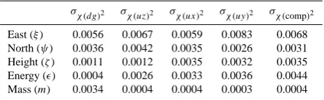
Table 5. Standard deviation of nonnormalized E-FAST first order indices with 30 different seeds.
σχ (dg)2 σχ (uz)2 σχ (ux)2 σχ (uy)2 σχ (comp)2
East (ξ) 0.0056 0.0067 0.0059 0.0083 0.0068 North (ψ) 0.0036 0.0042 0.0035 0.0026 0.0031 Height (ζ) 0.0011 0.0012 0.0035 0.0032 0.0035 Energy () 0.0004 0.0026 0.0033 0.0036 0.0044 Mass (m) 0.0034 0.0004 0.0004 0.0003 0.0004
nonnormalized TSIs for the output parameters with respect to the height componentζ and the mean TSIs of 30 execu-tions. These 4 different seeds are chosen from 1 to 10 000 randomly. The height component has similar influences on all the outputs with different seeds. In contrast, the discrep-ancies between the TSIs with respect to the mass component m(see Table 4) are much greater. The mass component al-ways has largest influence on theχ (dg)2.
The standard deviations of the nonnormalized first order indices in Table 5 are much smaller than for the nonnormal-ized TSIs in Table 6. Furthermore, the TSIs of the east, north and height components are much stabler than that of the en-ergy and mass components. The nonsignificant standard de-viations of the three position parameters (east, north, and height) due to the use of different seeds become in fact neg-ligible which shows that the sample size is large enough for these parameters. But the analysis of the energy and mass is impossible here. In consequence, we try to fix the east, north, and height components and do the SA again just taking the energy and mass as the input parameters.
5 Conclusions
The paper evaluates E-FAST variance-based UA and SA ap-plied for geodetic data in order to determine a deeper insight into the behavior between the unknown input parameters of the physical based mathematical model and the modeled out-put values. The application of UA presents the general fit
Table 6. Standard deviation of nonnormalized E-FAST TSIs with 30 different seeds.
σχ (dg)2 σχ (uz)2 σχ (ux)2 σχ (uy)2 σχ (comp)2
East (ξ) 0.0239 0.0203 0.0316 0.0192 0.0256 North (ψ) 0.0186 0.0223 0.0174 0.0428 0.0280 Height (ζ) 0.0525 0.0493 0.0262 0.0221 0.0213 Energy () 0.2154 0.1256 0.1043 0.0933 0.0968 Mass (m) 0.1188 0.2227 0.2292 0.1732 0.2268
between model and data. By using E-FAST SA the influ-ences on the observed values due to the unknown input rameters are determined and the computation of the input pa-rameters can be drawn. In particular, the sensitivity concern-ing the mass and the energy for the objective function con-cerning the gravity changes are quite different compared to the other objective functions. Furthermore, E-FAST method is stable with varying number of the seed except for the en-ergy and mass components: it has to be pointed out that no concrete analysis of mass and energy sensitivity is possible due to the large variance of the output when choosing differ-ent seeds. The next steps are to fix the east, north and height parameters and repeat the uncertainty and sensitivity analysis for the remaining parameters mass and energy.
Unlike the local SA, the introduced global SA applied into a geodetic model gives both a quantitative result as well as the computation of the interactions between the unknown input parameters. Our results show that it would lead to large mistakes just applying local sensitivity analyses with no quantitative information.
The paper shows in addition that global sensitivity analysis helps in the analysis and setup of the optimization process of the unknown model parameters: in our case, the sensitivity analysis results in the consequence that we will first fix the three parameters east, north and height before we will get more information about the remaining parameters mass and energy.
Acknowledgements. The authors want to thank the German
Ministry for Education and Research for their support. The authors also want to thank Stefano Tarantola, Volker Schwieger as well as an anonymous reviewer for their very constructive comments on this paper.
Edited by: R. Gloaguen
References
Beauducel, F., Cornet, F., Suhanto, E., Duquesnoy, T., and Kasser, M.: Constraints on magma flux from displacements data at Mer-api volcano, Java, Indonesia, J. Geophys. Res., 105, 8193–8204, 2000.
Confalonieri, R., Bellocchi, G., Bregaglio, S., Donatelli, M., and Acutis, M.: Comparison of sensitivity analysis techniques: A case study with the rice model WARM, Ecol. Model., 221, 1897– 1906, 2010.
GUM: Expression of measurement data – Guide to the expression of uncertainty in measurement, JCGM, 2008.
Fern´andez, J. and Rundle, J.: Gravity changes and deformation due to a magmatic intrusion in a two-layered crustel model, J. Geo-phys. Res., 99, 2737–2746, 1994.
Love, A.: Some Problems in Geodynamics, Cambridge University Press, New York, 1911.
Moldwin, M. B. and Rose, S.: Documenting Precision and Accu-racy in the Open Data Policy Era, Eos Trans, AGU, 90(32), 276, doi:10.1029/2009EO320004, 2009.
Rundle, J.: Static elastic-gravitational deformation of a layered half-space by point couple sources, J. Geophys. Res., 85, 5355– 5363, 1980.
Rundle, J.: Deformation, gravity, and potential changes due to vol-canic loading of the crust, J. Geophys. Res., 88, 647–652, 1982. Saltelli, A., Tarantola, S., and Chan, K. P. S.: A quantitative model-independent methodfor global sensitivity analysis of model out-put, Technometrics, 41, 39–56, 1999.
Saltelli, A., Chan, K., and Scott, M. (Eds.): Sensitivity Analysis, John Wiley and Sons Ltd, 2000.
Saltelli, A., Tarantola, S., Campolongo, F., and Ratto, M.: Sensitiv-ity Analysis in Practice, John Wiley and Sons Ltd., 2004. Saltelli, A., Ratto, M., Andres, T., Campolongo, F., Cariboni, J.,
Gatelli, D., Saisana, M., and Tarantola, S.: Global Sensitivity Analysis, The Primer, John Wiley and Sons, 2008.
Schwieger, V.: Variance-based sensitivity Analysis for Model Eval-uation in Engineering Survey, INGEO 2004 and FIG Regional Central and Eastern European Conference on Engineering Sur-veying Bratislava, Slovakia, 11–13 November 2004.
Schwieger, V.: Sensitivity Analysis as a General Tool for Model Optimisation – Examples for Trajectory Estimation –, 3rd IAG/12th FIG Symposium, Baden, 22–24 May 2006.
Simlab: Software package for uncertainty and sensitivity analysis, Joint Research Centre of the European Commission, available at: http://simlab.jrc.ec.europa.eu, 2010.
Smith, E.: Uncertainty analysis, Encyclopedia of Environmetrics, 4, 2283–2297, 2002.
Tiede, C.: Integration of Optimization Algorithms with Sensitiv-ity Analysis, with Application to Volcanic Regions, Ph.D. thesis, Darmstadt University of Technology, 2005.