www.clim-past.net/7/603/2011/ doi:10.5194/cp-7-603-2011
© Author(s) 2011. CC Attribution 3.0 License.
Climate
of the Past
The early Eocene equable climate problem revisited
M. Huber1and R. Caballero2
1Earth and Atmospheric Sciences Department, Purdue University, West Lafayette, Indiana, USA
2Department of Meteorology and Bert Bolin Centre for Climate Research, Stockholm University, Stockholm, Sweden Received: 19 December 2010 – Published in Clim. Past Discuss.: 18 January 2011
Revised: 15 May 2011 – Accepted: 17 May 2011 – Published: 16 June 2011
Abstract. The early Eocene “equable climate problem”, i.e. warm extratropical annual mean and above-freezing win-ter temperatures evidenced by proxy records, has remained as one of the great unsolved problems in paleoclimate. Re-cent progress in modeling and in paleoclimate proxy devel-opment provides an opportunity to revisit this problem to as-certain if the current generation of models can reproduce the past climate features without extensive modification. Here we have compiled early Eocene terrestrial temperature data and compared with climate model results using a consis-tent and rigorous methodology. We test the hypothesis that equable climates can be explained simply as a response to increased greenhouse gas forcing within the framework of the atmospheric component of the Community Climate Sys-tem Model (version 3), a climate model in common use for predicting future climate change. We find that, with suit-ably large radiative forcing, the model and data are in gen-eral agreement for annual mean and cold month mean tem-peratures, and that the pattern of high latitude amplification recorded by proxies can be largely, but not perfectly, repro-duced.
1 Introduction
The early Eocene (∼56–48 Ma) encompasses the warmest climates of the past 65 million years. Annual-mean and cold-season continental temperatures were substantially warmer than modern, while meridional temperature gradients were greatly reduced (Wolfe, 1995; Greenwood and Wing, 1995; Barron, 1987). Reconstructions of warm climates on land
Correspondence to: Matthew Huber
are confirmed in the marine realm, with bottom water tem-peratures∼10◦C higher than modern values (Miller et al., 1987; Zachos et al., 2001; Lear et al., 2000). This implies that early Eocene winter temperatures in deep water forma-tion regions, located at the surface in high latitudes, could not have dropped much below 10◦C, consistent with the high-latitude occurrence of frost-intolerant flora and fauna (Green-wood and Wing, 1995; Spicer and Parrish, 1990; Hutchison, 1982; Wing and Greenwood, 1993; Markwick, 1994, 1998). Modelling studies of the early Eocene over the past decades have consistently failed to reproduce the warm conti-nental interior temperatures inferred from paleoclimate prox-ies, an issue that has come to be known as the “equable cli-mate problem” (Sloan and Barron, 1990, 1992; Sloan, 1994). The model-data mismatch is typically ∼20◦C for winter temperatures; for mean annual temperature (MAT) the er-ror is typically less, but reaches 10–20◦C near the poles
(Shellito et al., 2003; Huber et al., 2003; Winguth et al., 2010; Roberts et al., 2009; Shellito et al., 2009). An ap-parently similar model-data discrepancy exists for the Cre-taceous (Spicer et al., 2008; Donnadieu et al., 2006), but we restrict ourselves here to the early Eocene. On the other hand, models have had reasonable success at simulating the cooler intervals of the early Paleogene, such as the middle-to-late Eocene (Roberts et al., 2009; Liu et al., 2009; Eldrett et al., 2009) and Paleocene (Huber, 2009).
1992, 1999; Sloan and Pollard, 1998; Kirk-Davidoff et al., 2002; Kirk-Davidoff and Lamarque, 2008); increased ocean heat transport (Berry, 1922; Covey and Barron, 1988; Sloan et al., 1995); finer resolution simulations of continental inte-riors (Sewall and Sloan, 2006; Thrasher and Sloan, 2009); a permanent, positive phase of the Arctic Oscillation (Sewall and Sloan, 2001); altered orbital parameters (Sloan and Mor-rill, 1998; Lawrence et al., 2003; Sewall et al., 2004); al-tered topography and ocean gateways (Sewall et al., 2000); radiative convective feedbacks (Abbot et al., 2009a); altered vegetation (Sewall et al., 2000; Shellito and Sloan, 2006a,b), and changes in sea surface temperature (SST) distributions (Sloan et al., 2001; Huber and Sloan, 1999; Sewall and Sloan, 2004).
Recent work includes interactive ocean-atmosphere cou-pling; these studies have either failed to reproduce warm win-ter season temperatures (Roberts et al., 2009; Huber et al., 2003; Shellito et al., 2009) or not presented a comparison of these terrestrial winter temperatures (Tindall et al., 2010; Lunt et al., 2010; Huber and Sloan, 2001; Heinemann et al., 2009; Winguth et al., 2010) with proxies, so it seems im-portant at this point to revisit the current status of the early Eocene equable climate problem.
While the studies described in the previous paragraphs have shown regional improvement in the model-data mis-match, the general outcome of the investigations cited above has been a failure to provide a single, parsimonious, global solution to the equable climate problem. One mechanism (e.g. cloud feedbacks or ocean gateway opening) might ex-plain warmth at polar latitudes but leave temperatures in the western interior of North America unexplained, or vice versa. The failure of these various hypothesized resolutions to the equable climate problem – whether tested individually or in concert – has fostered a sense that they are not the leading order solution and that something major is missing from our understanding of the climate system and its representation in conventional climate models (Zeebe et al., 2009). It is, there-fore, important to revisit this problem with the latest gener-ation of models and with an up-to-date proxy data compila-tion.
One ostensibly straightforward route to resolving the equable climate problem that has not been fully explored to date is simply to raise greenhouse gas forcing sufficiently to yield above-freezing continental temperatures year round. It is known that CO2concentrations were above modern during the Eocene (Pearson and Palmer, 2000; Pearson et al., 2009; Pagani et al., 2005; Henderiks and Pagani, 2008; Lowenstein and Demicco, 2006; Doria et al., 2011), and estimates are as high as∼4700 ppmv (Fletcher et al., 2008). In addition to its direct warming effect, increasedpCO2may have primed the climate system to be sensitive to forcing by alterations in other boundary conditions, such as ocean gateways (Sijp et al., 2009) or insolation, or it may have enhanced nonlinear sensitivity through feedbacks, e.g. due to wetland methane emissions (Sloan et al., 1992; Beerling et al., 2009a).
The reluctance to pursue the avenue of enhanced green-house gas forcing has clear origins: it is very difficult to simultaneously achieve warm continental interiors without overheating the tropics. Until recently, tropical surface tem-perature reconstructions indicated early Eocene tropical sur-face temperatures comparable or even lower than modern (Zachos et al., 1994; Crowley and Zachos, 2000), and cli-mate models easily exceed these temperatures even at CO2 levels insuficient to give the required mid- to high-latitude terrestrial warming (e.g. Shellito et al., 2003). Thus, the equable climate problem is intimately related to – though distinct from – the “cool tropics paradox” or “low gradient problem” (Barron, 1987; Adams et al., 1990; Huber et al., 2003).
However, the strictures imposed by the low gradient prob-lem have been considerably relaxed recently by the realiza-tion that older tropical temperature reconstrucrealiza-tions were sub-ject to diagenetic cold bias, and more recent reconstructions using a range of proxies indicate that tropical temperatures may actually have been as high as∼35◦C (see discussion in Sect. 2.1). As suggested by Huber et al. (2003), polar annual mean temperatures of∼15◦C could potentially exist in equi-librium with such warm tropical temperatures without invok-ing novel climate mechanisms. This opens up the possibility of resolving the equable climate problem by simply rasing greenhouse forcing, without recourse to novel mechanisms.
In this paper, we test the hypothesis that the equable climate problem, i.e. warm extratropical annual mean and above-freezing winter temperatures, can be explained simply as a response to increased greenhouse gas forcing within the framework of the Community Climate System Model ver-sion 3 (CCSM3). CCSM3 is a climate model in common use for predicting future climate change, used here with with standard physics (Collins et al., 2006). The focus is on vali-dation of the model through model-data comparison.
The study is structured as follows. First, Sect. 2 reviews the relevant temperature and CO2 reconstructions, which guide decisions on the methodology presented in Sect. 3. In Sect. 4, we present a set of Eocene atmospheric general circulation model experiments compared with early Eocene proxy records. We discuss the robustness and limitations of this study in Sect. 5. Finally, Sect. 6 summarizes our con-clusions and discusses some implications of the model-data agreement.
2 Interpreting proxy data constraints
gas records, with an emphasis on uncertainties and potential biases. Since “Early” and “Middle” have yet to be officially defined for the Eocene, and because some of our data fall just outside of strict stage boundaries, we use “early” and “middle” Eocene. We use early generally to mean Ypresian and include occasionally records that are potentially lower-most Lutetian, but exclude the Paleocene-Eocene Thermal Maximum (PETM) and other identified transient “hyperther-mal records” (Nicolo et al., 2007; Lourens et al., 2005; Sluijs et al., 2008). Middle for us generally means Lutetian and its equivalents. All the existing data point to the early Eocene as being a variable world, subject to – and responsive too – or-bital forcing, as well as marked by internal variability (hav-ing a red-noise like spectrum), distinct transitions (Zachos et al., 2001; Brinkhuis et al., 2006), and persistent modes of variability down to quasi-decadal (Garric and Huber, 2003) and El Nino (Huber et al., 2003) time scales. Consequently, aliasing and undersampling are likely to be important to the analysis we attempt here and also very difficult to avoid or quantify, especially for the terrestrial paleoclimate records that are our focus here. Some attempt is made by utiliz-ing full time series of records for comparison where such are available, but this is a crude and ultimately unsatisfying approach which should eventually be improved upon.
Since this paper focuses on terrestrial records, the discus-sion of ocean proxies is brief, but it is important for con-text because SSTs are being interpreted by many to much warmer values than previously thought. We briefly discuss the ocean temperature proxy record in the next section, but given the uncertainties that remain in proxy calibrations and assumptions that go into those proxies, they deserve their own comprehensive treatment and model-data comparison. As described in Sect. 2.2, a factor that has been poorly ap-preciated by the modelling community is that it is now well acknowledged in the paleobotanical literature that most pub-lished terrestrial paleoclimate records have been significantly biased to overly cool values. In this study we focus on an-nual mean and winter season terrestrial temperatures in order to assess progress in the early Eocene equable climate prob-lem sensu stricto.
2.1 Sea surface temperature records
A new characterization of Eocene temperature has recently developed as the product of both a better understanding of di-agenetic contamination of older tropical SST records (Schrag et al., 1995; Schrag, 1999; Huber and Sloan, 2000; Pearson et al., 2001b, 2007, 2008) and the development of new prox-ies such as TEX86 and Mg/Ca (Schouten et al., 2002, 2003; Pearson et al., 2007; Lear et al., 2008; Sexton et al., 2006; Sluijs et al., 2006, 2007, 2008; Liu et al., 2009) for ocean near-surface temperatures. As summarized in Huber (2008), SSTs of∼35◦C are now reconstructed in the early Eocene tropics (Pearson et al., 2001b, 2007; Tripati et al., 2003; Tri-pati and Elderfield, 2004; Zachos et al., 2003). Extratropical
SSTs are also reconstructed to values hotter than previously thought (Bijl et al., 2009; Sluijs et al., 2006, 2009; Zachos et al., 2006; Hollis et al., 2009; Creech et al., 2010; Liu et al., 2009; Eldrett et al., 2009). These hot temperatures have ma-jor implications for our understanding of past climate dynam-ics and of the equable climate problem in particular.
One outgrowth of increasing study of the paleotempera-ture proxies and improved understanding of the myriad pro-cesses and mechanisms that affect proxies has been the fortunate realization that large and difficult-to-quantify un-certainties persist in proxy interpretations (Shah et al., 2008; Ingalls et al., 2006; Herfort et al., 2006; Kim et al., 2010; Liu et al., 2009; Pearson et al., 2001a; Huguet et al., 2006, 2007, 2009; Wuchter et al., 2004, 2005; Trommer et al., 2009; Turich et al., 2007; Eberle et al., 2010). Of particular concern is the need to extrapolate calibrations out to temperatures and environmental conditions far beyond modern values. This can be a special difficulty in the tropics in which conditions likely were much warmer than the warmest range of core-top calibrations, 30◦C. This either requires extrapolating be-yond the core-top calibration or using mesocosm calibrations that extend up to 40◦C. For the Tanzanian TEX86records of Pearson et al. (2007), peak early Eocene temperatures are either 35.1◦C when extrapolating from the coreptop TEX86 (GDGT2-index) calibration or 39.4◦C using the mesocosm based TEX86(GDGT2-index) calibration (Kim et al., 2010). The warmest values recorded byδ18O in planktonic foram-ifera of the same age (∼49.5 mya) is ∼31.5◦C. So at one time and one locality, from what some might consider the best records, reasonable arguments might be made to inter-pret tropical near-surface temperatures to be 31.5 to 39.4◦C.
On the other hand, sometimes different proxies in a region show a remarkable level of congruence and temporal consis-tency, for example in the southwest Pacific Ocean (Bijl et al., 2009; Hollis et al., 2009; Liu et al., 2009). But even the con-gruence of these records may not prove their accuracy, given their arguable lack of consistency with other records. For example, the presence of 11◦C South Atlantic temperatures (Ivany et al., 2008) in the same latitude band as 30◦C tem-peratures in the South Pacific (Bijl et al., 2009; Hollis et al., 2009) raises questions about the proxy interpretations. The occurence of∼10◦C deep ocean temperatures (Zachos et al., 2001) requires that some regions see temperatures fall to this value at least in winter, in agreement with the results of Ivany et al. (2008), but South Pacific records seem to preclude tem-peratures this cold. As recognized in many studies, seasonal-ity and regional variation due to ocean heat transport are im-portant considerations that may help reconcile the different proxies at high latitudes (Hollis et al., 2009), but serious dis-crepancies persist unexplained at low latitudes (Huber, 2008; Liu et al., 2009).
work. Furthermore, the terrestrial climate problem is in some senses a better posed one. Fewer mechanisms govern terres-trial temperature, especially in winter. Unlike in the ocean, where mixed layer depth and ocean heat transport changes provide additional complications to the surface energy bud-get, the terrestrial energy budget – especially in high latitude winter in continental interiors – is more straightforward and well representable in climate models. Since the land surface does not transport heat horizontally and the thermal inertia is negligible, the surface energy budget in winter in high lati-tude continental interiors reduces to simply atmospheric ad-vection and dominantly longwave radiative processes (since in winter the shortwave processes are neglible).
Prior work has already demonstrated that the advection of heat inland in Eocene simulations is not nearly enough to maintain continental winter warmth, regardless of the im-posed warmth of high latitude sea surface temperatures (Se-wall et al., 2004; Sloan et al., 2001; Huber and Sloan, 1999). Consequently, the winter season aspect of the equable cli-mate problem is more circumscribed than many of the other interesting problems in Eocene climate since it highlights pri-marily the role of one mechanism – longwave radiation – which reduces the possible mechanisms to consider relative to, e.g. explaining ocean temperature distributions.
2.2 Terrestrial temperature records
Prior studies have discussed ways in which existing method-ologies and sampling approaches introduce warm biases. These include undersampling large regions that were likely cooler than the mean, such as Antarctica, Siberia and north-eastern North America, as well as preferential temporal sam-pling, e.g. clipping seasonal or orbital scale cycles (Sloan and Barron, 1990; Sloan, 1994; Valdes, 2000). These factors are probably important considerations for developing a bet-ter understanding of regional scale climate patbet-terns, but are unlikely to undermine the widespread evidence of continu-ous warmth in the early Eocene or overwhelm the large cool biases in existing terrestrial reconstructions. On the contrary, many factors conspire to introduce an overall cool bias in the terrestrial paleotemperature record.
Firstly, almost no terrestrial records from the Eocene have been obtained for 30◦N to 30◦S band, effectively clipping the warmest climatic end-member. Second, where records have been derived, various other factors contribute toward a cool bias. Taphonomic and ecological factors in leaf phys-iognomic techniques have been shown to lead to systematic cold biases of 2–8◦C (Burnham, 1989; Burnham et al., 2001;
Boyd, 1994; Greenwood, 2005, 2007; Spicer et al., 2005; Kowalski, 2002; Kowalski and Dilcher, 2003; Peppe et al., 2010). Further cool biases are introduced by under-sampling the flora, particularly in the early, pioneering studies (Wilf, 1997; Burnham et al., 2005; Wilf et al., 2003). Third, at high latitudes, polar deciduous habits skew high latitude “toothiness” based MAT interpretations to low values (Boyd,
1990, 1994). Fourth, at low latitudes, floral physiognomic techniques are biased to cool values because the proxy be-comes insensitive at temperatures much warmer than modern (Head et al., 2009). And finally, many records come from re-gions with significant paleo-elevation (Wyoming, Okanagan Highlands Wolfe et al., 1998; Smith et al., 2009) and hence may record temperatures cooler than sparsely-sampled low elevation, low relief areas, though this effect may be par-tially offset by the fact that records are frequently derived from basins within these high-relief regions (Sewall et al., 2000).
If the early Eocene was even warmer than previously thought – as this review of terrestrial and ocean proxies sug-gests (their large uncertainties notwithstanding) – the mys-tery of Eocene equable climate deepens unless either the ra-diative forcing or climate sensitivity were greater than has been typically explored. It also implies that it is very diffi-cult to achieve early Eocene conditions in models and that studies purporting to simulate the early Eocene may instead only be warm enough to match late or middle Eocene condi-tions. From this perspective, the approach that we utilize in this study, in which various efforts are made to overcome the cold bias of previous proxy compilations, makes the goal of reproducing equable climates harder to reach.
2.3 Greenhouse gases and radiative forcing
Increased radiative forcing, usually ascribed to greenhouse gases, is part of every feasible solution to the equable cli-mate problem tried so far. But, the upper range of plausi-ble greenhouse gas forcing has expanded from prior work. Modeling studies have predominantly explored the low end (520–2000 ppm) of paleo-CO2proxy estimates even though the range extends easily up to 4400 ppm in the early Eocene (Pearson and Palmer, 2000). This partly reflects attention to the lower end of CO2 estimates typically derived from leaf stomatal indices (Royer et al., 2001; Beerling and Royer, 2002a). Yet the calibration of this proxy at high CO2 is weakly constrained (Beerling and Royer, 2002b; Beerling et al., 2009b) and recent evidence that leaves adapt the size of the stomata and in addition their density at high CO2values (Franks and Beerling, 2009) raises questions about the valid-ity of the proxy at high CO2. Indeed, as recently affirmed by Smith et al. (2010) the stomatal methods should probably be considered semi-quantitative under high CO2conditions and may represent CO2minima.
Boron and alkenone approaches also have increasing error bars at high CO2, because their calibrations lose sensitivity at high values (Pagani, 2002; Pearson and Palmer, 2000). The nahcolite approach of Lowenstein and Demicco (2006) only constrains the minimum early Eocene CO2, and any value above 1125–2985 ppm is possible from that proxy record.
the proxy), there is little certainty in the actual value although constraints can be inferred from carbon mass balance models (Zeebe et al., 2009; Panchuk et al., 2008). These constraints currently allow for a wide range of potential early Eocene CO2values.
Carbon dioxide is also not the only important source of ra-diative forcing. Methane concentrations, for example, could have been much higher in the early Eocene (Sloan and Bar-ron, 1992; Sloan et al., 1999; Beerling et al., 2009a). Alter-natively, clouds may have functioned differently (Sloan and Pollard, 1998; Kump and Pollard, 2008). We have no proxies for either of these factors, which is one reason why relatively few studies have incorporated them. They represent arguably reasonable, but unconstrained conjectures.
Furthermore, strong radiative forcing in simulations (Shel-lito et al., 2003; Kump and Pollard, 2008) produces tropical SSTs warmer than traditional reconstructions (Zachos et al., 1994; Crowley and Zachos, 2000) and hotter even than re-vised reconstructions (Pearson et al., 2007; Huber, 2008). So while it is understood that stronger radiative forcing in mod-els warms extratropical continental interiors, Eocene tropical sea surface temperature constraints provided a primary mo-tivation for not forcing models with greenhouse gas forcing sufficient to maintain extratropical winter warmth (Barron, 1987; Huber and Sloan, 2000).
Finally, it is perhaps an accident of history that much of the Eocene modelling work was performed with the NCAR atmospheric models (CCM, CAM, GENESIS), which have consistently had relatively weak sensitivity of global mean temperature to increased greenhouse gas concentrations (2– 3◦C warming per doubling ofpCO2) (Kothavala et al., 1999; Otto-Bliesner et al., 2006; Kiehl et al., 2006). Other models, such as the UK models (e.g. HadCM3 and its variants) and ECHAM5/MPI models, have higher sensitivities and have consistently produced temperatures as warm as high-CO2 CAM simulations with lower radiative forcing (Heinemann et al., 2009; Jones et al., 2010). These more sensitive models run into the same problems with tropical SSTs, though, be-cause climate models have similar (Holland and Bitz, 2003), although not identical (Abbot et al., 2009a), amounts of high-latitude amplification of global warming after normalizing by climate sensitivity. These Eocene studies in models with high sensitivity have not quantitatively examined the issue of con-tinental winter temperatures, which leaves an important gap in evaluating how close we are to solving this long-standing climate problem.
3 Methods
3.1 Proxy records
Various factors must be considered in interpreting climate from proxy records and ambiguity exists in any paleoclimate model-data comparison. Here we describe the methodolo-gies we developed for the model data comparison and the
inclusion of random and biased sources of uncertainty and error. The details of the proxy data used in this study, in-cluding original references and calibration information, are summarized in Table 1.
3.1.1 MAT
Macrofloral assemblage data provide many of the quantita-tive paleotemperature estimates for the Eocene. Different approaches to estimating paleotemperature with macroflora, such as CLAMP (Climate-Leaf Analysis Multivariate Pro-gram) (Wolfe, 1995) and LMA (Leaf Margin Analysis) (Wilf, 1997), usually lead to qualitatively similar but quanti-tatively different MAT estimates. Even within these method-ologies, the impacts of differing calibration data sets and ap-proaches can lead to significantly different estimates (Green-wood et al., 2003, 2004; Adams et al., 2008; Spicer et al., 2009). Comparison of different approaches often leads to es-timates that differ beyond the stated error eses-timates of the underlying calibration studies (Uhl et al., 2007). Trends are normally more robust, but since model-data comparison re-quires aggregating data into “snapshots”, uncertainty in ab-solute values, rather than trends, is crucial to this study.
For these reasons, it is more important for the purposes of this study to properly account for systematic biases and spatio-temporal sampling uncertainty in proxy records rather than be primarily concerned with the stated random accuracy of the methodologies, which likely substantially underesti-mate the true uncertainty. Wherever possible in this study, we have chosen to minimize systematic errors while main-taining as consistent an approach in estimating temperature as possible.
the Australian calibration (Greenwood et al., 2004) for Aus-tralian and New Zealand flora. See Table 1 for more details.
More fundamentally, it is unclear how to apply this proxy, or any proxy, outside of its calibration regime, in particular at temperatures much hotter – and with higher pCO2 and potentially greater rainfall – than those observed in modern vegetated regions (Utescher et al., 2009). Today, MAT above 28◦C does not occur in well-vegetated regions and such tech-niques are suspect and likely underestimate MAT in regions that are likely to be above that range (Head et al., 2009). For-mally a limit exists, since leaves can not be more than 100 % entire-margined. But, more fundamentally, hot (MAT much above 28◦C), wet conditions, with vegetation, have no mod-ern analogue and empirical relationships may break down. We have every reason to think that mean MAT in the tropics was above 30◦C in the early Eocene, but just how much
hot-ter is an unanswered question (Huber, 2008; Jaramillo et al., 2010; Kobashi et al., 2004). We will not be able to address the true warmth of the tropical to subtropical regions with great rigor in this study because of a paucity of terrestrial proxies and the ambiguity of interpreting such records under non-analogue conditions. The only relevant tropical terres-trial MAT constraint we were able to identify from published records was middle Eocene in age (Jacobs, 2004), but we in-clude it in this study for lack of any other available data (see Table 1).
In some regions, where few macrofloral records exist or where LMA or CLAMP have not been applied, other proxies are available and so we rely on them to fill in the large spatial gaps. Especially crucial to constrain are high and low lat-itude temperatures. Such additional sources of quantitative information include: Nearest Living Relative (NLR) trans-fer functions, isotopic estimates, and organic geochemical indicators. MAT can be estimated from palynoflora (Eldrett et al., 2009; Greenwood et al., 2010) and from various Near-est Living Relative based empirical correlations with MAT (Utescher and Mosbrugger, 2007; Utescher et al., 2009; Mos-brugger et al., 2005; Poole et al., 2005) and allometric con-siderations (Head et al., 2009). Oxygen and hydrogen iso-topes provide paleotemperature estimates provided certain parameters are well constrained (Eberle et al., 2010; Koch, 1998; Fricke and Wing, 2004; Jahren and Sternberg, 2003, 2008; Jahren, 2007; Jahren et al., 2009).
The MBT-CBT proxy is an organic geochemical proxy for annual mean air temperature derived ultimately from soil bacteria (Weijers et al., 2007b). We use this proxy to pro-vide additional information in the early Eocene, although it is possible that the proxy is biased to summer temperatures at extreme high latitudes (Weijers et al., 2007a; Eberle et al., 2010), or worse, under unusual but difficult-to-rule-out con-ditions, may not reflect surface temperature at all (Peterse et al., 2009). Attempts to include other information from kaolinite-isotope MAT proxy records (Sheldon and Tabor, 2009) were unsuccessful because suitable age constraints were not available.
3.1.2 Seasonal temperatures
MAT proxies are not the only or even most relevant vari-able to consider, given that seasonality, or the lack thereof, is the defining characteristic of the equable climate problem (Sloan and Barron, 1990, 1992). The most vexing difficulty in prior work has been in explaining warm winter temper-atures. Various approaches to constraining winter tempera-tures exist. These include using: CLAMP-based cold month mean (CMM) estimates (Wolfe, 1995; Spicer et al., 2009), coldest quarter temp estimates for Australian Eocene flo-ras from nearest living relative transfer functions, which are nearly the same as CCM estimates (Greenwood et al., 2003), the palm/cycad line (Greenwood and Wing, 1995; Wing and Greenwood, 1993; Eldrett et al., 2009), crown crocodilian presence (Hutchison, 1982; Markwick, 1994, 1998, 2007), or isotopic analysis (Eberle et al., 2010). These methodologies provide different kinds of information, e.g., CLAMP pro-vides quantitative, explicit estimates of CMM, whereas the palm/cycad line and crocodilian indicators constrain temper-atures to be higher than a threshold value. Differing com-parison methodologies are required by the complementary information provided by these different proxies.
The abovementioned studies and others demonstrate that the early Eocene did not experience below freezing tem-peratures over a huge expanse of the land’s surface, except perhaps in the intermontane Canadian Rockies (Wing, 1987; Spicer and Parrish, 1990; McIver and Basinger, 1999; Green-wood et al., 2005; Smith et al., 2009). For some regions (central Antarctica, north central Canada and parts of Eura-sia), data coverage is too sparse to state this definitively, but the existing high latitude data indicate temperatures were so warm that it is difficult to physically justify large zones sub-stantially cooler than freezing even in most of the regions with missing data. This is especially true given that inclusion of other potential factors such as higherpCO2decreases the tolerance of frost-sensitive flora to cold temperatures (Royer et al., 2002). The presence of crown crocodilians in Kazak-stan and Mongolia also fills in the gaps and argues against temperatures below freezing in the regions we might expect to be the coldest (Markwick, 1998, 2007). The important exceptions to this are in inland Antarctica and at high pale-oelevations, where proxy data to constrain temperatures are sparse to non-existent and physical considerations indicate that temperatures may have been cold.
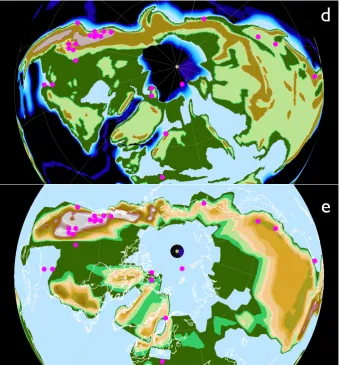
Table 1. Description of Proxy Data Sources and Treatment.
Locality 55 mya Mean upper lower CMM cmm Primary Reference Notes (adjusted) paleo- MAT error error error
latitude
Kisinger Lakes 47.5◦N 90.6◦W 22.90 3.60 3.60 6.70 Fricke and Wing (2004)
Chalk Bluffs 44.1◦N 102.7◦W 20.13 4.57 4.08 Hren et al. (2010) LMA data from Hren et al. (2010), recalculated with Kowalski and Dilcher calibration.
Chalk Bluffs 44.1◦N 102.7◦W 20.00 3.60 3.60 5.60 Fricke and Wing (2004) Values recomputed using Kowalski and Dilcher calibration
Green 45.6◦N 88.7◦W 24.50 7.20 7.70 7.30 1.5 Fricke and Wing (2004) Using Kowalski and Dilcher
River/Wind calibration
River
BHB Polecat 47.5◦N 88.4◦W 21.73 9.05 6.35 4.00 2.5 Wing et al. (2005)/ LMA-8 through LMA-4 from Wing
Bench Wing et al. (2000) et al. (2000). Values recalculated
with Kowalski and Dilcher calibration.
Kulthieth 57.8◦N 103.8◦W 19.40 1.00 1.00 12.60 Wolfe (2004) This is an old CLAMP number.
Camel’s Butte 49.5◦N 82.3◦W 17.8 3.60 3.60 3.50 Hickey (1977) This flora with very few specimens, which leads to anomalously low LMA temperatures, instead using the temperature derived in Hickey (1977), which is the preferred number used by later work, such as Wilf et al. (2000).
Yellowstone- 48.8◦N 90.8◦W 13.10 3.60 3.60 1.90 Fricke and Wing (2004) Values recalculated using Kowalski
Sepulcher and Dilcher calibration.
Republic 53.2◦N 98.4◦W 11.30 3.60 3.60 4.10 4 Greenwood et al. (2005) Percent entire margins from Greenwood et al. (2003) (used 8.8◦ from LMA 1) and used Kowalski and Dilcher calibration.
Princeton 54.6◦N 99.8◦W 5.00 3.60 3.60 5.30 2.8 Greenwood et al. (2005) Percent entire margins from Greenwood et al. (2003) and applied Kowalski and Dilcher calibration.
Quilchena 55.1◦N 99.8◦W 19.03 3.60 3.60 5.80 2 Greenwood et al. (2005) Percent entire margins from Greenwood et al. (2003) and applied Kowalski and Dilcher calibration. Age from 52 to 51 Mya.
Falkland 55.2◦N 98.5◦W 8.9 3.60 3.60 5.20 3 Smith et al. (2009) Percent entire margins from Greenwood et al. (2003) and applied Kowalski and Dilcher calibration gives 11.9 but using the later, better collection of Smith et al. (2009).
McAbee 55.5◦N 100.0◦W 12.80 3.60 3.60 3.50 4.4 Fricke and Wing As above. (2004)/Greenwood (2005)
Horsefly 57.5◦N 100.0◦W 12.86 3.60 3.60 5.30 2.8 Greenwood et al. (2005) As above.
Driftwood 60.6◦N 105.3◦W 8.25 3.60 3.60 2.70 5.6 Greenwood et al. (2005) As above. Canyon
Site 913 64.8◦N 5.2◦E 14.46 5.22 5.16 7.00 3 Eldrett et al. (2009) Longitude should be adjusted to 0 for site to be from Greenland. MAT values from 48 to 50 Ma. Error bars are maximum in time series (plus 1 stated error on that value) and the minimum of the time series (minus 1 stated error on that value).
Laguna del 46.9◦S 57.3◦W 20.72 5.76 6.63 10.80 3.8 Wilf et al. (2005) Location adjusted 3◦east. Based on
Hunco the analysis of Wilf et al. (2005),
Table 1. Continued.
Locality 55 mya Mean upper lower CMM cmm Primary Reference Notes (adjusted) paleo- MAT error error error
latitude
Brandy Creek 60.0◦S 148.7◦E 18.20 2.21 2.21 15.70 2.8 Greenwood et al. (2003, Position adjusted 2◦N and 3◦E.
2004) Percent entire margined from Greenwood et al. (2003, 2004), using Australian calibration.
Hotham 58.7◦S 149.9◦E 17.90 2.33 2.33 15.70 2.6 Greenwood et al. (2003, As above.
Heights 2004)
Dean’s 60.7◦S 145.7◦E 18.8 2.90 2.90 15.70 2.4 Greenwood et al. (2003, As described by Greenwood et al. Dean’s Marsh 2004) Marsh LMA is anomalously low and based
on personal communication with Greenwood the “bioclimatic method” MAT derived in those papers is preferred as the the macrofloral collection was poorly characterized and has been subsequently lost in a fire, whereas the bioclimatic estimate is robust and can be verified. Puryear- 37.1◦N 70.7◦W 35.30 3.60 3.60 16.10 Fricke and Wing (2004) Values recalculated using the
Buchanan Kowalski and Dilcher calibration. Paleolocation assumes location is near Puryear, TN.
Axel Heiberg 77.5◦N 35.3◦W 14.70 0.70 0.70 3.70 3.30 Greenwood et al. (2010) Values directly from Greenwood et al. (2010). These may be middle Eocene (Lutetian).
Axel Heiberg – 77.5◦N 35.3◦W 12.80 4.30 4.30 Greenwood et al. (2010) As above. US 188
Ellesmere 75.5◦N 28.0◦W 8.00 7.00 7.00 0.00 7.00 Eberle et al. (2010) Values directly from Eberle et al.
Island (2010), derived fromδ18O in biogenic phosphate. Early Eocene in age.
ACEX IODP 83.58◦N 27.23◦E 18.30 1.20 1.90 Weijers et al. (2007) No land in model near core 302 location, so using nearest land at
around 75◦N 64◦E. GPLATES
reconstruction at 55 Ma for the ACEX core is adjusted to paleo-shoreline which is further south than stated. Values taken from Weijers et al. (2007), using Core 29, early Eocene. No meaningful error bars stated in that paper.
Chuckanut, 53.6◦N 102.4◦W 15.50 0.50 0.50 11.50 1.50 Mustoe et al. (2007) CLAMP MAT from Mustoe et al.
WA (2007).
Harrell Core, 33.0◦N 71.7◦W 32.00 2.00 2.00 van Roij (2009) Location may be adjusted north
Meridian, MS to match land mask, error around
±2◦. Bashi/Hatchetigbee from van Roij Masters thesis. MBT/CBT temperature is approximate. Geiseltal, 46.9◦N 7.3◦E 23.95 1.05 1.05 19.00 2.00 Mosbrugger et al. (2005) Basal Lutetian age (as old as∼49
Germany Ma). MAT based on CA approach. Fushun, China 46.8◦N 122.2◦E 15.85 0.45 0.45 5.00 3.00 Wang et al. (2010) Values based on macrofloral data,
Table 4 of Wang et al. (2010). Mahenge, 18.3◦S 30.8◦E 36.50 3.60 3.60 Harrison et al. (2001) Location adjusted by 6◦E. Age is Tanzania ∼45 Ma, included for lack of other data.
Flora is probably not completely counted and this number is not likely to be robust,
but 17 out of 18 members of the flora were entire margined. Kowalski and Dilcher calibration used. Chermurnaut 68.0◦N 166.7◦E 18.20 3.96 3.97 Collinson and Hooker Based on Collinson and Hooker
Bay, Kamchatka (2003) summary, based on the work of
Budantsev (as cited in Akhmetiev) GPLATES 67.7◦N 171.0◦E.
Table 1. Continued.
Locality 55 mya Mean upper lower CMM cmm Primary Reference Notes (adjusted) paleo- MAT error error error
latitude
Fossil Hill 62.9◦S 62.3◦W 16.74 3.60 3.60 7.60 Li (1992) Percent entire margins is from
Flora, King Li (1992). Calculated with Kowalski George Island, and Dilcher calibration. Age is Antarctica considered 49–42 Ma but is subject
to varying considerations. James Ross 64.9◦S 61.1◦W 16.10 4.00 4.00 7.60 Poole et al. (2005) JRB averages from Poole et al.
Basin, (2005) using co-existence approach. Antarctica Values from Table 3. Age is listed
as early Eocene.
Dragon 62.8◦S 61.7◦W 12.90 3.60 3.60 10.00 0.80 Hunt and Poole (2003) Values recalculated with Kowalski Glacier, King and Dilcher calibration. George Island,
Antarctica
China Gulch 43.3◦N 103.38◦W 24.51 1.50 1.50 Hren et al. (2010) 5.3◦C km−1lapse rate correction applied to MBT/CBT numbers of Hren et al. (2010), with 1.5 “reproducibility” errors. Camanche 43.3◦N 103.4◦W 25.98 1.50 1.50 Hren et al. (2010) As above.
Bridge
Pentz 44.8◦N 103.8◦W 24.00 1.50 1.50 Hren et al. (2010) As above.
Cherokee Site 1 44.8◦N 103.8◦W 16.59 1.50 1.50 Hren et al. (2010) As above. Fiona Hill 44.1◦N 103.1◦W 16.70 1.50 1.50 Hren et al. (2010) As above.
Council Hill 44.7◦N 103.2◦W 21.63 1.50 1.50 Hren et al. (2010) As above. Iowa Hill 44.2◦N 103.2◦W 22.96 1.50 1.50 Hren et al. (2010) As above. You Bet 2 44.3◦N 103.1◦W 23.80 1.50 1.50 Hren et al. (2010) As above.
Chalk Bluffs – 44.3◦N 103.2◦W 26.75 1.50 1.50 Hren et al. (2010) As above. E
Scotts Flat 44.4◦N 103.2◦W 24.91 1.50 1.50 Hren et al. (2010) As above.
Gold Bug 44.5◦N 103.2◦W 25.08 1.50 1.50 Hren et al. (2010) As above. Hidden Gold 44.2◦N 103.2◦W 18.38 1.50 1.50 Hren et al. (2010) As above.
Camp
Woolsey Flat 44.5◦N 103.1◦W 24.84 1.50 1.50 Hren et al. (2010) As above. Mountain Boy 44.7◦N 103.2◦W 19.84 1.50 1.50 Hren et al. (2010) As above. Pine Grove 1 44.8◦N 103.1◦W 22.82 1.50 1.50 Hren et al. (2010) As above.
Otaio 56.1◦S 163.7◦W 15.97 2.99 2.99 11.00 3.76 Hollis et al. (2011) Early Eocene of New Zealand, using Australian LMA calibration. Provided by Liz Kennedy.
The published error bars around winter season temperature reconstructions are non-negligible and those around summer temperatures are even larger. More concerning are the con-ceptual issues involved in using modern floral/climate re-lationships to estimate past climate regimes with no clear analogue (Utescher et al., 2009), such as subtropical cli-mates in polar night. When strongly restrictive and con-served biophysical-derived traits are involved, such as is clearly the case with freezing temperatures and palm trees and crocodiles, the proxy data provide a stronger constraint than in regions of climate regime space where no clear strong biological constraints exist or which no flora currently oc-cupy. Our approach is that constraints on summer terrestrial
implicitly can only explore climate parameter spaces experi-enced by modern vegetation are likely to be of limited value. Because of a lack of modern analogue in climate-ecosystem space for these hot,wet conditions, a strong asymmetry ex-ists between the ability to constrain increases in CMM and increases in warm month mean (WMM), except perhaps at high latitudes where WMM conditions may lie within the modern climate envelop (of low latitude conditions). On the other hand, light limitation, in the form of short, but 24-hour growing seasons almost certainly introduces a layer of complexity in interpreting growing season, and hence WMM temperatures at high latitudes.
Based on these considerations, we focus attention on the winter season aspect of the equable climate problem and do not make a quantitative comparison with summer tempera-ture proxy reconstructions. In this study, we find that win-ter temperatures were above freezing everywhere except for interior Antarctic and small regions of high paleoelevation, primarily restricted to western North America. We adopt a two-pronged approach to model-data comparison for winter temperatures.
First, we show that seasonal-mean modelled temperatures everywhere (with the exceptions mentioned) were above freezing. This broad-strokes approach enables comparison with many of the crucial but qualitative indicators and char-acterizations of warm winters that are ubiquitous in the early Eocene geological record, including inferences from floral and faunal assemblages and soil and clay types, (Greenwood and Wing, 1995; Markwick, 2007; Pigg and Devore, 2010; Collinson and Hooker, 2003; Valdes, 2000). Such indica-tors provide important constraints but are difficult to directly compare quantitatively with model output (although see Sell-wood and Valdes, 2006 for one excellent approach).
The second approach we employ is to compare CMM tem-peratures predicted by the models, point by point, with those inferred from paleoclimate proxies. This approach is quan-titative and provides explicit error bars, but estimates may not be altogether accurate for all the reasons described pre-viously for MAT. Furthermore, when considering the error bars on CMM estimates, it is important to consider that lower bounds on CMM are more likely to be accurate because those involve strong biological/physical constraints (i.e. palms do not tolerate freezing). The upper error bound on CMM is probably less constrained. Such CMM estimates are not as broadly available as the qualitative records but are as roughly comparable in their extent as the MAT records and often derive from the same analyses. In this study we compile CMM estimates primarily derived from CLAMP but supple-mented by other sources, such as isotopic analysis and the co-existence approach. The error estimates are derived from the primary sources and do not account for temporal varia-tion, unlike the MAT error bars. The CMM estimate sources are detailed in Table 1.
3.1.3 Uncertainties in topography, timing, and paleolocation
A major source of ambiguity in model-data comparison is the difference between the modelled elevation and the ac-tual elevation of the proxy locality. Errors of ∼6◦C can be introduced by a 1 km difference in elevation between model and data (Sewall et al., 2000). Every effort has been made to minimize this error by making the most accurate reconstruction of paleoelevation utilizing the available in-formation at the time (Sewall et al., 2000). But, such esti-mates are controversial and have uncertainty associated with them of at least±500 meters in mountainous regions where much of the proxy data are found (Peppe et al., 2010; Hren et al., 2010; Rowley, 2007; Forest, 2007; Meyer, 2007; Mol-nar, 2010). Paleoelevation scholarship has progressed in the decade since our topography dataset was created and many important details have changed. Nevertheless, little consen-sus exists on those details (Davis et al., 2009; Mulch et al., 2007; Molnar, 2010) so it is difficult to meaningfully improve the situation at the moment.
Even if the mean elevation of a region was correctly repre-sented by the elevation of a given model grid cell, error can be introduced by the fact that many proxy records are found within basins in high relief regions. This bias in preservation can introduce large errors even when the gross features of to-pography are fully correct in the model (Sewall et al., 2000). Thus the real errors are probably closer to±1000 m in high elevation, high relief regions such as intermontane western North America.
We quantify that uncertainty here by calculating the stan-dard deviation of topography averaged over all elevations greater than 1500 m in a modern high-resolution digital el-evation model. Utilizing the average 2-σ topographic vari-ation in modern topography (450 m) as an estimate of relief in regions of high mean elevation in the Eocene, we find a ±2.4◦C uncertainty in temperature introduced as a result of relief, assuming a 5.3◦C km−1lapse rate based on the work of Hren et al. (2010).
Temporal sampling uncertainty is also a concern since a modelled time slice represents millions of years, whereas substantial evidence exists for climate fluctuations of±5◦C at a single location over that time scale (Wilf et al., 1998; Wilf, 2000; Bao et al., 1999; Wing et al., 2000, 2005). Con-sequently, wherever a time series is available at a locality, we compare the mean as well as the maximum and minimum of the series with the stated random calibration error of the indi-vidual proxy data points superimposed. Where a single data point is available, we utilize the stated methodological error although these certainly underestimate the true error range.
the model grid (i.e. differences in reference frame). This is exacerbated by uncertainty in true paleotopography and sea level and the differences between these and the mod-elled representation of these real-world features. The uncer-tainty in temperature assignable purely to unceruncer-tainty in a locality’s true paleolatitude and longitude is relatively small (<2◦C), both because the position errors themselves are rather small (∼ ±2◦ latitude, ±5◦ longitude) and because early Eocene temperature gradients were quite small (Green-wood and Wing, 1995). More important is the fact that there can be large differences in absolute paleoposition between two reconstructions, and specifically between the reconstruc-tion that was the basis for the model grid (Sewall et al., 2000) and more recent reconstructions (Markwick, 2007; Mueller et al., 2008).
If, for example, recent reconstructions indicate that North America was 5◦further south than the reconstruction in the
model, should the model-data comparison be performed at the true paleolatitude and longitude, or at the appropriate model grid paleolatitude and longitude? Or should the tem-perature estimate from the model grid be corrected back to its correct latitude using an empirical correction? Provided temperature gradients are weak, this is not a large source of uncertainty, introducing perhaps 2.5◦C error in the example given, but it has the potential to be a systematic bias.
This can be a more substantial problem in an occasional situation, such as the MBT-CBT record of Weijers et al. (2007a) or the palynological record of Eldrett et al. (2009) which are derived from marine cores and the location of ter-restrial source region is primarily conjectural and reflects ei-ther a localized source or an integrated signal from regions that are not tightly constrained. As shown below, the poten-tial error associated with this is not estimated to be large.
Further ambiguity and room for error arises when there is a large mismatch between the classification of a locality as land or ocean between the model and reality. For example, near the Gulf Coast of North America or in New Zealand, the true paleolocation of a terrestrial site places it solidly in the ocean on the coarse-resolution model grid. This intro-duces the problem of deciding to use the nearest available terrestrial grid cell or the nearest grid cell for comparison re-gardless of whether it is land or ocean. In the case of New Zealand, the South Island was small and barely sub-areal, so it is simple to consider the nearest ocean grid cell as being a reasonable estimator to the terrestrial temperature, but with difficult to quantify error associated with the approximation. For the Gulf Coast data a better approach, given the weak temperature gradients, is to use the nearest land surface grid cell which is more likely to properly account for land-sea temperature contrasts.
It is for these reasons that it is common in model-data com-parison studies to compare zonal mean model-derived tem-peratures with proxy data (Huber and Sloan, 2001; Shellito et al., 2003). It is hoped that many of these errors will can-cel out when the data are aggregated and averaged. Whether
or not comparing sparsely-sampled data with zonal means actually leads to a robust characterization of model-data dif-ference has never been quantitatively answered. Pointwise comparison of models and data has been shown to be im-portant in establishing model fidelity in reproducing climate trends in the recent observational record (Duffy et al., 2001) and it seems likely to be a better approach, albeit more chal-lenging, because it requires accounting for random errors and bias in geographic assignment.
3.2 Modelling
As described in previous work, Eocene conditions have been simulated with a fully-coupled general circulation model, the National Center for Atmospheric Research (NCAR) Community Climate System Model version 3 (CCSM3). These simulations span a range ofpCO2from 560 ppm to 4480 ppm. After synchronous, coupled integration of 2000– 5000 years (some simulations equilibrate faster than others), all the simulations equilibrated in terms of surface and global mean ocean temperature and ocean “ideal age” tracers. As-pects of the coupled simulations with a focus on the ocean circulation are described in Liu et al. (2009) and Ali and Hu-ber (2010). The ocean-atmosphere circulation of these simu-lations are similar to those of Winguth et al. (2010) and Shel-lito et al. (2009), who utilized the same model with nearly identical boundary conditions, although the simulations were not integrated as long and the solar constant and aerosol treat-ments were somewhat different. Winguth et al. (2010) pro-vide a good overview of the ocean-atmospheric dynamics simulated by CCSM3 for Eocene conditions that are repre-sentative of those in the simulations described here.
The mixed layer depth, sea surface temperature (SST), sea ice fraction, and ocean heat convergence patterns de-rived from these coupled simulations were utilized to create mixed-layer “slab” oceans for coupling to the atmospheric component of CCSM3, the CAM3. Interesting aspects of the atmospheric dynamics produced in the simulations were described elsewhere (Caballero and Huber, 2010; Williams et al., 2009; Sherwood and Huber, 2010; Eldrett et al., 2009). Of specific importance to this study, an important high lati-tude feedback in CAM3 was shown to enhance warming near the poles in the Eocene (Abbot et al., 2009b).
1365 W m−2, aerosol radiative effects were set to zero, and other trace gas concentrations and orbital parameters were set to pre-industrial conditions. The land surface boundary conditions used were the same as described in Sewall et al. (2000) although they have been reinterpolated from the orig-inal 2◦×2◦data to T42 resolution as opposed to the T31 res-olution version that was used in much of the previously de-scribed work (Huber and Sloan, 2001; Huber and Caballero, 2003; Shellito et al., 2003, 2009; Winguth et al., 2010). Shorter simulations at resolutions up to T170 (0.7◦×0.7◦) were carried out and the results discussed here are robust at higher resolution.
Here we present results of simulations from the NCAR CAM3.1 at T42 resolution driven by these speci-fied SSTs derived from coupled simulations. The fixed SST simulations were carried out for>50 years to ensure equi-librated climatologies and means were calculated over the last 25 years. The main simulation, referred to as EOCENE-4480, was carried out with 4480 ppmv CO2and is meant to represent the early Eocene. As described previously, this does not imply that 4480 ppmv is the actual value for the early Eocene; it is merely the radiative forcing necessary for a climate model with a weak sensitivity to achieve climate conditions close to those of the early Eocene. For context and to give an indication of the robustness of these results we, have included results from another case, EOCENE-2240, carried out with 2240 ppm CO2 and which we have previ-ously shown is a better fit to mid-to-late Eocene climate (El-drett et al., 2009).
In Sect. 4 we present a comparison of zonal mean model results for modern and Eocene conditions, maps of mod-elled Eocene surface temperatures, and pointwise compari-son of proxy data and model results. For this comparicompari-son, all proxy records were rotated back to their paleo-locations at approximately 55 mya utilizing the GPLATES software (www.gplates.org) and plate model of Mueller et al. (2008) with some slight adjustments made to accomodate georefer-encing differences between the model plate locations and the GPLATES reconstruction.
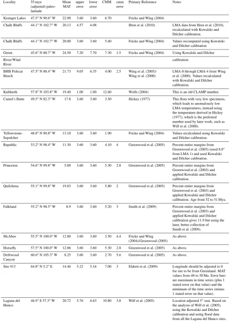
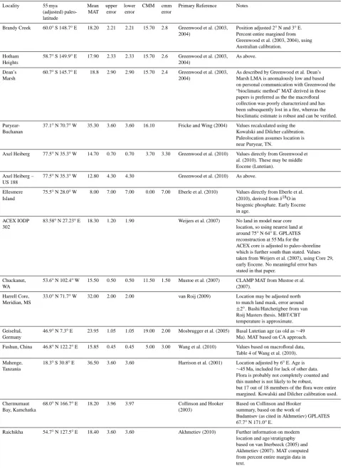
First, the modern location of the paleo-localities was in-troduced into GPLATES and then the localities were rotated back to their positions at 55 mya (Fig. 1a). The plate lo-cations determined by GPLATES (http://www.gplates.org) were then compared with the paleogeography utilized in the modelling, derived originally from Sewall et al. (2000) in order to determine that they were generally compara-ble (Fig. 1b−c, 1d−e). In almost all cases, the paleo-geography in the model was consistent with the GPLATES 55 mya reconstruction and where adjustments were neces-sary, they were objectively determined by comparing con-tinental boundaries and making uniform, small adjustments to GPLATES reconstructed latitude and longitude to align correctly with geographic features in the model paleogeogra-phy. When this was done, model predictions were compared with proxies at these adjusted locations and inspection of the
results was used to evaluate that the potential errors intro-duced by differences in true and modelled paleo-location are small (Fig. 1d−e).
Furthermore, a comparison of the model paleogeography we used and the early Eocene paleotopography indepen-dently derived by Paul Markwick (Markwick, 2007) revealed that our reconstructions were in general agreement, indicat-ing robustness of general features but differindicat-ing in important details, for example in intermontane western North America (Fig. 1d−e, 1f). In the subsequent model-data comparison, we accounted for uncertainty in the true paleolocation, its temporal variation over the early Eocene, and the discretiza-tion introduced by the model grid by including error bars of ±2.5◦ latitude on both proxy records and the model re-sults. A spreadsheet including the references and values used in the paleotemperature reconstruction has been included as supplemental material. The GPLATES Markup Language (GPML) file used to rotate modern localities is also available as supplemental material.
4 Results
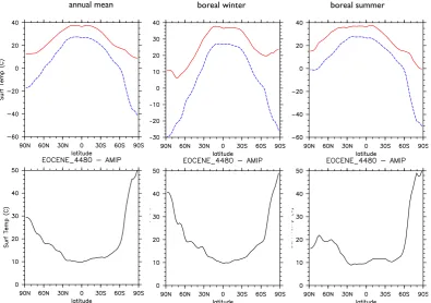
4.1 Modeled zonal-mean surface temperatures
As an overview of the climate changes occurring in the Eocene simulation, Fig. 2 compares modeled zonal-mean surface temperatures from the EOCENE-4480 run with a CAM3 simulation using modern boundary conditions as specified by the Atmopheric Model Intercomparison Project (AMIP). In AMIP simulations, modern, observed SSTs (and other boundary conditions) are specified. The zonal mean includes averaging over both land and ocean. At high lati-tudes, the Eocene case is 30–50◦C warmer than modern in both MAT and seasonal means. Differences are more muted in the tropics,ranging from 6–10◦C in all seasons. These results qualitatively capture the salient features noted in the proxy temperature record (Barron, 1987): annual mean tem-peratures much warmer than modern, especially at high lat-itudes, winter season temperatures generally above freezing, and a much reduced equator-to-pole temperature gradient. The hemispheric asymmetry in temperature increase is con-sistent with the removal of the Antarctic Ice Sheet and the associated 15–20◦C change associated with the decrease in elevation.
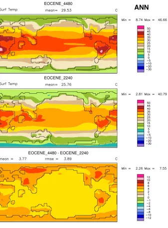
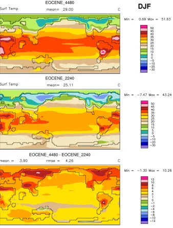
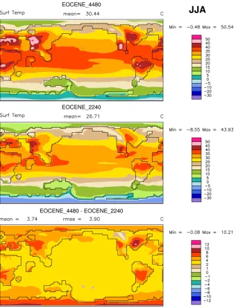
4.2 Maps of modeled surface temperatures
a
Fig. 1a. Comparison of paleogeographic information used in the simulation with independent reconstructions from Mueller et al. (2008) via the freely available GPLATES software and via personal communication from Paul Markwick. In (a) a plate tectonic reconstruction for 55 mya from GPLATES including sea floor age is shown. Terrestrial paleoclimate proxy localities are indicated on this map with green circles. The modern continental boundaries in their 55 mya positions as reconstructed by GPLATES compard with Markwick’s paleogegraphy are shown in (b, d). The topography used in model (c, e) is compared with the independently derived high resolution early Eocene topography of Markwick (based on Markwick (1998)) (b, d). In these figures, the paleoclimate proxy localities are indicated with magenta circles. The GPLATES derived plate configuration is a reasonable match to the land-sea distribution developed in Sewall et al. (2000) used in the simulations here (c, e). It should be noted that in some cases GPLATES derived paleolocations must be adjusted slightly to fall on land or to be in the right location with respect to topography, as described in the text. In (f) an example of how the pointwise comparison of model and proxy records is performed is shown. Colors are modelled temperatures and the text indicates the abbreviated names of proxy localities. Based on modern latitude and longitudes the localities are rotated back to 55 mya positions using GPLATES, thus enabling the best objective placement of the paleo-positions within the model’s reference frame. As (f) shows, errors in paleo-position are unlikely to introduce large errors in inferred temperature except in regions with strong temperature gradients, i.e. in regions of strong elevation variation.
SSTs are about 35◦C, in general agreement with proxies (Pearson et al., 2007; Huber, 2008; Jaramillo et al., 2010; Schouten et al., 2007). The hottest temperatures are on land in the subtropics, where annual mean values are 45◦C. No proxy records currently exist to support or refute this result.
Winter temperatures in the EOCENE-4480 case remain above freezing everywhere except for inland Antarctica. Temperatures in intermontane western North America dip near zero in agreement with the existence of microthermic flora – though with an absence of frost intolerant macroflora – in various upland localities in the region (Smith et al., 2009). Maximum terrestrial temperatures in summer of up to 50◦C are reached in northern and southwestern Africa, southern central South America, southwest North America, central Europe and western central Asia. The interiors of North America and Amazonia are also very hot (>40◦C) in summer. It should be noted that these are seasonal (3-month) means and that temperature extrema on subseasonal
time scales may be substantially higher; we present seasonal means here since they are likely to best reflect the processes that shape the long-term distribution of proxies, flora and fauna. A comparison with the coldest climatological monthly mean temperature is carried out below for strict comparison with CMM proxy records.
b
c
Fig. 1b−c. Figure 1 continued, see Fig. 1a for description.
Localized warming is also evident in austral winter in the interior of Antarctica and in the boreal summer of west cen-tral Asia, and in midlatitude North America and Europe. These results show that localized temperature changes of up to 10◦C can occur seasonally even with globally homoge-neous forcing and annual-mean SST change of less than 3◦C everywhere. Though the EOCENE-2240 case is very warm and has no sea ice, the additional greenhouse gas forcing in the EOCENE-4480 case yields a polar-amplified warm-ing, with most of the amplification occurring in the winter season. The overall pattern is quite similar to the effect of doublingpCO2in modern CAM3/CCSM3 simulations, de-spite the large differences in continental configuration, back-ground greenhouse gas values, and other boundary condi-tions. Polar ampliflication in the absence of sea-ice has been attributed in various studies to increased latent heat transport (Langen and Alexeev, 2007; Caballero and Langen, 2005) and to high-latitude cloud feedbacks (Abbot et al., 2009a,b); the latter have been shown be especially important in Eocene
CAM3 simulations. Much of the terrestrial winter response seen here (between the two Eocene cases) correlates well with the near complete loss of snow cover and associated albedo decreases in the EOCENE-4480 case.
d
e
Fig. 1d−e. Figure 1 continued, see Fig. 1a for description.
f
annual mean boreal winter boreal summer
Fig. 2. Zonal mean surface temperature from the EOCENE-4480 (red) and modern, AMIP (blue) simulations as described in the text. In the upper row, the annual (left) boreal winter (middle) and boreal summer (right) means are shown. In the lower row, the anomaly, EOCENE-4480 minus modern, AMIP simulation is shown.
4.3 Pointwise data-model comparison
Pointwise comparison of proxy data and EOCENE-4480 modeled MAT (Fig. 4) reveals reasonably good overall agreement. Substantial scatter in the proxy data is apparent in the Northern Hemisphere midlatitudes, but is due mostly to data from intermontane western North America and likely reflects real gradients in topography and surface temperature that are not well represented in the low resolution topography used in the model (Fig. 5). The model and data generally agree within their respective errors, which include a gross estimate of uncertainty due to modelled versus real elevation in mountainous regions, as discussed in Sect. 3.1.3. Both simulated and proxy data MATs are∼35◦C at the poleward edge of the subtropics. The model does not appear to cap-ture the peak high latitude temperacap-tures derived from MBT-CBT, although it does capture warm temperatures on Axel Heiberg and Ellesmere Islands. The Axel Heiberg Island proxy records may reflect cooler conditions because they are middle Eocene in age, but the Ellesmere Island data, which is early Eocene in age produces a similar MAT, so the fact that the model matches the data at these high latitude sites is not necessarily attributable to temporal sampling issues. It has been conjectured that the MBT-CBT proxy may be biased to summer values (Weijers et al., 2007a; Eberle et al., 2010), in which case the data and model are more concordant.
Inspection of Fig. 4b suggests that the model does not suf-fer from a strong bias either to hot or cold temperatures, with roughly equal numbers of points falling on either side of the 1:1 line.The mean data-model difference is 0.7◦C, while the standard error is 1.3◦(assuming all data points are uncorre-lated), implying that there is no statistically significant over-all bias. This lack of global bias is qualitatively confirmed on a regional basis by Fig. 5, which shows positive and negative errors scattered randomly with no obvious bias in any region. On the other hand, the 2 largest model-data discrepancies are both on the warm side, with the model overestimating the data by roughly 9◦C. Most of the errors lie in regions of
steep orography (Figs. 1d−e, 5), with a slight tendency for overprediction of temperatures by the model at lower eleva-tion and underprediceleva-tion of temperatures along topographic highs; these discrepancies plausibly result from errors in pa-leolocation of paleoelevation. These nearly bias-free results are a vast improvement over our previous model-data com-parison (Huber et al., 2003), which used an older version of the NCAR coupled model with 560 ppmv CO2and showed model MATs systematically offset from proxy data by 10◦C or more over large parts of the globe.
M. Huber and R. Caballero: Eocene equable climates revisited 619
Fig. 3a.Maps of time averaged surface temperature from the EOCENE-4480 and EOCENE-2240 simulations. The annual (a), boreal winter (b), and boreal summer (c) means are shown. The upper row is the EOCENE-4480 case, the middle row is the EOCENE-2240 case, and the bottom row is the anomaly. The range is values is indicated in the color bar in (a) and is the same in (a-c). Units are in◦C
Fig. 3a. Maps of time averaged surface temperature from the EOCENE-4480 and EOCENE-2240 simulations. The annual (a), boreal winter (b), and boreal summer (c) means are shown. The upper row is the EOCENE-4480 case, the middle row is the EOCENE-2240 case, and the bottom row is the anomaly. The range is values is indicated in the color bar in (a) and is the same in (a–c). Units are in◦C.
climatology to be as close to possible to the standard definition of CMM employed in paleoclimate reconstruc-tions. Correspondence is excellent, even in mid-to-high lat-itude regions that have previously been challenging (Shel-lito et al., 2003). The main remaining discrepancy is at the Puryear-Buchanan site (37.1◦N, 70.7◦W, see table), where the model produces a CMM of nearly∼25◦C whereas the
data are∼16◦C. This may not be too serious given that there
is wide uncertainty in the proxy data estimate (Greenwood and Wing, 1995) and other nearby localities, albeit from marine proxies, show winter temperatures of 21.6–24.3◦C
(Kobashi et al., 2004). The model is clearly capable of matching both the general qualitative pattern of a frost-free early Eocene (Fig. 3b), while giving a good quantitative match to winter temperature minima where such data exist (Fig. 6).
Fig. 3b. Figure 3 continued, see Fig. 3a for description.
Abbot et al., 2009b). To establish the point-by-point degree of temperature change, we take the anomaly of proxy-based Eocene MAT estimates compared to modern observed MAT at the same location. Modern MAT from the European Cen-ter for Medium-Range Weather Forecasts 40-Year Reanaly-sis Project (ERA-40) was used for modern observations. To calculate the pointwise warming of the model with respect to modern, we compare the MAT anomaly point-by-point be-tween the EOCENE-4480 case and the modern CAM3 AMIP simulation discussed in Sect. 4.1. This comparison (Fig. 7) reveals a generally very good correspondence between the modelled and reconstructed warming at all latitudes. The zonal-mean modelled temperature anomaly with respect to
modern conditions gives a good overall agreement with the observational anomalies, though regional and local details in-troduce significant scatter. Overall, it appears that the model is capable of quantitatively reproducing the polar amplifica-tion of terrestrial warming in passing from modern to early Eocene conditions.
5 Discussion
Fig. 3c. Figure 3 continued, see Fig. 3a for description.
were much warmer than previously reconstructed (Covey et al., 1996). Thus, revisiting the equable climate problem requires rethinking how to frame the problem. Most cli-mate model simulations have not investigated temperatures – including tropical temperatures – nor greenhouse gas forc-ing, in the ranges now considered likely. Our perspective in this paper is that most previous attempts to solve the equable climate problem have suffered from the question being ill-posed. Climate was even warmer than previously reconstructed and the forcing or climate sensitivity were also probably larger. Utilizing these new higher temperature ter-restrial reconstructions for comparison makes the model-data comparison more challenging than some prior attempts given
0 5 10 15 20 25 30 35 40
-90 -60 -30 0 30 60 90
MAT °C
Latitude
0 5 10 15 20 25 30 35 40
0 5 10 15 20 25 30 35 40
M
od
el
le
d
M
A
T
°
C
Proxy MAT °C 0
5 10 15 20 25 30 35 40
-90 -60 -30 0 30 60 90
MAT °C
Latitude
Fig. 4. On the left, a pointwise comparison of annual mean terrestrial surface temperature (MAT) from EOCENE-4480 (red) and proxy data estimates (green) versus latitude. The vertical error bars on the proxies represent the methodological error plus the temporal variation (if a time series) as further described in the text. The model vertical error bars are only included in regions considered to have high elevation and represent topographic uncertainty as described in the text. Horizontal error bars indicate the uncertainty in the position of the paleolocality and the propagation of that uncertainty onto the discrete model grid (as described in the text). A comparison is also made for reference of tropical SSTs (reconstructed in blue and modelled in magenta). The tropical reconstructions follow those in Huber (2008) with the exception of the Tanzanian (19 South latitude) TEX86data which were recalculated using the Liu et al. (2009) calibration. It should be noted that the potential uncertainty is underestimated, since only one set of calibrations was used for each proxy and therefore a major source of uncertainty is ignored. On the right, the temperatures reconstructed from terrestrial proxies are plotted versus modelled and the 1-to-1 line is plotted in black. The error bars are the same as previously described.
5
Fig. 5. Difference between modelled and reconstructed MAT as indicated by the color bar(on the right) overlain on the the model predicted temperatures (grey scale color bar on left).
Model-data discrepancies remain, however. These do not appear to be of a magnitude that a compelling case for com-pletely “missing physics” can be made, but they do point to many areas that need improvement. But, as described pre-viously in Sects. 2 and 3.1.3 there may be limits to how well we can ever expect the simulations to match observa-tions, given the incompleteness of the record and, of course,