https://doi.org/10.5194/amt-10-3117-2017 © Author(s) 2017. This work is distributed under the Creative Commons Attribution 3.0 License.
Estimating trends in atmospheric water vapor and
temperature time series over Germany
Fadwa Alshawaf1, Kyriakos Balidakis2, Galina Dick1, Stefan Heise1, and Jens Wickert1,2 1German Research Centre for Geosciences GFZ, Telegrafenberg, 14473 Potsdam, Germany 2Institute of Geodesy and Geoinformation Science, Technische Universität Berlin,
Straße des 17. Juni 135, 10623 Berlin, Germany
Correspondence to:Fadwa Alshawaf (fadwa.alshawaf@gfz-potsdam.de) Received: 13 March 2017 – Discussion started: 23 March 2017
Revised: 1 August 2017 – Accepted: 2 August 2017 – Published: 31 August 2017
Abstract. Ground-based GNSS (Global Navigation Satel-lite System) has efficiently been used since the 1990s as a meteorological observing system. Recently scientists have used GNSS time series of precipitable water vapor (PWV) for climate research. In this work, we compare the tempo-ral trends estimated from GNSS time series with those es-timated from European Center for Medium-Range Weather Forecasts (ECMWF) reanalysis (ERA-Interim) data and me-teorological measurements. We aim to evaluate climate evo-lution in Germany by monitoring different atmospheric vari-ables such as temperature and PWV. PWV time series were obtained by three methods: (1) estimated from ground-based GNSS observations using the method of precise point po-sitioning, (2) inferred from ERA-Interim reanalysis data, and (3) determined based on daily in situ measurements of temperature and relative humidity. The other relevant atmo-spheric parameters are available from surface measurements of meteorological stations or derived from ERA-Interim. The trends are estimated using two methods: the first applies least squares to deseasonalized time series and the second uses the Theil–Sen estimator. The trends estimated at 113 GNSS sites, with 10 to 19 years temporal coverage, vary between −1.5 and 2.3 mm decade−1 with standard deviations below 0.25 mm decade−1. These results were validated by estimat-ing the trends from ERA-Interim data over the same time windows, which show similar values. These values of the trend depend on the length and the variations of the time series. Therefore, to give a mean value of the PWV trend over Germany, we estimated the trends using ERA-Interim spanning from 1991 to 2016 (26 years) at 227 synoptic sta-tions over Germany. The ERA-Interim data show positive
PWV trends of 0.33±0.06 mm decade−1 with standard er-rors below 0.03 mm decade−1. The increment in PWV varies between 4.5 and 6.5 % per degree Celsius rise in temperature, which is comparable to the theoretical rate of the Clausius– Clapeyron equation.
1 Introduction
GNSS-based estimates of zenith total delay (ZTD) or PWV have been assimilated into numerical weather prediction models to improve the quality of the output (Bock et al., 2005; Bennitt and Jupp, 2012). They have also been used to im-prove the performance of high-resolution atmospheric mod-els (Pichelli et al., 2010). Besides meteorology, GNSS es-timates of PWV have been employed over Scandinavia for climatological research (Elgered and Jarlemark, 1998; Grad-inarsky et al., 2002; Nilsson and Elgered, 2008). The authors found that PWV shows an increase of 1.2–2.4 mm decade−1. Haas et al. (2003) used ground-based GPS, very long base-line interferometry, radiosonde, and microwave radiometer data to assess long-term trends in PWV time series over Swe-den. An increase of about 0.17 mm year−1within the period 1980–2002 was observed. Hausmann et al. (2017) analyzed a decadal time series of PWV (2005–2015) from mid-infrared Fourier transform infrared measurements above the moun-tain Zugspitze. For that time period, they did not observe statistically significant trend in PWV time series. The PWV time series from ground-based GNSS and the European Cen-ter for Medium-Range Weather Forecasts (ECMWF) reanal-ysis (ERA-Interim) data might show temporal inconsisten-cies due to, for example, hardware replacement or inconsis-tent processing methods (Ning et al., 2016). Therefore, ho-mogenization of the atmospheric data is indispensable for climatological research to properly estimate climatic long-term trends. Vey et al. (2009) and Ning et al. (2016) analyzed PWV time series estimated at global GNSS sites to detect and correct for inhomogeneities in the data. Atmospheric reanal-ysis models such as ERA-Interim have also been employed for climate research. The analysis fields are produced based on 4D-Var assimilation of regular and irregular meteorolog-ical data, including surface and upper-air atmospheric fields (Dee et al., 2011).
Bengtsson et al. (2004) observed an increasing long-term trend with a slope of 0.16 mm decade−1in the water vapor data set of ERA 40 within the period of 1958–2001. They suggested applying corrections for the changes in the ob-serving system when using the data for PWV analysis to achieve trend values comparable to GNSS. ERA-Interim and MERRA (Modern Era Retrospective-Analysis for Research and Applications) were also used for trend analysis (Sim-mons et al., 2007; Rienecker et al., 2008).
Typically, climate scientists consider a period of 30 years as an appropriate time necessary to average variations in weather and evaluate climatic effects for a particular site, as described by the World Meteorological Organization (Arguez and Vose, 2011). Data collected and averaged or summed in some way over 30 years are referred to as cli-mate normals. A 30-year period is recommended, as it is sufficiently long to filter out the interannual variations or anomalies but at the same time short enough to show climatic trends. It is then obvious that the GNSS temporal span is still too short for estimating a reasonably proper climatic trends in this sense. The previous studies using GNSS-based PWV
time series for assessing the trends show highly variable esti-mates for different time windows as well as different research regions. In this paper, we present the PWV trends estimated using GNSS sites over Germany and compare them with the trends estimated from other data sets. The current climate normal period should cover the period from 1 January 1991 to 31 December 2020 (Arguez and Vose, 2011). So, we ana-lyzed time series available from 1 January 1991 to June 2016 (26 years) to provide more robust information about the cli-matic trends. These data sets are the ERA-Interim reanalysis and surface meteorological data from the German Meteoro-logical Service (DWD). The former data set provides global PWV grids while the latter does not. However, different stud-ies have used the dew point that is computed using surface measurements of temperature and relative humidity to ap-proximate the total column PWV (Reitan, 1963; Bolsenga, 1965; Smith, 1966; Tuller, 1977). The formula presented to obtain the PWV from surface measurements is described in Sect. 4. This empirical relation requires only information that can accurately be determined on the ground. The accuracy of dew-point-based PWV approximations depends of course on the atmospheric conditions and the variability of the mois-ture profiles. It is, however, obvious that PWV estimations based just on atmospheric conditions at the Earth’s surface would not always be in complete agreement with, for exam-ple, PWV values from balloon soundings integrated through the atmosphere. Since the possibility for obtaining a data set with long time series and high spatial resolution for estimat-ing PWV trends is very limited, we evaluated the potential of this method for climate analysis. We first obtained the PWV based on dew point temperature measurements and evaluated the quality of the time series. Then we used them to esti-mate the PWV as well as temperature trends. In this work, we apply a preprocessing step to evaluate the quality and ho-mogeneity of the time series ahead of the trend estimation. For checking the homogeneity of the time series, we use the ERA-Interim as a reference. We apply the technique of sin-gular spectrum analysis to detect possible change points fol-lowed by attest to identify the significance thereof. The de-scription of the approach for homogeneity check is beyond the scope of this paper and details are found in Wang (2008) and Ning et al. (2016).
it is still below the normal (30 years), suggested by climatol-ogists, we extended the research using other data sets (e.g., ERA-Interim and synoptic data). First, it is more reasonable to give a mean value of the change per decade (trend) us-ing longer time series; second, usus-ing time series of the same length at all sites in the research region enables us to observe specific spatial features of the trend, as presented later in the paper. We also calculate the change in PWV per degree Cel-sius rise in temperature to check if it is consistent with the Clausius–Clapeyron relation.
This paper is organized as follows. In Sect. 2, we describe the method for PWV determination using GNSS data and the comparison with ERA-Interim. In Sect. 3, we present the methods for estimating the atmospheric trends followed by the results of estimating the decadal rate of change in Sect. 4. Then, the conclusions of this research are presented.
2 Determination of atmospheric PWV from GNSS data We used GPS data collected in central Europe, mainly in Ger-many as shown in Fig. 1. The research region is well cov-ered by 351 permanent GNSS sites with an average separa-tion distance of 30 km. Homogeneous time series with length from 10 to 19 years are available from 119 sites. The second data set we used is the ERA-Interim reanalysis with a spa-tial resolution of 79 km in longitude and latitude, 60 verti-cal levels with the model top at 0.1 hPa (about 64 km), and 6 h temporal resolution. Additionally, there are 326 meteo-rological stations operated by the DWD with data profiles spanning more than 60 years at a temporal rate of 1 h. The climate data center created by the DWD provides long ho-mogeneous time series for climate studies (http://www.dwd. de/EN/climate_environment/cdc/cdc_node.html). They pro-vide surface measurements of temperature, pressure, water vapor pressure, precipitation, snow cover, and other meteo-rological parameters for climate research. In this section, we briefly describe the methods for PWV determination using GNSS phase observations and a comparison between the dif-ferent data sets.
Based on the method of precise point positioning (Zum-berge et al., 1997), GNSS observations are processed to pro-duce site-specific atmospheric ZTD. The ZTD is an esti-mate of the total propagation delay caused by the dry gases and water vapor of the atmosphere. Employing meteorolog-ical data measured directly at the GNSS site or interpolated from the adjacent meteorological station, the zenith hydro-static delay (ZHD) is calculated. For each GNSS site, the nearest meteorological station triangle is used to interpolate the measurements at that site (Gendt et al., 2004). The ZHD, in meters, at the GNSS site is then calculated according to the model of Saastamoinen (1973) reported in Davis (1986, pp. 51):
ZHD= 0.002277P
1−0.0026 cos 2φ−0.00028H, (1)
Figure 1.The location of the GNSS and meteorological sites within the research region; 119 GNSS sites of 351 have time series of 10 to 19 years long.
whereHis the orthometric height in kilometers andφis the latitude of station.P is the corresponding air pressure at the station in hPa. The air pressureP at the GNSS site in Eq. (1) is obtained by vertically interpolating the surface pressurePs using the barometric formula:
P =Ps T
s−L (z−zs)
Ts
gMRL
, (2)
whereTs is the surface air temperature at the meteorolog-ical station in kelvin, z and zs are, respectively, the alti-tude in kilometers of the GNSS and meteorological sta-tion above mean sea level (a.m.s.l.), L is the tempera-ture lapse rate in K km−1,R is the universal gas constant (8.31447 J mol−1K−1),M is the molar mass of Earth’s air (0.0289644 kg mol−1), andgis the average Earth’s gravita-tional acceleration (9.80665 m s−2). In the lower atmosphere, the temperature is related to the elevation change using the following linear relation:
T =Ts−L(z−zs). (3) By analyzing ERA-Interim temperature profiles over Ger-many, we found that the lapse rate changes between summer and winter and in space. The value of Lvaries between 3 and 7 K km−1for this research region. These values result in 2 mm change in the ZHD at altitude difference of 1 km. Sim-ilarly, the change in PWV is below 0.2 mm, which can be neglected. Once the ZHD is calculated, the zenith wet delay (ZWD) is obtained by
and it is converted into PWV using the empirical factor5
(Bevis et al., 1994):
PWV=5·ZWD. (5)
For more details on the GNSS data processing, the reader is referred to Gendt et al. (2004) and Bender et al. (2011).
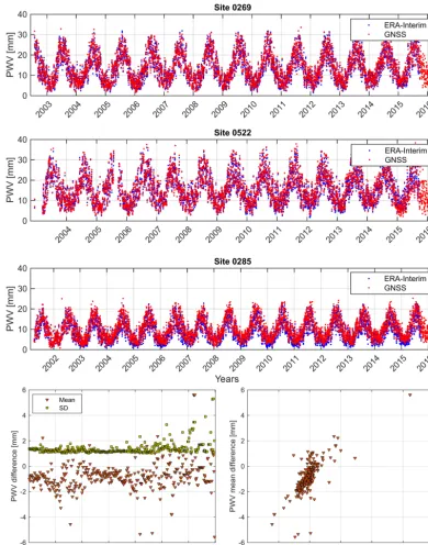
We compared the PWV obtained from GNSS with ERA-Interim data. Figure 2 shows the results for three sites at dif-ferent altitudes as well as the mean and standard deviations of the time series difference. ERA-Interim grid provides val-ues of PWV at grid points separated by about 79 km in lon-gitude and latitude. The ECMWF provides software to hori-zontally interpolate the current ERA-Interim grid at different locations of the GNSS stations as described in Heise et al. (2009). We did not account for altitude difference, which has a significant impact in mountainous areas. For the sites lo-cated in flat terrain, the two data sets show strong correlation with the bias values below 1 mm and standard deviation of less than 2 mm (Fig. 2). The bias between the data sets in-creases for sites in mountainous regions. The time series of the site 0285 (Garmisch, Germany; 1779 m a.m.s.l.), for ex-ample, show a larger bias between GNSS and ERA-Interim data, which is explained as follows: we average PWV of four distant grid points around the GNSS site. With the rough spa-tial resolution, the variability of surface topography is not well captured in the reanalysis data, which significantly in-creases the height difference between GNSS and the model, and hence the PWV difference. Additionally, the daily mean in ERA-Interim is obtained by averaging four PWV values per day, while using GNSS there are 96 PWV estimates per day. This positive bias was also observed by Morland et al. (2006) and Sussmann and Camy-Peyret (2002, 2003) when comparing ERA 40 and GPS in the Alps for the site Jungfrau-joch at 3584 m a.m.s.l.
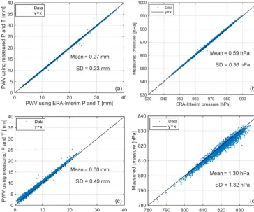
For accurate determination of the PWV from GNSS mea-surements, it is required to have measurements of mainly air pressure and temperature at the GNSS sites or within a short spatial range. In the absence of meteorological mea-surements, would the interpolation of pressure and tempera-ture from reanalysis data be a good replacement? To answer this question, we compared the PWV time series extracted from the ZTD by using both measurements at the meteoro-logical stations and ERA-Interim data. To calculate the ZHD, the in situ measured pressure and temperature are horizon-tally interpolated to the GNSS site and then vertically inter-polated to the GNSS antenna phase center. For GNSS sites below the lowest ERA-Interim level, the pressure and tem-perature are extrapolated at the site altitude as described in Heise et al. (2009). The ZWD is then extracted and con-verted into PWV. Figure 3 shows the scatterplots of PWV obtained using surface measurements and ERA-Interim data. We found that in regions of smooth topography, the ERA-Interim data and the measurements provide almost the same values of PWV and pressure. In regions of steep topographic
gradients, however, the ERA-Interim data show slightly dif-ferent results, which is mainly related to the pressure data as observed from Fig. 3. The deviations between the measured pressure and the ERA-Interim pressure increase in mountain-ous regions, which affects the calculation of the ZHD and hence the obtained PWV.
Besides station pressure, an important factor for an accu-rate determination of PWV is the conversion factor5, which should be calculated using measurements of surface temper-ature. Askne and Nordius (1987) determined the conversion factor5as follows:
5= 10 6
ρwRw
k3
Tm+k
0
2
, (6)
whereρw is the density of water andRwis the specific gas constant of water vapor (461.5 J kg−1K−1). In our research, we used the values of the physical constantsk3andk20 given by Bevis et al. (1994),Tmwas given by Davis et al. (1985) as
Tm= R
z Pwv
T dz R
z Pwv
T2 dz
, (7)
whereT is the air temperature andPwvwater vapor pressure at vertical levels. Davis et al. (1985) suggested the use of wa-ter vapor pressure and temperature profiles from radioson-des; however, it is easier to get these profiles from numeri-cal atmospheric models. In this work, we obtainedTmas de-scribed in Heise et al. (2009) using the ERA-Interim model that covers 60 vertical levels extending from the Earth’s sur-face up to 0.1 hPa.Tmcan be well approximated based on air surface temperature by the following formula (Bevis et al., 1992):
Figure 2.PWV estimated at three GNSS sites (site 0269 in Wertach, Germany, at altitude of 907 m a.m.s.l.; site 0522 in Pirmasens, Germany, at altitude of 399 m a.m.s.l.; and site 0285 in Garmisch, Germany, at altitude of 1779 m a.m.s.l.) and the corresponding PWV from ERA-Interim. The bottom sub-figures show (left) the mean of PWV difference (ERA-Interim–GNSS) and (right) the standard deviation at all sites.
by computing the PWV using the two different values of
Tm, the results show a bias of 0.048 mm for site 0522 and −0.083 mm for site 0285. Hence, Eq. (8) will be used to cal-culateTmsince it only requires the measured surface temper-ature.
3 Decadal variability in time series of atmospheric variables
3.1 Estimating the trend using least squares regression
fore-Figure 3. (a, c)PWV determined using interpolated pressure and temperature from surface measurements and ERA-Interim and the corre-sponding pressure values for the GNSS site 0522. Similarly in panels(b, d)for the GNSS site 0285.
Figure 4.Mean atmospheric temperature,Tm, determined once using surface temperature and vertical atmospheric profiles from
ERA-Interim at the sites 0522 (399 m a.m.s.l.) and 0285 (1779 m a.m.s.l.). The bias is 0.97 K for the first site and 3.02 for the second, and the SD is 2 K for the first and for the second 1.83 K.
casting economic data. The method was to decompose the time series into a trend, a seasonal, a cyclic, and an irregular component (Enders, 1995). The trend component represents the long-term behavior of the time series, while the seasonal and the cyclic components represent the regular and periodic movements. The time series also contain a stochastic
irreg-ular component. Time series of PWV and temperature, for example, have different temporal variations that can be rea-sonably modeled using this approach. Here holds an additive model, such that the time seriesyt can be extended as
whereTt is a deterministic trend component with slow tem-poral variations,St represents the seasonal component with known periodicity (e.g., 12 months for PWV and tempera-ture), and It represents the irregular (stationary) stochastic component with short temporal variations. We did not ob-serve a regular signal that lasts longer than 1 year, so we ex-cluded the cyclic component for the model. The presence of seasonality might mask the small changes in the linear trend. Therefore, for proper trend analysis, the seasonal component has to be estimated and removed from the time series, which is known by seasonal adjustment (Enders, 1995). The desea-sonalized data are useful for extracting the long-term trend and exploring the irregular component of a time series.
The seasonal adjustment is applied as an iterative proce-dure as follows. To best estimate the seasonal component, the linear trend has first to be estimated and removed from the time series. There are different methods to estimate the trend such as using moving average or parametric trend estimation. Here, we used the method of moving average with a window length of 1 year that is able to smooth out seasonal and irreg-ular signals. We employ time series of PWV and temperature with daily values (the GNSS-based estimates of PWV have a temporal resolution of 15 min, but we average them to get mean daily values for climatological studies). The trend is estimated as follows:
ˆ
Tt=
yt−q+yt−q+1+ · · · +yt+q−1+yt+q
d . (10)
Since the time series are daily and the seasonal signal is an-nual, the value ofd is 365 andq=(d−1)/2. Ford=366,
q=d/2 and the trend is estimated from ˆ
Tt=
0.5yt−q+yt−q+1+ · · · +yt+q−1+0.5yt+q
d . (11)
The estimated trend component is subtracted from the original time series and the detrended signal is averaged to estimate the seasonal componentSˆt as follows. We first ob-tain
wt =
1
number of summands n−q−t
d X
q−t d
(yt+j d− ˆTt+j d), (12)
withnthe number of data samples. Thenwtis centered, i.e., we derive a seasonal signal with a zero mean.
ˆ
St =wt− 1
d
d X
k=1
wk, t=1,2,· · ·, d (13)
For an additive model, Sˆt should fluctuate around zero to avoid any influence from the trend. The estimated seasonal component is subtracted from the original time series to ob-tain a seasonally adjusted time seriesdyt, i.e.,
dyt=yt− ˆSt. (14)
Figure 5 shows an example of the trend, seasonal, and irreg-ular components of PWV time series at site 0896 in Berlin. To estimate the slope of the trend, we fit a straight line
ˆ
T = ˆb+ ˆm tto the trend component produced by the moving average step. The standard deviation of the estimated slope (called standard error) is calculated as (Wigley et al., 2006)
sm2ˆ = 1 n−2
Pn
1(yi− ˆy)2 Pn
1(ti− ¯t )2
, (15)
wheren−2 is the degree of freedom forndata points. The ap-proximate 95 % confidence interval is expressed asmˆ±2smˆ.
Weatherhead et al. (1998) presented another way to calculate the standard deviation of the estimated slope.
sm∗ˆ = σI
n
3 2
y s
1+φI 1−φI
, (16)
whereσIdenotes the standard deviation of the irregular com-ponent andny denotes the number of years of the data. φI represents the one-lag autocorrelation of the irregular com-ponent.
3.2 Estimating the trend using Theil–Sen estimator The Theil–Sen estimator presented by Theil (1950) and Sen (1968) aims to robustly find the linear fit of a data set despite containing outliers. If(t1, y1),. . .,(tn, yn)represent the data points, then the Theil–Sen estimator determines the slope of the line that connects each data pair. The median among the slopes of all pairs in the slope of the fit, i.e.,
ˆ
m=median y
j−yi
tj−ti
for i < j≤n. (17)
Figure 5.Trend, seasonal, and irregular components of PWV time series estimated from GNSS observations (2001–2016) at the site 0896 (Berlin, Germany; 68.37 m a.m.s.l.).
Table 1.Comparison between the estimated trends (mm decade−1) from radiosonde, dew-point-based, and ERA-Interim PWV time se-ries at site Lindenberg. The standard error of the estimated trend is ≈0.04 mm decade−1.
Method Radiosonde Dew point ERA-based Interim
Least squares 0.533 0.503 0.461 Theil–Sen 0.512 0.533 0.482
We also analyze the change in PWV in relation to the change in temperature. As temperature rises, the air capacity to hold moisture increases at the Clausius–Clapeyron rate. The water vapor pressure e is related to temperature T as follows: e2 e1 =exp 1H v R 1 T1 − 1 T2 , (18)
where1Hvis enthalpy of vaporization andRis the universal gas constant. This relationship indicates that 1°C rise in the temperature increases the vapor pressure by 7 %. Based on this formula, the change in the PWV can theoretically be re-lated to the change in the temperature. The PWV is linearly related to the vapor pressure as presented in Tuller (1977), i.e., PWV=2.3e. By substituting this into Eq. (18), the in-crement in PWV should, in theory, be the same as the incre-ment in the vapor pressure (approximately 7 %) per degree Celsius rise in temperature. This was also observed by ana-lyzing the temperature, water vapor pressure, and PWV data sets. We obtained the change in PWV and vapor pressure per 1◦rise in temperature as shown in Fig. 12. The increase in the water vapor pressure at 227 stations is in the range of 4.5 and 6.5 %, which is close to the Clausius–Clapeyron rate. We observed a similar rate of change for the PWV with the temperature, or more precisely, PWV2
PWV1 =1.003
e2
e1.
4 Results
4.1 Estimating the trends using GNSS-based PWV In this section, we show the estimated trends using three data sets, GNSS, ERA-Interim, and synoptic data of PWV and temperature. First, we estimated the trends of PWV at 351 GNSS sites with time series of 4 to 19 years long and the corresponding standard deviations of the estimated slope as shown in Fig. 7. The size of the marker is proportional to the length of the time series (small squares indicate short time series). As observed from the figure, there are high trend val-ues, particularly at sites with short time series. Therefore, in Fig. 8a, we eliminated all sites with time series shorter than 10 years. At the remaining 119 sites the PWV trend varies be-tween−1.5 and 2.3 mm decade−1(except for six sites) with precision of the estimated trends below 0.25 mm decade−1.
To validate these estimates, we analyzed ERA-Interim data over the same times where GNSS data are available (Fig. 8c). The results from concurrent ERA-Interim time series show high similarity in the trend values and the variations of the trend in space.
4.2 Estimating the trends using longer time series Since the trend is estimated from GNSS time series of dif-ferent length, it is reasonable to provide a mean value for the whole region or observe spatial features of the trends. There-fore, and in order to get more insight and more reasonable conclusions about the long-term temporal variations of PWV, it is necessary to analyze time series spanning one predefined period for all stations. Since the last climate normal extends from 1991 to 2020, we analyzed time series of 26 years (Jan-uary 1991–June 2016) from ERA-Interim and synoptic data. We investigated time series at 227 meteorological stations where the ERA-Interim is horizontally interpolated at the synoptic station using bilinear interpolation. Figure 9 shows the estimated trends using ERA-Interim PWV time series by, first, applying the least squares to the seasonally adjusted data and, second, using the Theil–Sen method. Both meth-ods show similar values of the trend, positive with values of 0.34±0.06 mm decade−1. As observed from Fig. 9, the trend tends to increase in the direction to northeastern Germany.
In order to validate these results, it is necessary to have a long data set, which is not available for this research. How-ever, DWD provides surface measurements of atmospheric parameters that are accurate and homogenous so that they are proper for climate studies. It is not possible to accurately determine the total column water vapor using surface me-teorological observations alone. However, it was shown in the 1960s that it is possible to approximate the atmospheric PWV based on dew point temperature measurements, which is considered an indicator of the amount of moisture in the air (Reitan, 1963). The dew point temperature in turn is de-termined based on the air temperature and relative humid-ity. Reitan (1963) presented a basic relationship between the mean monthly PWV and mean monthly surface dew point temperature by the following regression form:
PWV=exp(bTd+a), (19)
where PWV is in centimeters andTdis the dew point temper-ature in degrees Fahrenheit.aandbare estimated to have the values of−0.981 and 0.0341 (Reitan, 1963). The standard error in the PWV estimate was 0.18 cm. Following the same procedure, Bolsenga (1965) obtained slightly different esti-mates foraandbusing hourly and mean daily observations. Smith (1966) obtained a similar regression equation with the coefficienta not being constant. It depends on the vertical distribution of the atmospheric moisture, i.e.,
PWV=exp
0.0393 | {z }
b
Td+[0.1133−ln(λ+1)]
| {z }
a
Figure 7.The estimated PWV trend at 351 GNSS sites and the corresponding uncertainty in the estimated trend using Theil–Sen estimator. The size of the marker indicates the length of the PWV time series; i.e., the larger the marker, the longer time series.
Figure 9.The estimated PWV trend using (2 m) ERA-Interim data by applying least squares regression to the seasonally adjusted time series(a)and Theil–Sen estimator(c). The standard errors of the estimated trends are shown in panels(b, d).
with the value of λ dependent on the site latitude and the season of year (Smith, 1966).
In this work, we estimated the coefficientsaandbat each meteorological station by fitting the curves in Eq. (19) to the ERA-Interim PWV data. The median values fora andb us-ing daily PWV are−1.346 and 0.039, which are close to the values−1.249 and 0.0427 presented by Bolsenga (1965). For monthly PWV, the median values are−1.224 and 0.037 for
aandb, respectively.
We used measurements of surface dew point temperature to obtain the daily PWV and time series for the whole net-work are evaluated using the ERA-Interim data. The PWV value at the meteorological station is computed by applying bilinear interpolation to the ERA-Interim PWV at four grid points around that station. The altitude difference was not accounted for. Figure 10a shows the bias and standard de-viation values of daily PWV for 227 stations as well as the bias against the altitude difference of the two data sets
(ERA-Interim height−station height). The bias is centered around 0.15 mm and the standard deviation around 2.5 mm. From Fig. 10b we observe that the higher the altitude difference, the larger is the mean PWV difference.
Figure 10. (a)Mean and standard deviation of the PWV time series difference (1991–2016) from ERA-Interim and synoptic data at 227 sta-tions.(b)Mean of PWV difference (ERA-Interim–synoptic) against the altitude difference.
Figure 11.Estimated trends using dew-point-based PWV and the corresponding standard error of the estimated slope.
The same procedure is applied to estimate the trends from temperature and dew point temperature time series. The estimated temperature trends from surface measure-ments at 227 stations shown in Fig. 13a fluctuate in the range of 0.39±0.1 K decade−1. In Fig. 13c the trend
Figure 12.The increase in atmospheric water vapor pressure and PWV per 1◦Celsius rise in temperature using data at 227 stations.
and 6.5 %, which is comparable to the theoretical rate of the Clausius–Clapeyron equation.
Also, the estimated trend in PWV is correlated with that from the dew point temperature, which is exhibited in Fig. 13c. Using ERA-Interim temperature and dew point temperature leads to the same observation; however, the trend values are slightly different. We also observed that the trends of dew point temperature are almost in the same range as those for PWV, which makes time series of the dew point temperature proper to provide reasonably adequate informa-tion about PWV trends.
5 Conclusions
In this paper, we aimed at estimating climatic trends from GNSS-based precipitable water vapor time series and sur-face measurements of air temperature in Germany. First, we compared PWV time series obtained from GNSS and ERA-Interim, which show strong correlation with an average bias of −1.7 mm (ERA-Interim–GNSS) and standard deviations of 2.63 mm.
By comparing the GNSS-based PWV with those from ERA-Interim, the results show small bias values in flat ter-rain, while the bias increases in mountainous regions. This is mostly caused by the coarse spatial resolution of the ERA-Interim data and hence the inability to properly represent the topography.
To evaluate the temporal evolution of PWV and temper-ature, we modeled the time series with an additive model that contains trend, seasonal, and stochastic irregular com-ponents. The time series are seasonally adjusted to remove the periodic signal, and the trend component is then an-alyzed after filtering out the irregular component caused mainly by weather variations. The comparison of this method with the Theil–Sen estimator shows insignificant differ-ences in the estimated trends. The GNSS-based estimated PWV trends change between−1.5 and 2.3 mm decade−1for time series that are 10 to 19 years long. Since the PWV time series at different GNSS sites are not concurrent, we could not draw specific conclusions about the mean trend or spatial features of the trend over the whole research re-gion. Therefore, we extended the research to analyze 26-year (1991–2016) time series from ERA-Interim and syn-optic stations. Using dew point temperature, we could pro-duce PWV time series at 227 stations with a bias below 1.2 mm to the ERA-Interim data. By analyzing time se-ries of 26 years from ERA-Interim and synoptic data, the PWV trends are observed to be positive and in the range of 0.34±0.06 and 0.48±0.13 mm decade−1, respectively. The ERA-Interim PWV shows lower trend values of the trend. We found that the trends estimated, using 26 years of data for each station, tend to show a positive gradient when mov-ing from southwestern to northeastern Germany. This was
observed in ERA-Interim and synoptic data for both PWV and temperature time series.
The increment in PWV varies between 4.5 and 6.5 % per degree Celsius rise in temperature, which is comparable to the theoretical rate of the Clausius–Clapeyron equation. The magnitude of the PWV trend slightly differs from that of the dew point temperature. Hence, we can consider the trends estimated from the dew point temperature as a measure for the PWV trends in case of lack of observations.
It would be illuminating to validate the results of this re-search using a data set that has a higher spatial resolution than the ERA-Interim.
Data availability. In this paper, we used (1) ERA-Interim data, which can be downloaded from the ECMWF servers (http://apps. ecmwf.int/datasets/data/interim-full-daily/levtype=sfc/; Dee et al., 2011); and (2) synoptic data, which can be downloaded from the DWD data center ftp://ftp-cdc.dwd.de/pub/CDC/. The GNSS-based data can be acquired by sending a request to the GFZ.
Competing interests. The authors declare that they have no conflict of interest.
Acknowledgements. The authors would like to thank the ECMWF for making publicly available the ERA-Interim data. Thanks also go to the German Meteorological Service (DWD) for providing us with hourly meteorological measurements.
The article processing charges for this open-access publication were covered by a Research
Centre of the Helmholtz Association.
Edited by: Ralf Sussmann
Reviewed by: two anonymous referees
References
Alshawaf, F., Hinz, S., Mayer, M., and Meyer, F. J.: Constructing accurate maps of atmospheric water vapor by combining inter-ferometric synthetic aperture radar and GNSS observations, J. Geophys. Res.-Atmos., 120, 1391–1403, 2015.
Arguez, A. and Vose, R. S.: The definition of the standard WMO climate normal: The key to deriving alternative climate normals, B. Am. Meteorol. Soc., 92, 699–704, 2011.
Askne, J. and Nordius, H.: Estimation of tropospheric delay for mi-crowaves from surface weather data, Radio Sci., 22, 379–386, 1987.
Bender, M., Dick, G., Wickert, J., Schmidt, T., Song, S., Gendt, G., Ge, M., and Rothacher, M.: Validation of GPS slant delays using water vapour radiometers and weather models, Meteorol. Z., 17, 807–812, 2008.
vapour tomography system using algebraic reconstruction tech-niques, Adv. Space Res., 47, 1704–1720, 2011.
Bengtsson, L., Hagemann, S., and Hodges, K. I.: Can climate trends be calculated from reanalysis data?, J. Geophys. Res.-Atmos., 109, D11111, https://doi.org/10.1029/2004JD004536, 2004. Bennitt, G. V. and Jupp, A.: Operational assimilation of GPS zenith
total delay observations into the met office numerical weather prediction models, Mon. Weather Rev., 140, 2706–2719, 2012. Bevis, M., Businger, S., Herring, T. A., Rocken, C., Anthes, R. A.,
and Ware, R. H.: GPS Meteorology: Remote sensing of atmo-spheric water vapor using the global positioning system, J. Geo-phys. Res.-Atmos., 97, 15787–15801, 1992.
Bevis, M., Businger, S., Chiswell, S., Herring, T. A., Anthes, R. A., Rocken, C., and Ware, R. H.: GPS Meteorology: Mapping Zenith Wet Delays onto Precipitable Water, J. Appl. Meteorol., 33, 379–386, 1994.
Bock, O., Keil, C., Richard, E., Flamant, C., and Bouin, M.-N.: Val-idation of precipitable water from ECMWF model analyses with GPS and radiosonde data during the MAP SOP, Q. J. Roy. Me-teor. Soc., 131, 3013–3036, 2005.
Bolsenga, S. J.: The relationship between total atmospheric water vapor and surface dew point on a mean daily and hourly basis, J. Appl. Meteorol., 4, 430–432, 1965.
Davis, J., Herring, T., Shapiro, I., Rogers, A., and Elgered, G.: Geodesy by radio interferometry: Effects of atmospheric model-ing errors on estimates of baseline length, Radio Sci., 20, 1593– 1607, 1985.
Davis, J. L.: Atmospheric Propagation Effects on Radio Interfer-ometry, PhD dissertation, Massachusetts Institute of Technology, Cambridge, MA, USA, Scientific Report No. 1, AFGL-TR-86-0243, 276 pp., 1986.
Dee, D. P., Uppala, S. M., Simmons, A. J., Berrisford, P., Poli, P., Kobayashi, S., Andrae, U., Balmaseda, M. A., Balsamo, G., Bauer, P., Bechtold, P., Beljaars, A. C. M., van de Berg, L., Bid-lot, J., Bormann, N., Delsol, C., Dragani, R., Fuentes, M., Geer, A. J., Haimberger, L., Healy, S. B., Hersbach, H., Holm, E. V., Isaksen, L., Kallberg, P., Köhler, M., Matricardi, M., McNally, A. P., Monge-Sanz, B. M., Morcrette, J.-J., Park, B.-K., Peubey, C., de Rosnay, P., Tavolato, C., Thepaut, J.-N., and Vitart, F.: The ERA-Interim reanalysis: Configuration and performance of the data assimilation system, Q. J. Roy. Meteor. Soc., 137, 553–597, 2011.
Elgered, G. and Jarlemark, P. O.: Ground-based microwave radiom-etry and long-term observations of atmospheric water vapor, Ra-dio Sci., 33, 707–717, 1998.
Enders, W.: Applied Econometric Time Series, Wiley, New York, USA, 1995.
Gendt, G., Dick, G., Reigber, C., Tomassini, M., Liu, Y., and Ra-matschi, M.: Near real time GPS water vapor monitoring for nu-merical weather prediction in germany, J. Meteor. Soc. Jpn., 82, 361–370, 2004.
Gradinarsky, L., Johansson, J., Bouma, H., Scherneck, H.-G., and Elgered, G.: Climate monitoring using GPS, Phys. Chem. Earth Pt. A/B/C, 27, 335–340, 2002.
Haas, R., Elgered, G., Gradinarsky, L., and Johansson, J. M.: As-sessing long term trends in the atmospheric water vapor content by combining data from VLBI, GPS, radiosondes and microwave radiometry, in: Proceedings of the 16th Working Meeting on Eu-ropean VLBI for Geodesy and Astrometry, edited by:
Schweg-mann, W. and Thorandt, V., Bundesamt für Kartographie und Geodäsie, 9–10 May 2003, Frankfurt/Leipzig, Germany, 279– 288, 2003.
Hausmann, P., Sussmann, R., Trickl, T., and Schneider, M.: A decadal time series of water vapor and D/H isotope ratios above Zugspitze: transport patterns to central Europe, Atmos. Chem. Phys., 17, 7635–7651, https://doi.org/10.5194/acp-17-7635-2017, 2017.
Heise, S., Dick, G., Gendt, G., Schmidt, T., and Wickert, J.: Inte-grated water vapor from IGS ground-based GPS observations: initial results from a global 5-min data set, Ann. Geophys., 27, 2851–2859, https://doi.org/10.5194/angeo-27-2851-2009, 2009. Jade, S. and Vijayan, M.: GPS-based atmospheric precipitable water vapor estimation using meteorological parameters interpolated from NCEP global reanalysis data, J. Geophys. Res.-Atmos., 113, D03106, https://doi.org/10.1029/2007JD008758, 2008. Luo, X., Mayer, M., and Heck, B.: Extended neutrospheric
mod-elling for the GNSS-based determination of high-resolution at-mospheric water vapor fields, Bol. Cienc. Geod., 14, 149–170, 2008.
Morland, J., Liniger, M., Kunz, H., Balin, I., Nyeki, S., Mätzler, C., and Kämpfer, N.: Comparison of GPS and era40 iwv in the alpine region, including correction of GPS observations at Jungfraujoch (3584 m), J. Geophys. Res.-Atmos., 111, D04102, https://doi.org/10.1029/2005JD006043, 2006.
Nilsson, T. and Elgered, G.: Long-term trends in the at-mospheric water vapor content estimated from ground-based gps data, J. Geophys. Res.-Atmos., 113, D19101, https://doi.org/10.1029/2008JD010110, 2008.
Ning, T., Wickert, J., Deng, Z., Heise, S., Dick, G., Vey, S., and Schöne, T.: Homogenized time series of the atmospheric wa-ter vapor content obtained from the GNSS reprocessed data, J. Climate, 29, 2443–2456, https://doi.org/10.1175/JCLI-D-15-0158.1, 2016.
Pichelli, E., Ferretti, R., Cimini, D., Perissin, D., Montopoli, M., Marzano, F. S., and Pierdicca, N.: Water vapour distribution at urban scale using high-resolution numerical weather model and spaceborne SAR interferometric data, Nat. Hazards Earth Syst. Sci., 10, 121–132, https://doi.org/10.5194/nhess-10-121-2010, 2010.
Reitan, C. H.: Surface dew point and water vapor aloft, J. Appl. Meteorol., 2, 776–779, 1963.
Rienecker, M. M., Suarez, M. J., Todling, R., Bacmeister, J., Takacs, L., Liu, H., Gu, W., Sienkiewicz, M., Koster, R., Gelaro, R., Sta-jner I., and Nielsen J. E.: The GEOS-5 data assimilation system-documentation of versions 5.0. 1, 5.1. 0, and 5.2. 0. Technical Report Series on Global Modeling and Data Assimilation, Vol-ume 27, NASA Goddard Space Flight Center, Greenbelt, Mary-land, USA, 2008.
Saastamoinen, J.: Contributions to the theory of atmospheric refrac-tion, B. Géod., 107, 13–34, 1973.
Sen, P. K.: Estimates of the regression coefficient based on Kendall’s tau, J. Am. Stat. Assoc., 63, 1379–1389, 1968. Simmons, A., Uppala, S., Dee, D., and Kobayashi, S.: ERA-Interim:
New ECMWF reanalysis products from 1989 onwards, ECMWF Newsl., 110, 29–35, 2007.
Sussmann, R. and Camy-Peyret, C.: Ground-Truthing Center Zugspitze, Germany for AIRS/IASI validation, Phase I Report, EUMETSAT, 18 pp., available at: http://www.imk-ifu.kit.edu/ downloads/AIRSVAL_Phase_I_Report.pdf (last access: 11 July 2017), 2002.
Sussmann, R. and Camy-Peyret, C.: Ground-Truthing Center Zugspitze, Germany for AIRS/IASI validation, Phase II Report, EUMETSAT, 15 pp., available at: http://www.imk-ifu.kit.edu/ downloads/AIRSVAL_Phase_II_Report.pdf (last access: 11 July 2017), 2003.
Theil, H.: A rank-invariant method of linear and polynomial regres-sion analysis, 1, 2, and 3, Nederl. Akad. Wentsch Proc., 53, 386– 392, 1950.
Tuller, S. E.: The relationship between precipitable water vapor and surface humidity in New Zealand, Arch. Meteor. Geophy. A, 26, 197–212, 1977.
Vey, S., Dietrich, R., Fritsche, M., Rülke, A., Steigenberger, P., and Rothacher, M.: On the homogeneity and interpreta-tion of precipitable water time series derived from global GPS observations, J. Geophys. Res.-Atmos., 114, D10101, https://doi.org/10.1029/2008JD010415, 2009.
Wang, X. J.: Maximizing correlation in the presence of missing data, Applied Mathematical Sciences, 2, 2653–2664, 2008. Weatherhead, E. C., Reinsel, G. C., Tiao, G. C., Meng, X.-L., Choi,
D., Cheang, W.-K., Keller, T., DeLuisi, J., Wuebbles, D. J., Kerr, J. B., Miller A. J., Oltmans S. J., and Frederick J. E.: Factors affecting the detection of trends: Statistical considerations and applications to environmental data, J. Geophys. Res., 103, 17– 149, 1998.
Wigley, T. M., Santer, B., and Lanzante, J.: Appendix a: Statistical issues regarding trends, in: Temperature trends in the lower at-mosphere: steps for understanding and reconciling differences. A Report by the Climate Change Science Program and the Sub-committee on Global Change Research, Washington, DC, USA, 129–139, 2006.