Comparison of ERA5 and ERA-Interim near-surface air temperature, snowfall and precipitation over Arctic sea ice: effects on sea ice thermodynamics and evolution

(1)

The Cryosphere, 13, 1661–1679, 2019 https://doi.org/10.5194/tc-13-1661-2019

Comparison of ERA5 and ERA-Interim near-surface air

temperature, snowfall and precipitation over Arctic sea ice:

effects on sea ice thermodynamics and evolution

Caixin Wang1,2, Robert M. Graham2, Keguang Wang1, Sebastian Gerland2, and Mats A. Granskog2

1_{Department of Research and Development, Norwegian Meteorological Institute, 9293 Tromsø, Norway} 2_{Research Department, Fram Centre, Norwegian Polar Institute, P.O. Box 6606 Langnes, 9296 Tromsø, Norway}

Correspondence:Caixin Wang (caixin.wang@npolar.no)

Received: 12 November 2018 – Discussion started: 7 December 2018 Revised: 7 May 2019 – Accepted: 29 May 2019 – Published: 14 June 2019

Abstract.Rapid changes are occurring in the Arctic, includ-ing a reduction in sea ice thickness and coverage and a shift towards younger and thinner sea ice. Snow and sea ice mod-els are often used to study these ongoing changes in the Arc-tic, and are typically forced by atmospheric reanalyses in ab-sence of observations. ERA5 is a new global reanalysis that will replace the widely used ERA-Interim (ERA-I). In this study, we compare the 2 m air temperature (T2M), snowfall (SF) and total precipitation (TP) from ERA-I and ERA5, and evaluate these products using buoy observations from Arctic sea ice for the years 2010 to 2016. We further assess how biases in reanalyses can influence the snow and sea ice evo-lution in the Arctic, when used to force a thermodynamic sea ice model. We find that ERA5 is generally warmer than ERA-I in winter and spring (0–1.2◦C), but colder than ERA-I in summer and autumn (0–0.6◦C) over Arctic sea ice. Both reanalyses have a warm bias over Arctic sea ice relative to buoy observations. The warm bias is smaller in the warm season, and larger in the cold season, especially when the T2M is below−25◦C in the Atlantic and Pacific sectors. In-terestingly, the warm bias for ERA-I and new ERA5 is on av-erage 3.4 and 5.4◦C (daily mean), respectively, when T2M is lower than −25◦C. The TP and SF along the buoy tra-jectories and over Arctic sea ice are consistently higher in ERA5 than in ERA-I. Over Arctic sea ice, the TP in ERA5 is typically less than 10 mm snow water equivalent (SWE) greater than in ERA-I in any of the seasons, while the SF in ERA5 can be 50 mm SWE higher than in ERA-I in a sea-son. The largest increase in annual TP (40–100 mm) and SF (100–200 mm) in ERA5 occurs in the Atlantic sector. The SF to TP ratio is larger in ERA5 than in ERA-I, on average

0.6 for ERA-I and 0.8 for ERA5 along the buoy trajectories. Thus, the substantial anomalous Arctic rainfall in ERA-I is reduced in ERA5, especially in summer and autumn. Simu-lations with a 1-D thermodynamic sea ice model demonstrate that the warm bias in ERA5 acts to reduce thermodynamic ice growth. The higher precipitation and snowfall in ERA5 results in a thicker snowpack that allows less heat loss to the atmosphere. Thus, the larger winter warm bias and higher precipitation in ERA5, compared with ERA-I, result in thin-ner ice thickness at the end of the growth season when using ERA5; however the effect is small during the freezing period.

1 Introduction

(2)

driven in part by an increased number of storms that bring warm winds from the south (Woods and Caballero, 2016; Dahlke and Maturilli, 2017; Graham et al., 2017a, b; Rinke et al., 2017). The additional heat and moisture carried by these storms could contribute to a reduction in the winter ice growth (Woods and Caballero, 2016; Alexeev et al., 2017; Stroeve et al., 2018).

Despite the rapid ongoing changes in the Arctic, there are relatively few direct observations of the atmosphere, sea ice and ocean conditions, especially during winter. Due to the lack of in situ observations, most studies documenting changes in the Arctic rely heavily on atmospheric reanalyses (Screen and Simmonds, 2010; Kapsch et al., 2014; Woods and Caballero, 2016; Sato and Inoue, 2017). In addition, re-analyses are also frequently used to force snow and sea ice models (Schweiger et al., 2011; Merkouriadi et al., 2017; Stroeve et al., 2018). However, there are inherent biases and uncertainties within these reanalyses, and large differences can exist among the different products (Tjernstöm and Gra-versen, 2009; Decker, et al., 2012; Jakobson et al., 2012; Lindsay et al., 2014; Wesslén et al., 2014; Graham et al., 2017b). Thus the choice of reanalysis, and inherent biases within that product, will ultimately influence the simulation of Arctic sea ice mass balance (Cheng et al., 2008; Wang et al., 2015).

The European Centre for Medium-range Weather Fore-casts (ECMWF) reanalysis product, ERA-Interim (ERA-I; Dee et al., 2011), has been widely used for studying changes in the Arctic and forcing ocean and sea ice models (e.g. Cheng et al., 2008; Maksimovich and Vihma, 2012; Kap-sch et al., 2014; Woods and Caballero, 2016; Graham et al., 2017b). In 2017, the ECMWF released a new reanaly-sis ERA5 (Hersbach and Dee, 2016). There are several ma-jor improvements in ERA5 compared with ERA-I, includ-ing much higher spatial and temporal resolutions, and more consistent sea surface temperature and sea ice concentration (Hersbach and Dee, 2016). Evaluations of the performance of ERA5 have been conducted over land and revealed a higher performance of ERA5 than ERA-I (Albergel et al., 2018; Ur-raca et al., 2018), and other commonly used reanalyses, such as, MERRA-2 (the second version of the Modern-Era Retro-spective Analysis for Research and Applications) (Olausen, 2018; Urraca et al., 2018). However, the performance of ERA5 over Arctic sea ice is yet to be fully investigated.

In this study, we compare and evaluate the performance of ERA-I and ERA5 over Arctic sea ice. For this, we use data from ice mass balance buoys (IMBs) (Perovich et al., 2017) and snow buoys (Grosfeld et al., 2016; Nicolaus et al., 2017) deployed from 2010 to 2015. The buoys record position, the 2 m air temperature (T2M), mean sea level pressure (MSLP) and snow depth at regular intervals. Hence, these observa-tions can be used to evaluate the variables of T2M, precipi-tation and MSLP in the reanalyses. The former two variables are critical parameters for sea ice simulation (Cheng et al., 2008; Wang et al., 2015), and form the focus of our study. We

use the T2M and snow depth observations from these buoys to assess the performance of ERA5 and ERA-I over Arctic sea ice. We further use the reanalyses to force a 1-D thermo-dynamic sea ice model. The simulations are compared with snow and ice thickness observations from the buoys to eval-uate how differences in the T2M and precipitation influence the evolution of sea ice in the model.

2 Materials and methods 2.1 Buoy data

IMBs autonomously measure thermodynamic changes in sea ice mass balance (Richter-Menge et al., 2006; Polashenski et al., 2011). They are part of a network of drifting buoys over the Arctic Ocean that provide meteorological and oceano-graphic data for real-time operational requirements and re-search purposes (Rigor et al., 2000). These instruments typi-cally record GPS position, T2M and mean sea level pressure (MSLP) at hourly intervals, as well as temperature profiles through the air, snow, ice, and upper-ocean and distances to snow/ice surface and ice bottom at 4 h intervals. Snow depth and ice thickness can be estimated from the distances mea-sured by acoustic sounders, if the initial thickness of snow and ice is known when the IMB is deployed (Wang et al., 2013). If the acoustic sounders fail but the temperature string works, the positions of the ice surface and bottom can be determined from the temperature readings. Similar to IMBs, snow buoys also record GPS position, T2M, MSLP and snow depth at hourly intervals (Grosfeld et al., 2016; Nicolaus et al., 2017). However, snow buoys do not measure temperature profiles, and provide no information on ice thickness.

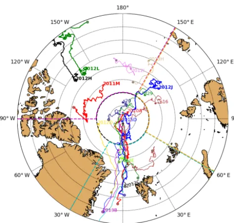
Since 2000, a large number of IMBs have been deployed across the Arctic, in regions such as the central Arctic, the Beaufort Sea, the Chukchi Sea, the Laptev Sea, the North Pole, Canadian Islands and Svalbard (Perovich et al., 2017; http://imb-crrel-dartmouth.org/archived-data/, last ac-cess: 15 October 2017). In this study, we use data from 13 IMBs deployed in these different regions between 2010 and 2015 (Fig. 1, Table 1). The IMBs were typically de-ployed in the central Arctic during April–May, while deploy-ments in the Beaufort, Laptev and Chukchi seas generally took place in August–September (Fig. 1, Table 1). For ad-ditional coverage, we also use observations from three snow buoys deployed in 2015, two of which were in the Laptev Sea and one in the central Arctic (Table 1; Fig. 1) (http: //www.meereisportal.de/en, last access: 17 January 2018). For simplicity, hereafter we refer to IMBs and snow buoys as buoys.

2.2 ERA5 and ERA-I reanalysis data

(3)

C. Wang et al.: Comparison of ERA5 and ERA-Interim over Arctic sea ice 1663

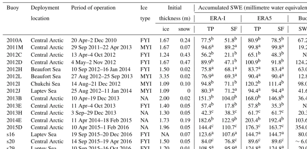
Table 1.Summary of deployment locations and initial conditions for the buoys. The accumulated snow water equivalent (SWE) is given based on ERA-I, ERA5 and buoy data. The cumulative SWE TP is based on total precipitation assuming precipitation falls as snow when T2M is<0◦C. The cumulative snowfall (SF) is calculated in the same period as for the cumulative TP. The accumulated SWE measured by the buoy is estimated using a climatological monthly mean snow density based on Warren et al. (1999).

Buoy Deployment Period of operation Ice Initial Accumulated SWE (millimetre water equivalent)

location type thickness (m) ERA-I ERA5 Buoy

ice snow TP SF TP SF SWE

2010A Central Arctic 20 Apr–2 Dec 2010 FYI 1.67 0.24 77.5b 51.8b 80.9b 78.5b 67.2b 2011M Central Arctic 29 Sep 2011–22 Apr 2013 MYI 1.67 0.07 94.6a 89.2a 99.8a 99.8a 19.2a

2012C Central Arctic 13 Apr–4 Oct 2012 FYI 1.24 0.43 56.2b 21.1b 65.1b 48.3b NA

2012D Central Arctic 4 May–2 Nov 2012 FYI 1.67 0.47 89.9b 47.1b 100.9b 91.8b 124.2a 2012H Beaufort Sea 10 Sep 2012–16 Jan 2014 FYI 1.50 0.02 75.8a 68.1a 83.7a 83.4a 63.0a 2012L Beaufort Sea 27 Aug 2012–25 Sep 2013 MYI 3.35 0.02 76.9a 69.3a 90.4a 90.4a 12.8a 2012I Chukchi Sea 14 Aug–21 Dec 2012 MYI 1.09 0.10 94.8b 71.1b 120.2b 111.4b 98.0b 2012J Laptev Sea 25 Aug 2012–11 Jan 2014 MYI 1.09 0 80.3a 71.2a 94.4a 94.4a 41.6a 2013B Central Arctic 10 Apr–19 Dec 2013 NA 2.00 0.02 151.3b 104.0b 168.0b 146.8b 36.4b

2013E Central Arctic 11 Apr–4 Oct 2013 FYI 1.40 0.05 57.4b 17.8b 57.8b 35.3b NA

2013H Central Arctic 3 Sep–29 Dec 2013 NA 1.30 0.05 42.3c 38.3c 61.7c 61.7c 20.3c 2014E Central Arctic 11 Apr 2014–18 Feb 2015 NA 1.73 0.19 182.6b 122.9b 203.4b 192.4b 103.6b 2015D Central Arctic 10 Apr 2015–1 Feb 2016 NA 1.96 0.05 144.4c 110.7c 176.3c 163.7c 354.0c s16 Laptev Sea 19 Sep 2015–20 Dec 2016 FYI NA 0.07 123.6a 107.6a 144.7a 144.7a 80.0a s20 Central Arctic 14 Sep 2015–19 Apr 2016 FYI 1.50 0.05 84.0c 76.8c 89.6c 89.6c ∼6.0c s29 Laptev Sea 10 Sep 2015–16 Oct 2016 FYI 1.20 0.01 108.5a 95.9a 124.8a 124.8a 20.0a

NA: no data.aFrom 1 October to 30 April.bIce growth estimation by the end of freezing season with the Lebedev FDD model (Maykut, 1986).cFrom 1 October until the buoy fails or there are no longer snow data during the first freezing season.

The entire ERA5 dataset, extending back to 1950 will be available for use in late 2019. ERA5 and ERA-I both have global coverage, with a horizontal spatial resolution of 80 km for ERA-I and 31 km for ERA5. In the vertical, ERA5 resolves the atmosphere using 137 levels from the surface up to a height equalling 0.01 hPa, and ERA-I uses 60 levels from the surface up to an equivalent height of 0.1 hPa. ERA5 provides hourly analysis and forecast fields, while ERA-I provides 6-hourly analysis and 3-hourly forecast fields. For the data assimilation, both apply four-dimensional variational analysis (4D-var). ERA-I uses the Integrated Forecast System (IFS) “Cy31r2” 4D-var (https: //www.ecmwf.int/en/forecasts/documentation-and-support/ changes-ecmwf-model/ifs-documentation, last access: 17 March 2018), and ERA5 applies the newer IFS “Cy41r2” 4D-var. ERA5 includes various newly reprocessed datasets, for example, OSI-SAFr, the reprocessed version of the Ocean and Sea Ice Satellite Application Facilities (OSI-SAF) sea ice concentration (Hersbach and Dee, 2016), and recent instruments that could not be ingested in ERA-I. Many new parameters, such as 100 m wind vector, are available as part of the ERA5 output. For comparison and evaluation against buoy observations, ERA5 is bilinearly interpolated to the buoy positions, and ERA-I is first linearly interpolated to hourly data, and then bilinearly interpolated to the buoy positions. For comparison between ERA-I and

ERA5 over the Arctic sea ice, the ERA-I data are first bilinearly interpolated to the grid of ERA5, and then T2M is averaged by season, and total precipitation and snowfall are integrated over the season.

3 Comparison of reanalysis and buoys’ near-surface air temperature, snowfall and precipitation over Arctic sea ice

3.1 Spatial distribution of seasonal differences of ERA5 and ERA-I near-surface temperature, snowfall and precipitation

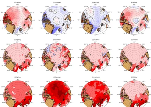
Figure 2 shows the seasonal mean differences of T2M, to-tal precipitation (TP) and snowfall (SF) between ERA5 and ERA-I over Arctic sea ice during 2010–2015. We classify spring as March, April and May, summer as June, July and August, autumn as September, October and November, and winter as December, January and February. The seasonal mean ice extent is obtained from the monthly sea ice con-centration from NOAA/NSIDC during 2010–2015 (Meier et al., 2017).

(4)

Arc-Figure 1.Drift trajectories of all selected buoys (IMBs and snow buoys) in 2010 to 2015. The symbol “?” indicates the start of the drift and “◦” signals the end of the drift. Buoys are labelled at the beginning or the end of the drift using the same colour as trajecto-ries. Buoys used for model simulations are highlighted with a solid thick line and bold font. Dashed thick lines illustrate our defini-tion for sectors: central Arctic (black; north of 86◦N), and south of 86◦N: Pacific sector (magenta; 90◦W–150◦E), Atlantic sector (cyan; 30◦W–60◦E) and Laptev Sea (orange; 60–150◦E) used in Fig. 6.

tic sea ice. These temperature differences are smaller dur-ing summer, but substantial durdur-ing the other seasons. Near the North Pole, ERA5 is warmer than ERA-I in summer, but colder than ERA-I in winter. Whether warmer or colder, the differences between ERA5 and ERA-I are small (±0.4◦C) in this region.

ERA-I is known to be a relatively “dry” global reanaly-sis product in the Arctic compared with most other modern reanalyses (e.g. MERRA-2, CFSR and JRA-55) (Lindsay et al., 2014; Merkouriadi et al., 2017; Boisvert et al., 2018). The TP in ERA5 is typically less than 10 mm water equiv-alent higher than for ERA-I in all seasons over Arctic sea ice, with the exception of the Atlantic sector in autumn, win-ter and spring where TP in ERA5 can be up to 30 mm wawin-ter equivalent larger (Fig. 2e, g, h). The patterns of seasonal TP over sea ice are very similar in ERA5 and ERA-I (Fig. S1 in the Supplement), and with the distinctly highest annual TP in the Atlantic sector (Fig. S2).

Snowfall is substantially higher in ERA5 than in ERA-I in all seasons (Fig. 2i–l), particularly in the Atlantic sec-tor, where SF is up to 50 mm snow water equivalent (SWE) higher in the spring, autumn and winter seasons (Fig. 2i–l). In summer snowfall is much larger in ERA5 in the central and eastern Arctic (30–50 mm SWE higher) (Fig. 2j). Thus

the differences in the snowfall between ERA5 and ERA-I are much larger than for TP in all seasons except winter (Fig. 2i– l vs. Fig. 2e–h; see also Fig. S2). The patterns of seasonal snowfall over sea ice are very similar in ERA5 and ERA-I (Fig. S1). Annual SF has increased all across the Arctic, more than TP, especially in the Atlantic sector (>100 mm) and eastern Arctic (Fig. S2).

3.2 Comparison of reanalysis near-surface

temperature, snowfall and precipitation against buoy observations

Both ERA-I and ERA5 accurately capture the observed evo-lution of MSLP measured by each of the buoys (not shown). The hourly difference between the reanalysis MSLP and ob-servations is no more than a few hectopascals. Excellent agreements between observed MSLP in the Arctic and earlier reanalyses have been shown in previous studies (e.g, Maksh-tas et al., 2007), demonstrating that MSLP is well simulated in reanalyses. In the following, we will focus on near-surface temperature, snowfall and total precipitation.

3.2.1 Evaluation of near-surface temperature in ERA5 and ERA-I using buoy observations

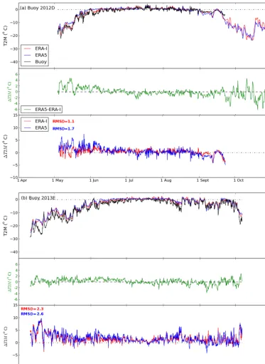
Figures 3–4 and S3–S5 show time series of T2M from differ-ent buoys, the corresponding T2M difference between ERA5 and ERA-I, and T2M differences between reanalyses and ob-servations at the buoys’ positions. The observed T2M reveals the pronounced seasonal cycle in the Arctic. Low tempera-tures persist through winter and spring, before approaching 0◦_{C in late May or early June. Temperatures near 0}◦_{C, or} oc-casionally over 0◦_{C, continue during summer, before lower} temperatures return in late August or early September and decrease further in autumn.

(5)

Figure 2.Seasonal mean difference between ERA5 and ERA-I (ERA5-ERA-I) for T2M(a–d), total precipitation(e–h)and snowfall(i–l)in spring(a, e, i), summer(b, f, j), autumn(c, g, k)and winter(d, h, l)over Arctic sea ice during 2010–2015.

Table 2.The mean T2M, accumulated FDD and estimated ice growth with the FDD model.

Buoy T2M mean (◦C) FDD (K d)a/ice growth (m)b

ERA5 ERA-I Buoy ERA5 ERA-I Buoy

2011M −22.5 −24.2 −26.6 4295/1.70 4662/1.78 5174/1.90 2012H −22.5 −24.1 −25.8 4276/1.70 4624/1.78 4978/1.85 2012L −22.1 −23.1 −24.9 4198/1.68 4402/1.73 4788/1.81

2012J −20.8 −20.8 NA 3902/1.61 3921/1.61 NA

NA: no data.a_{From 1 October to 30 April.}b_{Ice growth estimation by the end of freezing season with} the Lebedev FDD model (Maykut, 1986).

Graham et al., 2017b; Kayser et al., 2017; Biosvert et al., 2018). Interestingly, we find a larger warm bias in the new ERA5 compared with ERA-I (Figs. 3–4 and S3–S5, Table 2), despite the higher vertical resolution in ERA5. The root-mean-square deviation (RMSD) values are higher for ERA5 than for ERA-I (see Figs. 3–4 and S3–S5), in the range of 1.1–3.7◦C for ERA-I and 1.7–4.6◦C for ERA5.

We note that the near-surface air temperature in both re-analyses corresponds to a height of 2 m, while it is likely

(6)

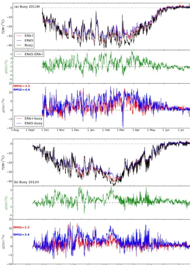
Figure 3. Variation in 2 m air temperature (T2M) in ERA5, ERA-I, and the buoys (upper panel) and the differences of T2M between ERA5 and ERA-I (mid-panel; green) and comparisons for ERA5 and ERA-I with buoys (ERA5 minus buoy; ERA-I minus buoy) for buoys (a)2012D and(b)2013E. RMSD values for the comparison between ERA products and buoys are shown as text, blue for ERA5-buoy, red for ERA-I-buoy.

ice were applied in both ERA5 and ERA-I. The misrepresen-tation of snow may affect the surface energy budget, physi-cally leading to, for example, overestimated conductive heat flux from the ocean to the surface.

(7)

Figure 4.Same as Fig. 3, but for(a)buoy 2011M and(b)buoy 2012H.

at air temperatures below −25◦C. The temperature depen-dence of the warm bias is also demonstrated in Fig. 5b, which shows the relationship between the daily mean T2M differ-ences with the temperature bins of 5◦C from−45 to+5◦C. When the T2M is below −25◦C, the daily mean difference between reanalysis and observation is higher than 2◦C, with ERA5 3.1–8.0◦C warmer than in buoys, and ERA-I 2.4–

4.4◦C warmer than in buoys (Fig. 5b). For air tempera-tures above−25◦C, the bias between reanalysis and buoys is smaller, with ERA5 and ERA-I both 0.75◦C warmer than the observations on average.

(8)

Figure 5.Statistics of T2M from ERA5, ERA-I and all the buoys.(a)Scatter plot for all data (small dots) and average T2M at 5◦bins between−45 and+5◦C,(b)daily temperature differences between the reanalysis and between the reanalysis and the buoys corresponding to 5◦bins between−45 and+5◦C, and(c)monthly mean differences and standard deviation (SD). In panel(a), the black solid line is for 1 : 1.

The smallest biases, and the smallest T2M differences be-tween ERA5 and ERA-I are found in the months bebe-tween July and October (also refer to Figs. 3–4 and S3–S5). ERA5 is typically warmer than ERA-I (and has a larger warm bias) throughout the winter and spring, including June. However, ERA5 is colder than ERA-I (0.01–0.6◦C) and has a smaller bias from July to October (Fig. 5c). Hence, the warm bias in ERA5 is smaller than ERA-I in the warm season (July– October). ERA-I has a warm bias in the warm season, but the magnitude is smaller (<0.8◦C) than the warm bias in the cold season (Fig. 5c). Similarly, ERA5 has a small warm bias during July and August (<1◦C), and a likely insignifi-cant cold bias (<0.2◦C) in September and October (Fig. 5c). The performance of reanalysis near-surface temperature varies with region over Arctic sea ice (Fig. 6; also refer to

(9)

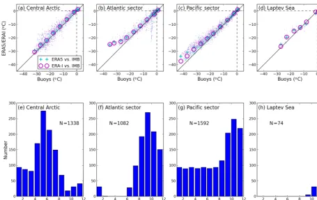
Figure 6.Scatter plot of T2M from ERA5 and ERA-I vs. from buoys for the(a)central Arctic,(b)Atlantic sector,(c)Pacific sector, and (d)Laptev Sea, and number of buoy data (daily) per month for the(e)central Arctic,(f)Atlantic sector,(g)Pacific sector, and(h)Laptev sea. The definition of sectors are shown in Fig. 1.

buoys are deployed in different regions of the Arctic and sub-sequent ice drift patterns.

3.2.2 Comparison of precipitation and snowfall from ERA5 and ERA-I along buoy drift trajectories We next compare the cumulative total precipitation and snowfall in ERA5 and ERA-I in autumn and winter, along the drift trajectories of the buoys. We begin accumulation from 15 August onwards if the buoy was deployed before this date, or from 1 October if the buoy was installed after 15 August but before 1 October. We accumulate the precipitation until 30 April, or until the buoy stopped working if this occurred before 30 April (Table 1).

The accumulated total precipitation (TP) in ERA5 is higher than ERA-I for all buoys (Figs. 7 and S6–S7, and Ta-ble 1), which is consistent with the seasonal difference in TP documented in Sect. 3.1 (Fig. 2e–h). On average, the accu-mulated TP in ERA5 is 13.8 mm water equivalent larger than in ERA-I, with differences for the individual buoys ranging from 0.4 (buoy 2013E; Fig. 7b) to 31.9 mm water equivalent (buoy 2012D; Fig. 7a). This is in agreement with the seasonal differences between the reanalyses (Fig. 2e–h).

Similar to the accumulated TP, the accumulated snowfall (SF) in ERA5 is larger than in ERA-I (Figs. 7 and S6–S7; Table 1). For buoys deployed near the North Pole that started

accumulating on 15 August, the accumulated SF in ERA5 is typically much larger than for ERA-I (Figs. 7a–b and S6, S7a). In contrast, for buoys deployed in other regions, which started accumulating on 1 October, the accumulated SF in ERA5 is typically slightly higher than ERA-I (Figs. 7c–d and S7b–f).

(10)

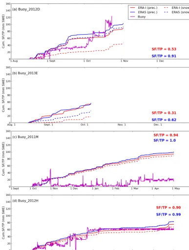
Arc-Figure 7.Cumulative total precipitation (TP) and snowfall (SF) for ERA5 and ERA-I and snow depth for buoys(a)2012D,(b)2013E, (c)2011M and(d)2012H. Accumulation starts from 15 August for panels(a)and(b)and from 1 October for panels(c)and(d). The ratio of snowfall to total precipitation (SF/TP) in ERA5 (blue text) and ERA-I (red text) is also shown in the figure. Note there were no snow depth data for buoy 2013E during the accumulation period.

tic sea ice (Fig. 8a–d vs. Fig. 8e–h). The increase in SF/TP ratio in ERA5 is more significant in autumn (∼0.2) and sum-mer (∼0.3–0.4) along the buoy trajectories, and relatively small in winter (∼0.1) and spring (∼0.1–0.2). This indi-cates more precipitation falls as snow in ERA5 not only in autumn but also in summer.

(11)

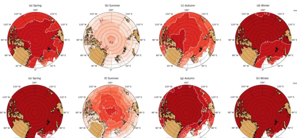
Figure 8.The ratio of snowfall to total precipitation (SF/TP) in ERA-I(a–d)and ERA5(e–h)in spring(a, e), summer(b, f), autumn(c, g) and winter(d, h).

only above 0◦C. In contrast, the IFS Cy41r2 used in ERA5 includes a prognostic microphysics scheme, with separate cloud liquid, cloud ice, rain and snow prognostic variables (Sotiropoulou et al., 2015; see also ECMWF IFS documen-tation – Cy41r2; https://www.ecmwf.int/sites/default/files/ elibrary/2016/16648-part-iv-physical-processes.pdf, last ac-cess: 4 March 2019). Our findings indicate that ERA5 has significantly less Arctic rainfall than ERA-I, particularly in autumn (Figs. 7, S6–S7) and summer (Fig. 8b and f).

Evaluating the performance of precipitation products over the Arctic Ocean is a major challenge due to the lack of observations, and difficulty accurately measuring snowfall (e.g. Lindsay et al., 2014; Rasmussen et al., 2012; Sato et al., 2017; Blanchard-Wrigglesworth et al., 2018; Boisvert et al., 2018; Webster et al., 2018). Here we compare the pre-cipitation from ERA-I and ERA5 with snow depth measure-ments from the buoys (Table 1). For this comparison, snow depth from the buoys is converted to snow water equivalent (SWE) using a climatological monthly mean snow density of 220–380 kg m−3(Warren et al., 1999). Caution must be taken here, as the buoys reflect point observations, while the re-analyses provide a grid cell average. Snow depth is known to have large variability even over relatively small spatial scales (Warren et al., 1999; Sturm et al., 2002; Liston et al., 2018). An unknown fraction of the true snowfall will also be lost through blowing snow into leads, which is not accounted for in our calculation.

The accumulated TP and SF from ERA-I and ERA5 are generally comparable with the observed SWE from buoys in most cases during the accumulation period (refer to Figs. 7 and S6–S7), such as for buoy 2012H deployed in the

Beau-fort Sea (Fig. 7d). However, in several cases the accumu-lated TP and SF from ERA-I and ERA5 are considerably lower than the observed SWE from buoys, such as for buoy 2012D from mid-September (Fig. 7a). This may be caused by snow drifting up against the buoy structure, or reflect anoma-lously low precipitation in the reanalyses. In other cases, the accumulated TP and SF from reanalysis is higher than the observed SWE from buoys during some periods [buoys 2013B (Fig. S6c) and s20 (Fig. S7e)] or for the whole ac-cumulation period [buoys 2011M (Fig. 7c), 2012L (Fig. 7c) and S29 (Fig. S7f)]. This could be caused by snow ero-sion/sublimation around the buoy, or reflect anomalously high precipitation in the reanalyses. By the end of the ac-cumulation period, the accumulated TP (SF) is larger on av-erage by 55.4 mm (41.9 mm) SWE for ERA-I and 66.5 mm (62.8 mm) SWE for ERA5 than the observed SWE of the snowpack along the buoy trajectories (see Table 1).

4 Influence of air temperature and precipitation on sea ice evolution during the freezing season

(12)

a complete freezing season (Table 1). These buoys were in-stalled on MYI or FYI in the central Arctic (buoy 2011M), the Beaufort Sea (buoy 2012H, buoy 2012L) or the Laptev Sea (buoy 2012J). When these buoys were installed, sea ice thickness was between 1 and 2 m for buoys 2011M, 2012H and 2012J, while buoy 2012L had an ice thickness of 3.35 m (Table 1). Snow depth was typically a few centimetres of snow at deployment. We use these buoys to assess the im-pact of different forcing data on sea ice evolution. For our simple approach we apply the empirical cumulative freezing degree day (FDD) model, which accounts for differences in T2M, and a 1-D sea ice model that also accounts for effects of precipitation and snowfall.

4.1 Assessing the sea ice evolution with freezing degree days (FDDs): impact of temperature bias

The cumulative freezing degree days (FDDs) model only needs air temperature as input and is often used to esti-mate sea ice growth (1h) from zero (e.g. Huntemann et al., 2014; Lei et al., 2017). The sea ice growth is estimated based on Lebedev (Maykut, 1986),1h=1.33P

(FDD)0.58, where

P

FDD is daily average temperature below the freezing point of sea water (−1.8◦C), integrated over the time period from 1 October to 30 April.

The positive near-surface air temperature bias in ERA5 and ERA-I results in a negative ice thickness bias at the end of the growth season. The cumulative FDD is smallest for ERA5 (Fig. S8, Table 2), corresponding to the largest warm bias in ERA5 during the freezing season. The differ-ences in FDD between ERA5, ERA-I and buoys are large for buoys 2011M, 2012H and 2012L, but negligible for buoy 2012J. The ice growth is 0.08–0.12 m less, with a mean of

−0.09 m for ERA-I T2M, and 0.13–0.20 m less, with a mean of −0.16 m for ERA5 T2M compared to when using near-surface buoy temperatures (Table 2).

4.2 Assessing sea ice evolution with a 1-D sea ice model HIGHTSI: impact of T2M and precipitation

HIGHTSI is a 1-D high-resolution thermodynamic snow and ice model designed for process studies to resolve the evolu-tion of snow–ice thickness and temperature profile. The snow and ice temperature regimes are solved by the partial dif-ferential heat conduction equations applied for snow and ice layers, respectively. The turbulent surface fluxes are param-eterized taking the thermal stratification of the atmosphere surface layer into account. Downward short- and longwave radiative fluxes are parameterized based on the total cloud cover. The model has been extensively used in Arctic studies (e.g. Cheng et al., 2008, 2013; Wang et al., 2015; Merkouri-adi et al., 2017).

In this section we perform six sensitivity simulations on each of the four buoys to explore the impact of temperature and precipitation on snow and sea ice evolution (Table 3).

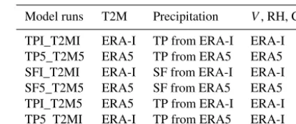
Table 3.Model runs and atmospheric forcing data in model simu-lations, where TP is total precipitation, SF is snowfall,V is wind at 10 m height, RH is relative humidity and CN is total cloud cover.

Model runs T2M Precipitation V, RH, CN

TPI_T2MI ERA-I TP from ERA-I ERA-I

TP5_T2M5 ERA5 TP from ERA5 ERA5

SFI_T2MI ERA-I SF from ERA-I ERA-I

SF5_T2M5 ERA5 SF from ERA5 ERA5

TPI_T2M5 ERA5 TP from ERA-I ERA-I TP5_T2MI ERA-I TP from ERA5 ERA-I

In the first two simulations, SFI_T2MI and SF5_T2M5, we force HIGHTSI with the T2M, 10 m wind speed (V), rel-ative humidity (RH), total cloud cover (CN) and snowfall, from ERA-I and ERA5 (Fig. S9), respectively. In the next two simulations, TPI_T2MI and TP5_T2M5, we force the model with the total precipitation from the reanalyses, rather than the snowfall, and treat precipitation as snow only when T2M is below 0◦C. In the final two simulations, we evaluate the influences of T2M and precipitation on the sea ice evo-lution individually. Specifically, we replace the T2M from ERA-I in the TPI_T2MI run with the T2M from ERA5, and name this run TPI_T2M5. Similarly, we replace the TP from ERA-I, in the run of TPI_T2MI, with the TP from ERA5 for the TP5_T2MI run (see Table 3). For all of the simula-tions we apply a seasonally variant ocean heat flux accord-ing to McPhee et al. (2003), which is large in October (10– 20 W m−2) and decreases to nearly zero from mid-November (see Fig. S9). Snow ice, an ice type formed at ice surface (e.g. Leppäranta, 1983), was recently found to significantly con-tribute to the Arctic sea ice mass balance in a region with thick snowpack on relatively thin ice (Granskog et al., 2017; Merkouriadi et al., 2017). A few (1.5–3) millimetres of snow ice formed only in the TPI_T2MI and TPI_T2M5 runs for buoy 2012J (with the lowest initial ice thickness of all buoys examined, Table 1). This is negligible for the total ice mass balance. Thus, the effect we examine solely depends on the differences in T2M and precipitation–snowfall on thermody-namic ice growth.

(13)

Figure 9.Evolution of snow and sea ice thickness during the freezing season based on simulations with HIGHTSI for(a)buoy 2012H, (b)buoy 2011M,(c)buoy 2012L and(d)buoy 2012J for runs TPI_T2MI, TP5_T2M5, SFI_T2MI and SF5_T2M5.

ice growth for buoy 2012H began in early December, at a rate of approximately 0.5 cm d−1, until late March, and af-terward the growth became sluggish at a rate of 0.16 cm d−1 until the end of April (Fig. 9a). However, buoy 2012L, which had an initial ice thickness of∼3.3 m, showed no significant growth until early February, before undergoing a slight in-crease from around 3.3 to 3.42 m by the end of the freezing

(14)

despite the larger warm bias in ERA5 (Fig. 9). Sea ice was marginally thinner (0.006–0.02 m) in TP5_T2M5 compared with TPI_T2MI for all the buoys. The major differences we see between these simulations is in the snow depth (Fig. 9). TPI_T2MI has a thinner snowpack than TP5_T2M5 for all four buoys, by 0.02–0.06 m. This is due to the higher total precipitation in ERA5, compared with ERA-I (see Sect. 3.2). In contrast, when HIGHTSI is forced with the reanaly-sis’ snowfall product (SFI_ERAI and SF5_ERA5) the dif-ferences in snow depth are comparable with the simu-lations forced by the total precipitation (TPI_T2MI and TP5_T2M5). The SFI_T2MI runs typically have a thinner snowpack (0.01–0.06 m) and a greater ice thickness (0.04– 0.09 m) than SF5_T2M5. The snow depth in SFI_T2MI is thinner (by 0.01–0.04 m) and ice thickness is greater (0.01– 0.06 m) than the TPI_T2MI runs (Fig. 9). This is because there is substantial rain at sub-zero temperatures in the SFI_T2MI runs that is classified as snow in the TPI_T2MI runs. There are no large differences between the snow depth and sea ice thickness at the end of the growth season for the SF5_T2M5 and TP5_T2M5 runs because, unlike in ERA-I, there is little rain at sub-zero temperatures for SF5_T2M5.

We now look at the effect of T2M differences between ERA5 and ERA-I, and compare the TPI_T2M5 runs vs. TPI_T2MI runs (Fig. 10). When using the T2M from ERA5 and not altering the precipitation forcing, the snowpack re-mains unchanged from the TPI_T2MI run. However, we find a slightly thinner ice at the end of the freezing season, com-pared with TPI_T2MI runs (0–0.04 m thinner), as a result of the larger warm bias in ERA5, which slows down the growth of sea ice. This is consistent with our results from the FDD model in Sect. 4.1.

Finally, we look at the effect of precipitation by compar-ing the TP5_T2MI and TPI_T2MI runs. The snowpack in TP5_T2MI is thicker (0.006–0.02 m), while the ice thick-ness is thinner (0.003–0.02 m) than in the TPI_T2MI runs (Fig. 10). The thicker snowpack is due to the higher precip-itation in ERA5 compared with ERA-I. This thicker snow-pack allows less heat loss to the atmosphere, which results in less ice growth.

Overall the difference of using different T2M and TP forc-ings is very moderate and equal in magnitude during the freezing period. Obviously using the ERA-I SF will result in larger differences, due to the low SF in ERA-I.

In general, HIGHTSI reproduces the evolution of snow and sea ice observed by the buoys well during the freez-ing season (Figs. 9–10) although there are some differences. For the snowpack, there was a 10 cm increase in snow depth for IMB_2012H during late December, which seems not well captured by any of the reanalyses and therefore by any of the simulations (Figs. 9a and 10a). The simulations for IMB_2012H show an increase in snow depth at the end of April, indicating a snowfall event in the reanalysis. However, this was not recorded by the buoy. Thus, not only the magni-tude but also the frequency of the precipitation in the

reanal-ysis data are crucial for the snow evolution in the simulation. The representation of snow in the model may further influ-ence the simulated ice thickness (e.g. Fig. 9a). Evaluating precipitation in the Arctic is however challenging as men-tioned previously due to the large local variability and lack of representative in situ observations (e.g. Liston et al., 2018). Differences in the modelled sea ice thickness from the buoy observations in part arise from not knowing the local ocean heat flux at each individual buoy; however, our approach is to look at the sensitivity relative to the differences in T2M and precipitation–snowfall in the reanalyses.

5 Conclusions

Atmospheric reanalysis are often used to force snow and sea ice models. The accuracy of these forcing products is paramount for the reproduction of the sea ice evolution in the model. ERA5 is a new global reanalysis product from ECMWF and will replace the widely used ERA-I. Here we compare the 2 m air temperature (T2M), snowfall, and total precipitation in ERA5 and ERA-I, and evaluate these prod-ucts against in situ observations from drifting buoys (IMBs and snow buoys) over Arctic sea ice.

Overall, we find a warm bias in ERA-I and ERA5, when compared with the buoys. In both reanalyses, the bias is smallest in summer months, and larger in autumn, winter and spring. The warm bias in ERA5 is smaller than ERA-I in summer. However, we find a larger warm bias in ERA5 than in ERA-I during the cold season, especially when the observed T2M was lower than−25◦C in the Atlantic sec-tor and Pacific secsec-tor. For days when the observed T2M was <−25◦_{C, the daily mean difference between the reanalyses} and buoys was, on average,+5.4◦C for ERA5 and+3.4◦C for ERA-I. The near-surface warm bias in ERA5 and ERA-I may partly be attributed to the difference in height with ob-servations. The larger warm bias in ERA5 during cold peri-ods suggests this reanalysis also struggles to accurately sim-ulate strong stable boundary layers, which frequently appear in winter and early spring, despite the higher vertical resolu-tion compared with ERA-I (e.g. Beesley et al., 2000).

(15)

Figure 10.Same as Fig. 9, but for model runs TPI_T2M5 and TP5_T2MI.

ERA-I is known to have an anomalously large fraction of liquid precipitation (rain) and thus low snowfall to precipita-tion ratio in the Arctic, especially during August–September (Dutra et al., 2011; Leeuw et al., 2015). The total precipi-tation accumulated along the buoy drift trajectories, during the cold season (from 15 August or 1 October until a buoy fails or until 30 April), was higher in ERA5 than in ERA-I for every buoy examined. The snowfall-to-precipitation ratio

(16)

snowpack, compared with the snowfall in ERA-I, which is often much less, suggesting the total precipitation and snow-fall in ERA5 are better represented. Nonetheless, the lack of representative in situ observations and difficulty in measuring snow accumulation on sea ice in the Arctic makes it a chal-lenge to accurately evaluate precipitation products over sea ice (e.g. Rasmussen et al., 2012; Lindsay et al., 2014; Sato et al., 2017; Blanchard-Wrigglesworth et al., 2018; Boisvert et al., 2018).

The larger warm bias during the ice growth season in ERA5, compared with ERA-I, can result in a lower ice thick-ness when using this as a forcing product for an ice model or a cumulative FDD model. The higher precipitation and snow-fall in ERA5 result in a thicker snowpack that allows less heat loss to the atmosphere. Overall, using a 1-D thermodynamic sea ice model simulation with ERA5 had a thinner ice thick-ness compared with ERA-I at the end of the growth season with a combined effect of higher T2M and more snow. How-ever, the effects on ice growth are very small (on the order of centimetres) during the freezing period. Given snow on sea ice is such a critical factor in sea ice evolution, more repre-sentative observations are therefore needed (e.g. Merkouriadi et al., 2017; Webster et al., 2018).

Data availability. IMB data are available at http:

//imb-crrel-dartmouth.org/archived-data/ (last access: 15 October 2017) and snow buoy data are available at http://www.meereisportal.de/en.html (last access: 17 January 2018)

Supplement. The supplement related to this article is available

online at: https://doi.org/10.5194/tc-13-1661-2019-supplement.

Author contributions. CW, KW and MAG initiated the study. CW

and MAG retrieved the buoy data. CW and KW downloaded and analysed the reanalysis data and performed the 1-D model simu-lations. All authors contributed to writing and to revisions of the paper.

Competing interests. The authors declare that they have no conflict

of interest.

Acknowledgements. The authors would like to thank Chris

Derk-sen, Alek Petty and the one anonymous reviewer, whose com-ments significantly improved this paper. We wish to acknowledge ECMWF for ERA-Interim and ERA5 data, the International Arctic Buoy Program (IABP) for the IMB data, and the Alfred Wegener Institute for Snow Buoy data.

Financial support. This research has been supported by the

Re-search Council of Norway (grant no. 254765), the Fram Centre “Arctic Ocean” flagship program through the SOLICE project, and by the Centre for Ice, Climate and Ecosystems (ICE) at the Norwe-gian Polar Institute through the N-ICE project.

Review statement. This paper was edited by Chris Derksen and

re-viewed by Alek Petty and one anonymous referee.

References

Albergel, C., Dutra, E., Munier, S., Calvet, J.-C., Munoz-Sabater, J., de Rosnay, P., and Balsamo, G.: ERA-5 and ERA-Interim driven ISBA land surface model simulations: which one performs better?, Hydrol. Earth Syst. Sci., 22, 3515–3532, https://doi.org/10.5194/hess-22-3515-2018, 2018.

Alexeev, V. A., Walsh, J. E., Ivanov, V. V., Semenov, V. A., and Smirnov, A. V.: Warming in the Nordic Seas, North Atlantic storms and thinning Arctic sea ice, Environ. Res. Lett., 12, 084011, https://doi.org/10.1088/1748-9326/aa7a1d, 2017. AMAP: Snow, Water, Ice and Permafrost in the Arctic (SWIPA)

2017. Arctic Monitoring and Assessment Programme (AMAP), Oslo, Norway, Xiv +269 pp, 2017.

Beesley, J. A., Bretherton, C. S., Jakob C., Anderas, E. L., In-trieri, J. M., and Uttal, T. A.: A comparison of cloud and boundary layer variables in the ECMWF forecast model with observations at Surface Heat Budget of the Arctic Ocean (SHEBA) ice camp, J. Geophys. Res., 105, 12337–12349, https://doi.org/10.1029/2000JD900079, 2000.

Bekryaev, R. V., Polyakov, I. V., and Alexeev, V. A.: Role of polar amplification in long-term surface air temperature varia-tions and modern arctic warming, J. Climate, 23, 3888–3906, https://doi.org/10.1175/2010JCLI3297.1, 2010.

Blanchard-Wrigglesworth, E., Webster, M. A., Farrell, S. L., and Bitz, C. M.: Reconstruction of snow on Arc-tic sea ice, J. Geophys. Res.-Oceans, 123, 3588–3602, https://doi.org/10.1002/2017JC013364, 2018.

Boisvert, L. N. and Stroeve, J. C.: The Arctic is becom-ing warmer and wetter as revealed by the Atmospheric Infrared Sounder, Geophys. Res. Lett., 42, 4439–4446, https://doi.org/10.1002/2015GL063775, 2015.

Boisvert, L. N., Webster, M. A.,Petty, A. A., Markus, T., Bromwich, D. H., and Cullather R. I.: Intercomparison of precipitation esti-mates over the Arctic Ocean and its peripheral seas from reanaly-ses, J. Climate, 31, 8441–8462, https://doi.org/10.1175/JCLI-D-18-0125.1, 2018.

Cheng, B., Zhang, Z., Vihma, T., Johansson, M., Bian, L., Li, Z., and Wu, H.: Model experiments on snow and ice thermodynamics in the Arctic Ocean with CHINARE 2003 data, J. Geophys. Res., 113, C09020, https://doi.org/10.1029/2007JC004654, 2008. Cheng, B., Mäkynen, M., Similä, M., Rontu, L., and Vihma,

T.: Modelling snow and ice thickness in the coastal Kara Sea, Russia Arctic, Ann. Glaciol., 54, 105–113, https://doi.org/10.3189/2013AoG62A180, 2013.

(17)

Dahlke, S. and Maturilli, M.: Contribution of Atmospheric Advection to the Amplified Winter Warming in the Arc-tic North AtlanArc-tic Region, Adv. Meteorol., 8, 4928620, https://doi.org/10.1155/2017/4928620, 2017.

Decker, M., Brunke, M. A., Wang, Z., Sakguchi, K., Zeng, X., and Bosilovich, M. G.: Evaluation of the reanalysis products from GSFC, NCEP, and ECMWF using flux tower observations, J. Climate, 25, 1916–1944, https://doi.org/10.1175/JCLI-D-11-00004.1, 2012.

Dee, D. P., Uppala, S. M., Simmons, A. J., Berrisford, P., Poli, P., Kobayashi, S., Andrae, U., Balmaseda, M. A., Balsamo, G., Bauer, P., Bechtold P., Beljaars, A. C. M., Berg, L. van de, Bid-lot, J., Bormann, N., Delsol, C., Dragani, R., Fuentes, M., Geer, A. J., Haimberger, L., Healy, S. B., Hersbach, H., Hólm, E. V., Isaksen, L., Kållberg, P., Köhler, M., Matricardi, M., McNally, A. P., Monge-Sanz, B. M., Morcrette, J.-J., Park, B.-K., Peubey, C., Rosany, P. de, Tavolato, C., Thépaut, J.-N., and Vitart, F.: The ERA-Interim reanalysis: configuration and performance of the data assimilation system, Q. J. Roy. Meteor. Soc., 137, 553–597, 2011.

Dutra, E., Schär, C., Viterbo, P., and Miranda, P. M. A.: Land-atmosphere coupling associated with snow cover, Geophys. Res. Lett., 38, L15707, https://doi.org/10.1029/2011GL048435, 2011. Graham, R. M., Cohen, L., Petty, A. A., Boisvert, L. N., Rinke, A., Hudson, S. R., Nicolaus, M., and Granskog, M. A.: Increasing frequency and duration of Arctic win-ter warming events, Geophys. Res. Lett., 44, 6974–6983, https://doi.org/10.1002/2017GL073395, 2017a.

Graham, R. M., Rinke, A., Cohen, L., Hudson, S. R., Walden, V. P., Granskog, M. A., Dorn, W., Kayser, M., and Maturilli, M.: A comparison of the two Arctic atmospheric winter states observed during N-ICE2015 and SHEBA, J. Geophys. Res.-Atmos., 122, 5716–5737, https://doi.org/10.1002/2016JD025475, 2017b. Granskog, M. A., Rösel, A., Dodd, P. A., Divine, D.,

Ger-land, S., Martma, T., and Leng, M. J.: Snow contribution to first-year and second-year Arctic sea ice mass balance north of Svalbard, J. Geophys. Res.-Oceans, 122, 2539–2549, https://doi.org/10.1002/2016JC012398, 2017.

Graversen, R. G., Mauritsen, T., Tjernström, M., Källén, E., and Svensson, G.: Vertical structure of recent Arctic warming, Na-ture, 451, 53–56, https://doi.org/10.1038/nature06502, 2008. Grosfeld, K. Treffeisen, R., Asseng, J., Bartsch, A., Bräuer, B.,

Fritzsch, B., Gerdes, R., Hendricks, S., Hiller, W., Heygster, G., Krumpen, T., Lemke, P., Melsheimer, C., Nicolaus, M., Ricker, R., and Weigelt, M.: Online sea-ice knowledge and data platform <www.meereisportal.de >, Polarforschung, Bre-merhaven, Alfred Wegener Institute for Polar and Marine Re-search and German Society of Polar ReRe-search, 85, 143–155, https://doi.org/10.2312/polfor.2016.011, 2016.

Hersbach, H. and Dee, D.: ERA5 reanalysis is in production, ECMWF Newsletter 147, ECMWF, available at: https://www. ecmwf.int/en/newsletter/147/news/era5-reanalysis-production (last access: 24 March 2017), 2016.

Huntemann, M., Heygster, G., Kaleschke, L., Krumpen, T., Mäkynen, M., and Drusch, M.: Empirical sea ice thick-ness retrieval during the freeze-up period from SMOS high incident angle observations, The Cryosphere, 8, 439–451, https://doi.org/10.5194/tc-8-439-2014, 2014.

Jakobson, E., Vihma, T., Palo, T., Jakobson, L., Keernik, H., and Jaagus, J.: Validation of atmospheric reanalyses over the central Arctic Ocean, Geophys. Res. Lett., 39, L10802, https://doi.org/10.1029/2012GL051591, 2012.

Kapsch, M. L., Graversen, R. G., Economou, T., and Tjernström, M.: The importance of spring atmospheric conditions for predic-tions of the Arctic summer sea ice extent, Geophys. Res. Lett., 41, 5288–5296, https://doi.org/10.1002/2014GL060826, 2014. Kayser, M., Maturilli, M., Graham, R. M., Hudson, S. R.,

Rinke, A., Cohen, L., Kim, J.-H., Park, S.-J., Moon, W., and Granskog, M. A.: Vertical thermodynamic structure of the tro-posphere during the Norwegian young sea ICE expedition (N-ICE2015), J. Geophys. Res.-Atmos., 122, 10855–10872, https://doi.org/10.1002/2016JD026089, 2017.

King, J., Spreen, G., Gerland, S., Haas, C., Hendriks, S., Kaleschke, L., and Wang, C.: Sea-ice thickness from field measurements in the northwestern Barents Sea, J. Geophys. Res.-Oceans, 122, 1497–1512, https://doi.org/10.1002/2016JC012199, 2017. Leeuw, J. D., Methven, J., and Blackburn, M.: Evaluation of

ERA-Interim reanalysis precipitation products using England and Wales observations, Q. J. Roy. Meteor. Soc., 141, 798–806, https://doi.org/10.1002/qj.2395, 2015.

Lei, R., Cheng, B., Heil, P., Vihma, T., Wang, J., Ji, Q., and Zhang, Z.: Seasonal and interannual variations of sea ice mass balance from the Central Arctic to the Greenland Sea, J. Geophys. Res.-Oceans, 123, 2422–2439, https://doi.org/10.1002/2017JC013548, 2017.

Leppäranta, M.: A growth model for black ice, snow ice and snow thickness in subarctic basins, Hydrol. Res., 14, 59–70, 1983. Lindsay, R. and Schweiger, A.: Arctic sea ice thickness loss

deter-mined using subsurface, aircraft, and satellite observations, The Cryosphere, 9, 269–283, https://doi.org/10.5194/tc-9-269-2015, 2015.

Lindsay, R., Wensnahan, M., Schweiger, A., and Zhang, J.: Eval-uation of seven different atmospheric reanalysis products in the Arctic, J. Climate, 27, 2588–2606, https://doi.org/10.1175/JCLI-D-13-00014.1, 2014.

Liston, G. E., Polashenski, C., Rösel, A., Itkin, P., King, J., Merk-ouriadi, I., and Haapala, J.: A distributed snow-evolution model for sea-ice applications (SnowModel), J. Geophys. Res.-Oceans, 123, 3786–3810, https://doi.org/10.1002/2017JC013706, 2018. Lüpkes, C., Vihma, T., Jakobson, E., König-Langlo, G.,

and Tetzlaff, A.: Meteorological observations from ship cruises during summer to the central Arctic: A compari-son with reanalysis data, Geophys. Res. Lett., 37, L09810, https://doi.org/10.1029/2010GL042724, 2010.

Makshtas, A., Atkinson, D., Kulakov, M., Shutilin, S., Krishfield, R., and Proshutinsky, A.: Atmospheric forcing validation for modeling the central Arctic, Geophys. Res. Lett., 34, L20706, https://doi.org/10.1029/2007GL031378, 2007.

Maksimovich, E. and Vihma, T.: The effect of surface heat fluxes on interannual variability in the spring onset of snow melt in the central Arctic Ocean, J. Geophys. Res., 117, C07012, https://doi.org/10.1029/2011JC007220, 2012.

(18)

Maslanik, J., Stroeve, J., Fowler, C., and Emery, W.: Distribution and trends in Arctic sea ice age through spring 2011, Geophys. Res. Lett., 38, L13502, https://doi.org/10.1029/2011GL047735, 2011.

Maykut, G. A.: The surface heat and mass balance, in: Geophysics of Sea Ice, edited by: Untersteiner, N., Plenum, New York, USA, 395–463, 1986.

McPhee, M. G., Kikuchi, T., Morison, J. H., and Stan-ton, T. P.: Ocean-to-ice heat flux at the North Pole En-vironmental observatory, Geophys. Res. Lett., 30, 2274, https://doi.org/10.1029/2003GL018580, 2003.

Meier, W. N., Fetterer, F., Savoie, M., Mallory, S., Duerr, R., and Stroeve, J.: NOAA/NSIDC climate data record of pas-sive microwave sea ice concentration, Version 3. Boulder, Col-orado USA, NSIDC, National Snow and Ice Data Center, https://doi.org/10.7265/N59p2ZTG, 2017.

Merkouriadi, I., Cheng, B., Graham, R. M., Rösel, A., and Granskog, M. A.: Critical Role of Snow on Sea Ice Growth in the Atlantic Sector of the Arctic Ocean, Geophys. Res. Lett., 44, 10479–10485, https://doi.org/10.1002/2017GL075494, 2017. Mortin, J., Graversen, R. G., and Svensson, G.: Evaluation of

pan-Arctic melt-freeze onset in CMIP5 climate models and reanal-yses using surface observations, Clim. Dynam., 42, 2239–2257, https://doi.org/10.1007/s00382-013-1811-z, 2014.

Mortin, J., Svensson, G., Graversen, R. G., Kapsch, M. L., Stroeve, J. C., and Boisvert, L. N.: Melt onset over Arctic sea ice con-trolled by atmospheric moisture transport, Geophys. Res. Lett., 43, 6636–6642, https://doi.org/10.1002/2016GL069330, 2016. Nicolaus, M., Hoppmann, M., Arndt, S., Hendricks, S., Kaltein,

C., König-Langlo, G., Nicolaus, A., Rossmann, L., Schiller, M., Schwegmann, S., Langevin, D., and Bartsch, A.: Snow height and air temperature on sea ice from snow buoy measurements, Alfred Wegener Institute, Helmholtz Center for Polar and Marine Research, Bremerhaven, PANGAEA, https://doi.org/10.1594/PANGAEA.875638, 2017.

Olauson, J.: ERA5: The new champion of wind power modelling? Renew. Energ., 126, 322–331, https://doi.org/10.1016/j.renene.2018.03.056, 2018.

Perovich, D., Richter-Menge, J., and Polashenski, C.: Observing and understanding climate changes: Monitoring the mass bal-ance, motion, and thickness of Arctic sea ice, available at: http: //imb-crrel-dartmouth.org/, last access: 15 October 2017. Polashenski, C., Perovich, D., Richter-Menge, J., and Elder, B.:

Seasonal ice mass-balance buoys: adapting tools to the changing Arctic, Ann. Glaciol., 52, 18–26, 2011.

Rasmussen, R., Baker, B., Kochendorfer, J., Meyers, T., Landolt, S., Fischer, A. P., Black, J., Thériault, J. M., Kucera, P., Gochis, D., Smith, C., Nitu, R., Hall, M., Ikeda, K., and Gutmann, E.: How well are we measuring snow: The NOAA/FAA/NCAR win-ter precipitation test bed, B. Am. Meteorol. Soc., 93, 811–829, https://doi.org/10.1175/BAMS-D-11-00052.1, 2012.

Richter-Menge, J., Perovich, D. K., Elder, B. C., Claffey, K., Rigor, I., and Ortmeyer M.: Ice mass balance buoys: a tool for measur-ing and attributmeasur-ing changes in the thickness of the Arctic sea ice cover, Ann. Glaciol., 44, 205–210, 2006.

Rigor, I. G., Colony, R. L., and Martin, S.: Variations in Surface Air Temperature Observations in the Arctic, 1979–97, J. Climate, 13, 896–914, 2000.

Rinke, A., Maturilli, M., Graham, R. M., Matthes, H., Handorf, D., Cohen, L., Hudson, S. R., and Moore J. C.: Extreme cy-clone events in the Arctic: Wintertime variability and trends, Environ. Res. Lett., 12, 094006, https://doi.org/10.1088/1748-9326/aa7def, 2017.

Sato, K. and Inoue, J.: Comparison of Arctic sea ice thickness and snow depth estimates from CFSR with in situ observations, Clim. Dynam., 50, 1–13, https://doi.org/10.1007/s00382-017-3607-z, 2017.

Schweiger, A., Lindsay, R., Zhang, J., Steele, M., Stern, H., and Kwok, R.: Uncertainty in modeled Arctic sea ice volume, J. Geophys. Res.-Oceans, 116, 1–21, https://doi.org/10.1029/2011JC007084, 2011.

Screen, J. A. and Simmonds, I.: The central role of diminishing sea ice in recent Arctic temperature amplification, Nature, 464, 1334–1337, https://doi.org/10.1038/nature09051, 2010. Sotiropoulou, G., Sedlar, J., Forbes, R., and Tjernström, M.:

Sum-mer Arctic clouds in the ECMWF forecast model: An evaluation of cloud parameterization schemes, Q. J. Roy. Meteor. Soc., 142, 387–400, https://doi.org/10.1002/qj.2658, 2015.

Stroeve, J. and Notz D.: Chaning state of Arctic sea ice across all the seasons, Environ. Res. Lett., 13, 103001, https://doi.org/10.1088/1748-9326/aade56, 2018.

Stroeve, J. C., Serreze, M. C., Holland, M. M., Kay, J. E., Malanik, J., and Barrett A. P.: The Arctic’s rapidly shrinking sea ice cover: A research synthesis, Climatic Change, 110, 1005–1027, https://doi.org/10.1007/s10584-011-0101-1, 2012.

Stroeve, J. C., Markus, T., Boisvert, L., Miller, J., and Bar-rett, A.: Changes in Arctic melt season and implications for sea ice loss, Geophys. Res. Lett., 41, 1216–1225, https://doi.org/10.1002/2013GL058951, 2014.

Stroeve, J. C., Schroder, D., Tsamados, M., and Feltham, D.: Warm winter, thin ice?, The Cryosphere, 12, 1791–1809, https://doi.org/10.5194/tc-12-1791-2018, 2018.

Sturm, M., Holmgren, J., and Perovich, D. K.: Winter snow cover on the sea ice of the Arctic Ocean at the Surface Heat Budget of the Arctic Ocean (SHEBA): Temporal evo-lution and spatial variability, J. Geophys. Res., 107, 8047, https://doi.org/10.1029/2000JC000400, 2002.

Tjernstöm, M. and Graversen, R. G: The Vertical Structure of the lower Arctic troposphere analysed from observations and the ERA-40 reanalysis, Q. J. Roy. Meteor. Soc., 135, 431–443, https://doi.org/10.1002/qj.380, 2009.

Urraca, R., Huld, T., Gracia-Amillo, A., Martinez-de-Pison, F. J., Kaspar, F., and Sanz-Garcia, A.: Evaluation of global horizontal irradiance estimates from ERA5 and COSMO-REA6 reanalysis using ground and satellite-based data, Sol. Energy, 164, 339–354, https://doi.org/10.1016/j.solener.2018.02.059, 2018.

Vihma, T., Pirazzini, R., Fer, I., Renfrew, I. A., Sedlar, J., Tjern-ström, M., Lüpkes, C., Nygård, T., Notz, D., Weiss, J., Marsan, D., Cheng, B., Birnbaum, G., Gerland, S., Chechin, D., and Gascard, J. C.: Advances in understanding and parameteriza-tion of small-scale physical processes in the marine Arctic cli-mate system: a review, Atmos. Chem. Phys., 14, 9403–9450, https://doi.org/10.5194/acp-14-9403-2014, 2014.

(19)

ice mass-balance buoy (IMB) data, Ann. Glaciol., 54, 253–260, https://doi.org/10.3189/2013AoG62A135, 2013.

Wang, C., Cheng, B., Wang, K., Gerland, S., and Pavlova O.: Modelling snow ice and superimposed ice on landfast sea ice in Kongsfjorden, Svalbard, Polar Res., 34, 20828, https://doi.org/10.3402/polar.v34.20828, 2015.

Warren, S. G., Rigor, I. G., Untersteiner, N., Radionov, V. F., Bryaz-gin, N. N., Aleksandrov, Y. I., and Colony, R.: Snow depth on Arctic sea ice, J. Climate, 12, 1814–1829, 1999.

Webster, M., Gerland, S., Holland, M., Hunke, E., Kwok, R., Lecomte, O., Massom, R., Perovich, D., and Sturm, M.: Snow in the changing sea-ice systems, Nat. Clim. Change, 8, 946–953, https://doi.org/10.1038/s41558-018-0286-7, 2018.

Wesslén, C., Tjernström, M., Bromwich, D. H., de Boer, G., Ek-man, A. M. L., Bai, L.-S., and Wang, S.-H.: The Arctic summer atmosphere: an evaluation of reanalyses using ASCOS data, At-mos. Chem. Phys., 14, 2605–2624, https://doi.org/10.5194/acp-14-2605-2014, 2014.