Alexander Schaaf and Clare E. Bond
Department of Geology and Petroleum Geology, School of Geosciences, University of Aberdeen, AB24 3UE, Aberdeen, UK Correspondence:Alexander Schaaf ([email protected])
Received: 14 March 2019 – Discussion started: 2 April 2019
Revised: 10 June 2019 – Accepted: 12 June 2019 – Published: 5 July 2019
Abstract. In recent years, uncertainty has been widely rec-ognized in geosciences, leading to an increased need for its quantification. Predicting the subsurface is an especially un-certain effort, as our information either comes from spatially highly limited direct (1-D boreholes) or indirect 2-D and 3-D sources (e.g., seismic). And while uncertainty in seismic in-terpretation has been explored in 2-D, we currently lack both qualitative and quantitative understanding of how interpre-tational uncertainties of 3-D datasets are distributed. In this work, we analyze 78 seismic interpretations done by final-year undergraduate (BSc) students of a 3-D seismic dataset from the Gullfaks field located in the northern North Sea. The students used Petrel to interpret multiple (interlinked) faults and to pick the Base Cretaceous Unconformity and Top Ness horizon (part of the Middle Jurassic Brent Group). We have developed open-source Python tools to explore and visualize the spatial uncertainty of the students’ fault stick interpreta-tions, the subsequent variation in fault plane orientation and the uncertainty in fault network topology. The Top Ness hori-zon picks were used to analyze fault offset variations across the dataset and interpretations, with implications for fault throw. We investigate how this interpretational uncertainty interlinks with seismic data quality and the possible use of seismic data quality attributes as a proxy for interpretational uncertainty. Our work provides a first quantification of fault and horizon uncertainties in 3-D seismic interpretation, pro-viding valuable insights into the influence of seismic image quality on 3-D interpretation, with implications for determin-istic and stochastic geomodeling and machine learning.
1 Introduction
Geosciences, and geology in particular, are concerned with integrating various sources of data, often of limited, sparse and indirect nature, into scientific models. The use of lim-ited data combined with our limlim-ited knowledge of the highly complex Earth system invariably infuses any model with un-certainty, especially as geology inherently relies heavily on interpreted data that often require reasoning about processes that occur over geological timescales (Frodeman, 1995), which further increase the space of uncertainty.
Thore et al., 2002; Thiele et al., 2016; Godefroy et al., 2018). Additionally, the process of interpretation between seismic lines and cubes is fundamentally different and thus might lead to conceptually different uncertainties to be dominant (e.g., the need to connect fault evidence between seismic lines introduces significant uncertainty in widely spaced 2-D interpretation compared to fault interpretation in seismic cubes; see Freeman et al., 1990).
In this work, we investigate the scope of uncertainties in 3-D seismic interpretation. We qualitatively and quantitatively analyze interpretations of 78 final-year undergraduate (BSc) students conducted on a 3-D seismic cube of the Gullfaks field. The dataset depicts a comparatively simple geometry of planar domino-style normal faults, but the seismic dataset exhibits high amounts of noise, especially in its eastern half, and generally increasing with depth and in fault proximity (see Fig. 8a, b). This inhibits straightforward interpretation of major faults and horizons and limits use of structural seismic attributes. We analyze the spatial variation in fault stick inter-pretations and the subsequent uncertainty in fault orientation. Horizon interpretations are analyzed and combined with fault interpretations for a description of fault throw uncertainty. Additionally, we investigate the differences in fault network topology (see Morley and Nixon, 2016; Peacock et al., 2016, 2017) in the interpretation ensemble to better estimate the un-certainty of interpreting fault networks in 3-D seismic data. We use the interpretation of Fossen and Hesthammer (1998) as a reference expert example (in the sense of Macrae et al., 2016) to compare fault network topology and fault orienta-tion uncertainty with the student interpretaorienta-tions. We integrate our findings of interpretation uncertainties with its relation to seismic data quality and discuss the implications for both de-terministic and stochastic geomodeling, as well as machine learning applied to seismic interpretation.
2 Materials and methods
2.1 Gullfaks geology and seismic data
We give here a brief overview over the regional and struc-tural geology of the study area; a more in-depth description of the structural geology of the Gullfaks field can be found in Fossen and Hesthammer (1998).
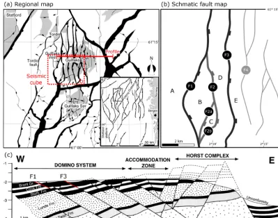
The Gullfaks field is a subset of the NNE–SSW-trending, 10–25 km wide Gullfaks fault block, located in the western part of the Viking Graben within the northern North Sea (see Fig. 1a). The Gullfaks field’s reservoir units reach from the late Triassic Hegre Group, over the Early Jurassic Statfjord Formation, Dunlin Group up to the Brent Group (Hestham-mer and Fossen, 1997). The reservoir units are separated from the Upper Cretaceous sediments above by the Base Cre-taceous Unconformity (Fossen and Hesthammer, 1998). The field consists of three structurally distinct domains: a struc-turally simple domino system in the western part and the
structurally more complex accommodation zone and Horst complex towards the east (see Fig. 1c). Our study focuses on the structurally simpler western part of the domino system, where we investigate the uncertainty of the three faults (F1– F3) and the fault blocks (A–E) depicted in Fig. 1b. Note that Faults 1 and 2 merge in the northern half and at the bottom of the domain and that Fault 2 splits into two smaller faults (F2a and F2b).
The 3-D seismic survey of the Gullfaks field, ST85R9211, was recorded in 1985 and reprocessed in 1992. It was recorded in time and converted to depth using two-way travel time (TWT) depth conversion and was migrated using a pre-stack Kirchhoff migration.
2.2 Interpretation dataset
The analyzed interpretations were produced as part of the Surface and Subsurface Digital Imaging course within the undergraduate Geology and Petroleum Geology program at the University of Aberdeen. While the students had prior training in structural geology and interpretation of 2-D seis-mic data, this was the students’ first hands-on course in 3-D seismic interpretation using the Petrel software as part of their undergraduate program. The fourth-year undergraduate (BSc) students loaded the seismic data into Petrel together with 14 wells, while ensuring proper georeferencing. The fol-lowing interpretation process focused on first interpreting the Top Cretaceous horizon with initial support by the lecturing staff. Afterwards, the students started to independently inter-pret the Base Cretaceous Unconformity (BCU) and Top Ness horizon (which is part of the Brent Group) around well loca-tions, followed by connecting the horizon interpretation in between wells. The students were instructed to mainly use guided auto-tracking, as well as occasional seeded tracking and manual interpretation where possible or necessary, de-pending on seismic data quality. Afterwards, fault interpre-tations were conducted of major faults. The students then interpolated surfaces from the horizon interpretations using Petrel’smake surfacefunction. Polygons were created based on fault locations to create a Top Ness surface subdivided into the fault blocks.
Figure 1. (a)Regional overview of the Gullfaks–Statfjord area located in the northern North Sea, showing the location of the Gullfaks oil field.(b)Fault map of the Statfjord Formation, showing the main faults of the Gullfaks field and their labeling.(c)Cross-section across the Gullfaks field, depicting the three distinct structural domains, major faults and stratigraphy (modified from Fossen and Hesthammer, 1998).
Figure 2. Example interpretation from a single student, showing the three major faults considered in our study as well as part of the Top Ness horizon interpretation. Base Cretaceous Unconformity (BCU) and additional faults towards the east are hidden for better visualization of the key elements.
2.3 Data analysis
To process and analyze the large amount of interpretation data, the exported Petrel surfaces and fault sticks were wran-gled using custom Python functionality and labeled in an open tabular data format. The result is a set of 4 460 878 data points, belonging to 78 student interpretations, with 228 unique faults considered, which consist of a total 10 052 individual fault sticks. For data processing and analysis, we made heavy use of the open-source Python packages pan-das, SciPy and NumPy (McKinney, 2011; Jones et al., 2001; Oliphant, 2006).
extensively in between students. The resulting normal vector can be converted into strike and dip values. For visualization, the fault orientation data were subdivided into three regu-lar bins oriented E–W across the structures. The fault throw analysis is based on the Top Ness horizon and is computed individually at each interpreted fault stick for each fault and each interpretation. The fault throw for each interpretation is then averaged into 20 bins along theyaxis to make the anal-ysis independent of the number of fault sticks interpreted by each student. The nearest data points on both the hangingwall and footwall of the Ness horizon fault blocks were selected as seeds. From these seeds, the surface data approximately or-thogonal to strike were used within a strike-parallel window of three grid cells (approximately 570 m). A relative gradient filter was then used to exclude points with gradients to their nearest neighbors outside of the interquartile range (IQR) of the selected subset. The resulting data are fitted with a linear regression for each fault block and the intersection with the fault stick used to calculate fault throw.
Throughout this work, we make use of the term “seismic data quality” not in the strictly geophysical sense of quality factors surrounding seismic data acquisition and processing but rather in the sense of the interpretability of the seismic data. If the seismic data lack clear, continuous reflectors in a region but show a noisy image difficult to interpret – no matter what the source of this may be – we describe them as an area of low seismic data quality. Similarly, if reflector strengths are high and continuous (for horizon interpretation) or clearly offset (for fault interpretation), we speak of high seismic data quality.
For the assessment of seismic reflector strength, an rms amplitude seismic attribute (RMSA for short) was calculated using Petrel’s rms amplitude function using a window length of 24 traces. The rms amplitude represents the square root of the arithmetic mean of squared amplitude values across a specified seismic trace window.
3 Results
3.1 Uncertainty in fault interpretation
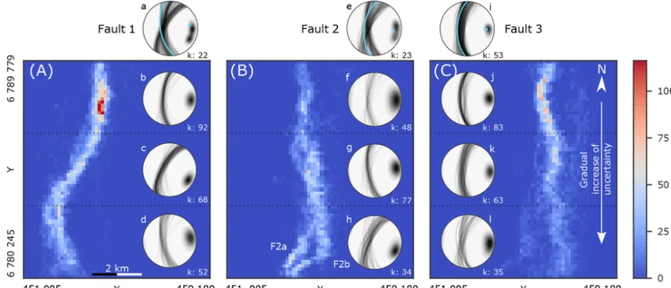
Figure 3 shows 2-D histograms for the three major faults taken into consideration within this study. The histograms cover the entire extent of the seismic cube, with the fre-quency of fault stick points counted per bin in a depth slice at 2 km±0.1. Fault 1 shows a sigmoidal shape in the N–S direction of the seismic depth slice (see Fig. 3A), with high-frequency densities in the northern part and lower intensities found in the southern part. Plotting all fault plane orienta-tions within a single stereonet reveals three distinct clusters of planes (Fig. 3a), which when separated into three equal bins along the N–S axis correspond to the components of the sigmoidal fault shape (Fig. 3b–d). We have added Bingham mean poles from Fossen and Hesthammer (1998) for all three
faults in the plot (light blue) for comparison. Interpretations of Fault 2 show a split into two sub-faults (F2a and F2b) in the southern part (see Fig. 3B), as also interpreted by Fos-sen and Hesthammer (1998, see Fig. 1). The spatial uncer-tainty of the fault interpretations appears slightly lower in the northern part of the seismic slice but also shows evidence of a small separated fault block in the central part of the fault. The interpretations of Fault 3 show a strong increase in dispersion towards the southern part of the seismic slice (Fig. 3C). The same trend of increasing uncertainty can be observed in the fault plane orientation (Fig. 3j–l). Additionally, the histogram shows the occasional interpretation of the fault branching to-wards Fault 2b, toto-wards the west, and toto-wards Fault 4 to the east (see Fig. 1b). The effect of fault stick interpreta-tion frequency between the students with below-median and above-median fault stick interpretation frequency on overall fault standard deviation was analyzed using Bayesian esti-mation for two groups (Kruschke, 2013). We observed dif-ferences in mean standard deviation of 35.8, 20.2 and 81.5 m for Faults 1, 2 and 3, respectively, with probability of the differences being larger than zero being 99.3 %, 87.4 % and 99.9 %, respectively, making the differences for Faults 1 and 3 statistically credible.
Figure 3 plots fault plane orientations calculated from stu-dents’ fault stick interpretations. Fault 1 shows three distinct clusters of orientations (Fig. 3A, a–d), which can be sepa-rated by subdividing the study domain into three equal bins along the N–S axis. Fault 1 shows a striking decrease ink val-ues (a measure of tightness of the orientation clusters) from north to south (92, 68, 52). The pattern does not hold true for Fault 2, which shows lowkvalues both in the north and south. Fault 3 shows similar behavior to Fault 1, with a strong increase in dispersion from north to south (83, 63, 35).
Overall, the observed uncertainty (standard deviation) of the fault plane along the W–E axis appears to be increas-ing linearly with depth for all three faults (Fig. 4). Note that the overall mean standard deviations between the faults vary greatly: 791, 384 and 575 m for Faults 1, 2 and 3, respec-tively. The extremely high variation of standard deviations seen in the upper part of Fig. 4 (faded data points) is due to a few students extending their fault interpretations above the BCU, making the data points at that depth statistically un-reliable due to low sample numbers and geologically ques-tionable. Any fault stick interpretations above the BCU were thus excluded from the least-squares linear regression (R val-ues for Faults 1, 2 and 3: 0.75, 0.85 and 0.61).
Figure 3.2-D histograms for Faults 1(A), 2(B)and 3(C)for the depth slice at 2 km±0.1. Stereonet plots of Faults 1–3 (columns) with all fault strike orientations along the fault length plotted combined in the first row(a, e, i). To discriminate changing trends in actual fault orientation from interpretation uncertainty, rows two to four plot data from bins separated by dashed blue lines, from the northern(c, g, k), middle(d, g, l)and southern bins(e, h, m). Blue planes and poles in the top row(a, e, i)show Bingham analysis mean pole from Fossen and Hesthammer (1998) for reference.
Figure 4.Scatter plot of mean (collapsedyaxis) standard deviation alongxaxis of mean fault surfaces for Faults 1, 2 and 3. Chaotic patterns of uncertainty at shallow depths (faded data points) are likely due to sporadic numbers of interpretations, as students often stopped interpreting the faults before reaching the BCU. Overall, uncertainty of fault interpretations is increasing linearly with depth (linear regression only takes into account interpretations below the BCU;R values for Faults 1, 2 and 3, respectively: 0.75, 0.85 and 0.61).
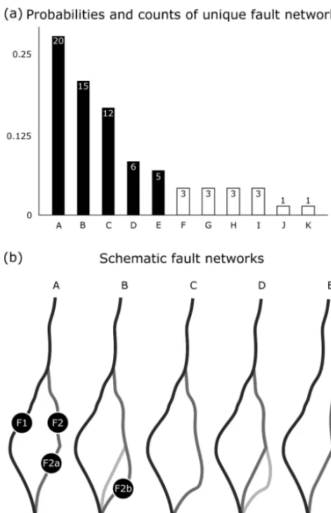
expert FN interpretation of Fossen and Hesthammer (1998), which corresponds to either the second or fourth most com-mon FN interpretations (Fig. 5b, B and D). The major source of uncertainty in this specific FN appears to be interpreting both F2a and F2b, and which one abuts the other. The few students who branched off the southern part of Fault 3 to-wards the west interpreted Fault 2b as part of Fault 3 but did not connect it to the FN of Faults 1 and 2.
3.2 Fault throw and horizon uncertainties
Figure 5.Probabilities of unique fault network topologies(a)with corresponding schematic fault networks(b)of the five most likely networks.
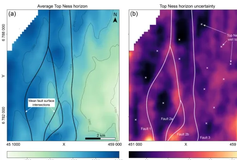
Figure 7a shows the average Top Ness horizon basemap for all interpretations combined. Overall, the horizon inter-pretations are increasing in depth from SE towards the NW of the domain. Figure 7b shows the associated standard devia-tion of the average Ness horizon interpretadevia-tion, with an over-lay of mean fault intersections and well locations. We ob-serve large horizon uncertainties in proximity to both Faults 1 and 2 throughout the dataset. An increase of horizon un-certainty occurs at the southern end of the domain where Faults 1 and 2 begin to merge again. In the north, the hori-zon uncertainty surrounding Fault 3 decreases rapidly with distance from the fault, with two well tops and packages of high reflector strength (see Fig. 8A) constraining the un-certainty. As the seismic data quality decreases towards the south (see Fig. 8B), the uncertainty in the horizon interpreta-tion increases in the eastern part of the dataset. Interpretainterpreta-tion uncertainties are significantly reduced surrounding well loca-tions in the western part of the study domain, where seismic reflectors of the Top Ness horizon are overall stronger and
more continuous (see Fig. 8A). This pattern does not hold true in the east of the dataset, where reflector continuity is overall low and noise in the seismic dataset is high.
3.3 Seismic data quality
To assess influences of seismic data quality on fault inter-pretation uncertainty, we made use of the RMSA attribute as a proxy for reflector strength (strong horizon reflectors aiding the interpretation of faults result in high RMSA val-ues). Specifically, we investigated the example of Fault 3, as it shows significant gradual changes in interpretation uncer-tainty across the seismic dataset (Figs. 3C and 6b). Figure 8 shows four averaged RMSA responses with corresponding fault stick interpretation histograms (Fig. 8a–d) from the lo-cations shown as white boxes in Fig. 8.1. In the northern ex-tent of the seismic slice, Fault 3 is closely bounded by strong horizon reflectors, as shown in the RMSA slice (Fig. 8.1), seismic slice (Fig. 8.2) and inline section A, focusing the stu-dents’ interpretations, as seen in the corresponding histogram of fault interpretations (Fig. 8a). The histogram shows a bi-modal distribution, as some students interpreted the fault fur-ther towards the east, where anofur-ther fault is present (Fault 4; see Fig. 1b). The overall uncertainty related to the interpreta-tion of the actual Fault 3 is approximately normal distributed (skewness of 0.33), with the width of the trough seen in the RMSA response containing more than±1.8 standard devia-tions (92.8 %) of the fault stick placement uncertainty. Fur-ther towards the south of the dataset, the RMSA response diminishes east of Fault 3, while remaining strong on the western side (Fig. 8b). The fault interpretations show a 64 % increase in standard deviation, with thicker tails in the his-togram (79 % increase of Pearson kurtosis), especially to-wards the west, where interpretations are then bounded by strong seismic reflectors. Further south, the seismic response degrades and is noisy (Fig. 8.1 and B), leading also to a lack of signal in the RMSA values (Fig. 8c). The corre-sponding fault stick placements increase in uncertainty (in-crease in standard deviation by 289 %), now appearing nearly uniformly distributed with a slight crest (Fig. 8c). At the southern end of the slice, RMSA responses increase again (Fig. 8d). The distribution of fault interpretations shows a bi-modal distribution, as seen before in the map-view 2-D his-tograms shown in Fig. 3.
4 Discussion 4.1 Key findings
Figure 6.Results of fault throw analysis for Faults 1(a)and 3(b)visualized as box plots, showing median fault throw (black lines) with interquartile range (grey boxes), minima and maxima whiskers (grey lines) and outliers (grey dots).
Figure 7. (a)Basemap of average Top Ness horizon from all interpretations;(b)standard deviation of the average Top Ness horizon from all interpretations with overlaid mean fault surfaces (white lines) and well-top locations (white crosses).
near-maximal uncertainty in areas of low seismic image data quality (Fig. 8c). The spread in fault stick placement appears to not be entirely driven by seismic noise but rather appears to be, at least partly, guided by the surrounding interpreta-tions in areas of higher data quality (Fig. 8b, d), allowing
Our study also shows that uncertainties in the placement of faults sticks appear to increase linearly with depth (Fig. 4). This is an important finding for approximating uncertainty trends with depth and is especially important as seismic im-age quality tends to decrease with depth.
Our analysis of Top Ness horizon interpretation uncertain-ties shows the correlation of uncertainty with fault proximity (Fig. 7b). Horizon interpretations surrounding Fault 3 in the northern part show only slight increases in uncertainty to-wards the fault, as they are strongly constrained by wells and high reflector continuity (see Figs. 7b and 8A). With decreas-ing seismic data quality towards the south, we also see an in-crease in uncertainty surrounding Fault 3, which also shows in the increasing fault throw uncertainty seen in Fig. 6b. This trend is not as evident for the throw across Fault 1, with the Top Ness horizon being better constrained on both sides, with overall higher seismic image data quality. Qualitative com-parison of median fault throw for both Fault 1 and Fault 2 with depth maps in Fossen and Hesthammer (1998) display-ing fault heave can be made under the simplifydisplay-ing assump-tion of constant fault dip. Fault heave qualitatively mimics the patterns we found in our uncertainty study: gradual de-crease from north to south for Fault 3 and the stark differ-ences where Faults 1 and 2 merge, as well as the increase towards the south. This comparison consolidates the confi-dence in our automated fault throw analysis and hints at the validity of aggregating a large number of interpretations of even non-experts to assess geological features.
We have also shown uncertainty in fault orientations (Fig. 3) and the inadequacy of summarizing fault orientation using a deterministic mean pole, as in Fossen and Hestham-mer (1998), who calculated it using Bingham analysis of data from a different 3-D seismic dataset. This inadequacy results from sinusoidal fault map pattern (Fig. 3A) and curved 3-D geometries on top of uncertain fault stick placements.
We observed strong decreases in uncertainty surrounding wells in the west of the study area (Fig. 7b). The trend of increasing uncertainty in horizon location from west to east could be attributed to the decrease in seismic image data quality and thus the much lower reflector continuity. But we would also expect for the horizon uncertainties to be reduced
uncertainty. We have quantified the impact of fault tainty on fault network topology and fault and horizon uncer-tainty on fault throw. The fault network topology in a “tradi-tional” deterministic geomodel is important, as it determines the number of fault blocks and hence the degree to which stratigraphic units are separated (by faults). This informa-tion is imperative to the understanding of reservoir compart-mentalization in hydrocarbon reservoirs, connectivity and flow characteristics of groundwater aquifers and useful for geothermal projects. Simply, reservoir performance can be significantly affected by fault network topology, and under-standing these uncertainties, and hence reservoir connectiv-ity, can be critical to the planning of production strategies (e.g., Manzocchi et al., 2008a, b; Lescoffit and Townsend, 2005; Tveranger et al., 2008). The type of fault network topology information available in Fig. 5 could be used to in-form reservoir modeling to guide multiple production strate-gies (e.g., multiple deterministic models are made) and for informed history matching during field operation when reser-voir models have been developed from single deterministic models and need to be updated.
transfer (e.g., to inform nuclear waste disposal engineering) or hydrocarbon and energy production.
4.3 Implications for stochastic modeling
Although we can outline how uncertainty information could be used to better inform use of deterministic models and their inherent uncertainties, advances in both computational ca-pabilities and implicit structural geomodeling have allowed for major improvements in the incorporation of uncertain-ties into structural geomodels by means of stochastic simula-tions. At its core, stochastic structural geomodeling requires adequate disturbance distributions to obtain reasonable es-timates of geomodel uncertainty (see Wellmann and Cau-mon, 2018). This uncertainty parameterization can be used to better establish and account for interpretation uncertainties on top of deterministic modeling workflows using a hybrid approach based on a single deterministic or multiple deter-ministic models: for example, a deterdeter-ministic fault network topology model with fault throw uncertainties parameterized or multiple deterministic models to characterize the most probable fault network topologies (e.g., Fig. 5) with fault throw uncertainties parameterized. Such hybrid approaches may provide the best solutions when the time and computa-tional costs of full stochastic modeling are too high and/or when elements of the uncertainty in the geomodel are not best represented as simple stochastic functions, such as dif-ferent conceptual models (e.g., for fault network topologies). Stamm et al. (2019) have recently explored how both fault throw and fault sealing uncertainty can be incorporated into stochastic geological modeling workflows, and studies like ours can help inform stochastic parameterization with how fault throw uncertainties can change along strike depending on changes in the seismic data quality.
The work of Pakyuz-Charrier et al. (2018) discusses the importance of proper parameterization of input data mea-surement uncertainty when constructing stochastic geomod-els, but little is known about the uncertainties in interpreting the dense 3-D seismic datasets to obtain such input data for structural geomodels. Our work not only provides a first look at how significant these uncertainties can be but additionally provides a first-order approximation for parameterization of fault and horizon interpretation uncertainties within stochas-tic geomodels based on seismic image quality surrounding fault interpretations. Future research into how our findings could be integrated with the seismic expression of fault zones (e.g., Botter et al., 2014; Iacopini et al., 2016) could fur-ther our ability to parameterize stochastic geomodels directly from seismic data.
While student interpretations will most certainly reside within the upper range of interpretation uncertainty, we argue that they nevertheless provide significant value to stochas-tic parameterization, especially to the emergent Bayesian ap-proaches to stochastic structural geomodeling (Caers, 2011; de la Varga and Wellmann, 2016; Wellmann et al., 2017), as
they could provide informed – but not overly constrained – prior parameterization that can be reduced by case-specific geological likelihood functions and auxiliary data integra-tion. We also agree with Caers (2018) on the need for a rig-orous methodology of falsification in geomodeling. The in-tegration of adequately parameterized seismic interpretation uncertainties into a Bayesian geomodeling framework could enable a quality control of the interpretation by probabilis-tic assessment of the stochasprobabilis-tic geomodel against geologi-cal likelihood functions (e.g., fault length and throw relation-ships, fault population distributions, analog studies).
Our findings underline the complexity involved in the adequate parameterization of interpretation uncertainty in stochastic geomodeling: while normal distributions may cap-ture uncertainty adequately in areas of good seismic imag-ing (Fig. 8a), skewed fat-tailed distributions (e.g., Cauchy; Fig. 8b) or even uniform distributions (Fig. 8c) are reason-able choices with degrading seismic quality. When implic-itly modeling 3-D geological surfaces, many approaches are based on both surface points and strike and dip informa-tion. The latter carry significantly higher amounts of infor-mation (Calcagno et al., 2008; Laurent et al., 2016; Grose et al., 2017) than the surface points, thus emphasizing the need to quantify their uncertainty if it is used to generate and constrain 3-D stochastic geomodels. The use of von Mises– Fisher distributions to model uncertainty of orientation vec-tors was shown as a robust way to describe surface orienta-tion uncertainty (Pakyuz-Charrier et al., 2018), and our anal-ysis could provide valuable information for their parameteri-zation in areas of high interpretation uncertainty within sed-imentary basins.
4.4 Implications for machine learning
perturbations of the same to let NNs learn how ideal struc-tures that underlie noisy seismic image data might look like. They could then possibly generate possible higher-quality re-alizations of noisy, uncertain areas of seismic images to sup-port interpretation efforts. Overall, the complex interplay of the underlying geology, computational and conceptual chal-lenges of the machine learning approaches and the human-induced uncertainties will require strongly interdisciplinary approaches to combine state-of-the-art algorithms and geo-logical domain knowledge to further automate the laborious and uncertain task of 3-D seismic interpretation.
5 Summary
Our study provides a first look and quantification of the scale of uncertainties involved in the structural interpretation of data-dense 3-D seismic data. We have found the following:
– Fault placement uncertainty shows strong dependency on seismic data quality. The use of a seismic attribute (rms amplitude) showed promising first results to be used as a proxy for estimating fault interpretation un-certainties. This can be especially valuable for the pa-rameterization of stochastic geomodels based on single seismic reference interpretations.
– The common use of normal distributions as pertur-bance distributions in stochastic geomodeling seems in-adequate in areas where interpretation uncertainty is high (low seismic data quality). Instead, uncertainty pa-rameterization should always be directly linked to the surrounding seismic data quality and the use of near-uniform distributions can be recommended in areas of extremely poor interpretability.
– We found that relative trends of fault placement un-certainty can be approximated linearly with depth, al-though we recommend more research to further investi-gate the influence of seismic data quality in combination with changes in reflector continuity with depth.
or techniques used and training background in an attempt to consider the influence of these factors on the statistical distri-butions of interpretation outcome. Such factors may also vary depending on different tectonic and stratigraphic settings, so inclusion of a range of geological contexts may also be im-portant. Together, such uncertainties could be integrated into future geomodeling efforts and decision making, as well as informing training, workflows and expertise development.
Code availability. The Python libraryuninterpwas written to pro-vide convenient functionality for the wrangling of exported Petrel interpretation data and uncertainty analysis of multiple interpre-tations. It is a free, open-source library licensed under the GNU Lesser General Public License v3.0 (GPLv3.0). It is hosted as a git repository (https://github.com/pytzcarraldo/uninterp) on GitHub (Schaaf, 2019; https://doi.org/10.5281/zenodo.2593587).
Author contributions. Both AS and CEB conceptualized the re-search and were responsible for project administration, rere-search val-idation and writing, reviewing and editing the manuscript. CEB was also responsible for project supervision and funding acquisition. AS was responsible for data curation, formal analysis, methodology de-velopment, software development and data visualization.
Competing interests. The authors declare that they have no conflict of interest.
Disclaimer. This research was conducted within the scope of a To-tal GRC-funded postgraduate research project.
Special issue statement. This article is part of the special issue “Understanding the unknowns: the impact of uncertainty in the geo-sciences”. It is not associated with a conference.
pro-viding extensive information about the interpretation process and helpful input during the data analysis. Special thanks go to both Billy Andrews and Awad Bilal for their detailed reviews that helped us to significantly improve the manuscript of this work.
Financial support. Alexander Schaaf was supported by Total GRC UK research funding, with Clare E. Bond supported by a Royal Society of Edinburgh research sabbatical grant.
Review statement. This paper was edited by Lucia Perez-Diaz and reviewed by Billy Andrews and Awad Bilal.
References
Abrahamsen, P., Lia, O., and Omre, H.: An Integrated Ap-proach to Prediction of Hydrocarbon in Place and Recov-erable Reserve With Uncertainty Measures, in: European Petroleum Computer Conference, Society of Petroleum Engi-neers, https://doi.org/10.2118/24276-MS, 1992.
Alcalde, J., Bond, C. E., Johnson, G., Butler, R. W., Cooper, M. A., and Ellis, J. F.: The Importance of Structural Model Avail-ability on Seismic Interpretation, J. Struct. Geol., 97, 161–171, https://doi.org/10.1016/j.jsg.2017.03.003, 2017a.
Alcalde, J., Bond, C. E., Johnson, G., Ellis, J. F., and Butler, R. W.: Impact of Seismic Image Quality on Fault Interpretation Uncertainty, GSA Today, 27, 4–10, https://doi.org/10.1130/GSATG282A.1, 2017b.
Alcalde, J., Bond, C. E., and Randle, C. H.: Framing Bias: The Ef-fect of Figure Presentation on Seismic Interpretation, Interpreta-tion, 5, T591–T605, 2017c.
Biondi, B.: 3D Seismic Imaging, Investigations in Geophysics, Society of Exploration Geophysicists, Tulsa, Oklahoma, USA, https://doi.org/10.1190/1.9781560801689, 2006.
Bond, C., Gibbs, A., Shipton, Z., and Jones, S.: What Do You Think This Is? “Conceptual Uncertainty” in Geoscience Interpreta-tion, GSA Today, 17, 4, https://doi.org/10.1130/GSAT01711A.1, 2007.
Bond, C. E.: Uncertainty in Structural Interpretation: Lessons to Be Learnt, J. Struct. Geol., 74, 185–200, https://doi.org/10.1016/j.jsg.2015.03.003, 2015.
Bond, C. E., Philo, C., and Shipton, Z. K.: When There Isn’t a Right Answer: Interpretation and Reasoning, Key Skills for Twenty-First Century Geoscience, Int. J. Sci. Educ., 33, 629– 652, https://doi.org/10.1080/09500691003660364, 2011. Botter, C., Cardozo, N., Hardy, S., Lecomte, I., and Escalona,
A.: From Mechanical Modeling to Seismic Imaging of Faults: A Synthetic Workflow to Study the Impact of Faults on Seismic, Mar. Petrol. Geol., 57, 187–207, https://doi.org/10.1016/j.marpetgeo.2014.05.013, 2014. Caers, J.: Modeling Uncertainty in the Earth
Sci-ences: Caers/Modeling Uncertainty in the Earth Sci-ences, John Wiley & Sons, Ltd, Chichester, UK, https://doi.org/10.1002/9781119995920, 2011.
Caers, J.: Bayesianism in the Geosciences, in: Handbook of Mathematical Geosciences: Fifty Years of IAMG, edited by: Daya Sagar, B., Cheng, Q., and Agterberg,
F., pp. 527–566, Springer International Publishing, Cham, https://doi.org/10.1007/978-3-319-78999-6_27, 2018.
Calcagno, P., Chilès, J. P., Courrioux, G., and Guillen, A.: Geo-logical Modelling from Field Data and GeoGeo-logical Knowledge: Part I. Modelling Method Coupling 3D Potential-Field Interpola-tion and Geological Rules, Phys. Earth Planet. In., 171, 147–157, https://doi.org/10.1016/j.pepi.2008.06.013, 2008.
de la Varga, M. and Wellmann, J. F.: Structural Geologic Modeling as an Inference Problem: A Bayesian Perspective, Interpretation, 4, SM1–SM16, https://doi.org/10.1190/INT-2015-0188.1, 2016. Dramsch, J. and Lüthje, M.: Deep-Learning Seismic Facies on State-of-the-Art CNN Architectures, in: SEG Technical Program Expanded Abstracts 2018, SEG Technical Program Expanded Abstracts, pp. 2036–2040, Society of Exploration Geophysicists, Tulsa, Oklahoma, USA, https://doi.org/10.1190/segam2018-2996783.1, 2018.
Fossen, H. and Hesthammer, J.: Structural Geology of the Gullfaks Field, Northern North Sea, Geological Society, London, Special Publications, 127, 231–261, https://doi.org/10.1144/GSL.SP.1998.127.01.16, 1998.
Freeman, B., Yielding, G., and Badley, M.: Fault Correlation during Seismic Interpretation, First Break, 8, 87–95, 1990.
Frodeman, R.: Geological Reasoning: Geology as an In-terpretive and Historical Science, Geol. Soc. Am. Bull., 107, 960–0968, https://doi.org/10.1130/0016-7606(1995)107<0960:GRGAAI>2.3.CO;2, 1995.
Godefroy, G., Laurent, G., and Bonneau, F.: Structural Interpreta-tion of Sparse Fault Data Using Graph Theory and Geological Rules, Mathematical Geosciences, 1–17, published online, 2018. Grose, L., Laurent, G., Aillères, L., Armit, R., Jessell, M., and Caumon, G.: Structural Data Constraints for Im-plicit Modeling of Folds, J. Struct. Geol., 104, 80–92, https://doi.org/10.1016/j.jsg.2017.09.013, 2017.
Hesthammer, J. and Fossen, H.: Seismic Attribute Analysis in Struc-tural Interpretation of the Gullfaks Field, Northern North Sea, Petrol. Geosci., 3, 13–26, 1997.
Hu, Z., Ma, X., Liu, Z., Hovy, E., and Xing, E.: Harnessing Deep Neural Networks with Logic Rules, arXiv:1603.06318 [cs, stat], 2016.
Huang, L., Dong, X., and Clee, T. E.: A Scalable Deep Learning Platform for Identifying Geologic Features from Seismic Attributes, The Leading Edge, 36, 249–256, https://doi.org/10.1190/tle36030249.1, 2017.
Iacopini, D., Butler, R., Purves, S., McArdle, N., and De Fres-lon, N.: Exploring the Seismic Expression of Fault Zones in 3D Seismic Volumes, J. Struct. Geol., 89, 54–73, https://doi.org/10.1016/j.jsg.2016.05.005, 2016.
Jones, E., Oliphant, E., Peterson, P., et al.: SciPy: Open Source Sci-entific Tools for Python, available at: http://www.scipy.org/ (last access: 3 July 2019), 2001.
Kruschke, J. K.: Bayesian Estimation Supersedes the t Test, J. Exp. Psychol. Gen., 142, 573–603, https://doi.org/10.1037/a0029146, 2013.
Laurent, G., Ailleres, L., Grose, L., Caumon, G., Jessell, M., and Armit, R.: Implicit Modeling of Folds and Over-printing Deformation, Earth Planet. Sc. Lett., 456, 26–38, https://doi.org/10.1016/j.epsl.2016.09.040, 2016.
reser-K. D., Howell, J. A., Matthews, J. D., Walsh, J. J., Nepveu, M., Bos, C., Cole, J., Egberts, P., Flint, S., Hern, C., Holden, L., Hovland, H., Jackson, H., Kolbjørnsen, O., MacDonald, A., Nell, P. a. R., Onyeagoro, K., Strand, J., Syversveen, A. R., Tchistiakov, A., Yang, C., Yielding, G., and Zimmer-man, R. W.: Sensitivity of the Impact of Geological Uncertainty on Production from Faulted and Unfaulted Shallow-Marine Oil Reservoirs: Objectives and Methods, Petrol. Geosci., 14, 3–15, https://doi.org/10.1144/1354-079307-790, 2008a.
Manzocchi, T., Matthews, J. D., Strand, J. A., Carter, J. N., Skorstad, A., Howell, J. A., Stephen, K. D., and Walsh, J. J.: A Study of the Structural Controls on Oil Recovery from Shallow-Marine Reservoirs, Petrol. Geosci., 14, 55–70, https://doi.org/10.1144/1354-079307-786, 2008b.
McKinney, W.: pandas: a foundational Python library for data anal-ysis and statistics, Python for High Performance and Scientific Computing, 14, 1–9, 2011.
Morley, C. K. and Nixon, C. W.: Topological Characteristics of Sim-ple and ComSim-plex Normal Fault Networks, J. Struct. Geol., 84, 68–84, https://doi.org/10.1016/j.jsg.2016.01.005, 2016. Oliphant, T. E.: A Guide to NumPy, vol. 1, Trelgol Publishing USA,
2006.
Pakyuz-Charrier, E., Lindsay, M., Ogarko, V., Giraud, J., and Jes-sell, M.: Monte Carlo simulation for uncertainty estimation on structural data in implicit 3-D geological modeling, a guide for disturbance distribution selection and parameterization, Solid Earth, 9, 385–402, https://doi.org/10.5194/se-9-385-2018, 2018. Peacock, D., Nixon, C., Rotevatn, A., Sanderson, D., and Zu-luaga, L.: Interacting Faults, J. Struct. Geol., 97, 1–22, https://doi.org/10.1016/j.jsg.2017.02.008, 2017.
Peacock, D. C. P., Nixon, C. W., Rotevatn, A., Sander-son, D. J., and Zuluaga, L. F.: Glossary of Fault and Other Fracture Networks, J. Struct. Geol., 92, 12–29, https://doi.org/10.1016/j.jsg.2016.09.008, 2016.
Schaaf, A.: pytzcarraldo/uninterp: Paper: Quantification of uncer-tainty in 3-D seismic interpretation (Version paper_SE), Zenodo, https://doi.org/10.5281/zenodo.2593587, 2019.
https://doi.org/10.1190/1.1484528, 2002.
Tveranger, J., Howell, J., Aanonsen, S. I., Kolbjørnsen, O., Semshaug, S. L., Skorstad, A., and Ottesen, S.: Assessing Struc-tural Controls on Reservoir Performance in Different Strati-graphic Settings, Geological Society, London, Special Publica-tions, 309, 51–66, https://doi.org/10.1144/SP309.4, 2008. Tversky, A. and Kahneman, D.: Availability: A Heuristic for
Judg-ing Frequency and Probability, Cognitive Psychol., 5, 207–232, https://doi.org/10.1016/0010-0285(73)90033-9, 1973.
Tversky, A. and Kahneman, D.: Judgment under Uncer-tainty: Heuristics and Biases, Science, 185, 1124–1131, https://doi.org/10.1126/science.185.4157.1124, 1974.
Vrolijk, P. J., Urai, J. L., and Kettermann, M.: Clay Smear: Review of Mechanisms and Applications, J. Struct. Geol., 86, 95–152, https://doi.org/10.1016/j.jsg.2015.09.006, 2016.
Wellmann, J. F. and Caumon, G.: 3-D Structural Geological Mod-els: Concepts, Methods, and Uncertainties, in: Advances in Geo-physics, Elsevier, Cambridge, USA, San Diego, USA, Oxford, UK, London, UK, vol. 59, 1st edn., 2018.
Wellmann, J. F., de la Varga, M., Murdie, R. E., Gessner, K., and Jessell, M.: Uncertainty Estimation for a Geological Model of the Sandstone Greenstone Belt, Western Australia – Insights from Integrated Geological and Geophysical Inversion in a Bayesian Inference Framework, Geological Society, London, Special Pub-lications, p. SP453.12, https://doi.org/10.1144/SP453.12, 2017. Wu, X., Shi, Y., Fomel, S., and Liang, L.: Convolutional
Neu-ral Networks for Fault Interpretation in Seismic Images, in: SEG Technical Program Expanded Abstracts 2018, SEG Tech-nical Program Expanded Abstracts, pp. 1946–1950, Society of Exploration Geophysicists, https://doi.org/10.1190/segam2018-2995341.1, 2018.