The Cryosphere, 8, 1639–1650, 2014 www.the-cryosphere.net/8/1639/2014/ doi:10.5194/tc-8-1639-2014
© Author(s) 2014. CC Attribution 3.0 License.
A sea ice concentration estimation algorithm utilizing
radiometer and SAR data
J. Karvonen
Finnish Meteorological Institute (FMI), Helsinki, PB 503, 00101, Finland
Correspondence to: J. Karvonen ([email protected])
Received: 7 March 2014 – Published in The Cryosphere Discuss.: 28 April 2014 Revised: 24 July 2014 – Accepted: 29 July 2014 – Published: 5 September 2014
Abstract. We have studied the possibility of combining the high-resolution synthetic aperture radar (SAR) segmenta-tion and ice concentrasegmenta-tion estimated by radiometer bright-ness temperatures. Here we present an algorithm for map-ping a radiometer-based concentration value for each SAR segment. The concentrations are estimated by a multi-layer perceptron (MLP) neural network which has the AMSR-2 (Advanced Microwave Scanning Radiometer 2) polarization ratios and gradient ratios of four radiometer channels as its inputs. The results have been compared numerically to the gridded Finnish Meteorological Institute (FMI) ice chart con-centrations and high-resolution AMSR-2 ASI (ARTIST Sea Ice) algorithm concentrations provided by the University of Hamburg and also visually to the AMSR-2 bootstrap algo-rithm concentrations, which are given in much coarser res-olution. The differences when compared to FMI daily ice charts were on average small. When compared to ASI ice concentrations, the differences were a bit larger, but still small on average. According to our comparisons, the largest differences typically occur near the ice edge and sea–land boundary. The main advantage of combining radiometer-based ice concentration estimation and SAR segmentation seems to be a more precise estimation of the boundaries of different ice concentration zones.
1 Introduction
Ice concentration is defined as the ratio of the ice-covered area to the total area for a given sea region. From this def-inition, it directly follows that ice concentration is depen-dent on the resolution of the measurement. This fact also complicates direct comparison to different ice concentration
1640 J. Karvonen: A sea ice concentration estimation algorithm
cover, have not yet been widely used in measuring sea ice concentration. Some studies using single-band SAR for the estimation of ice concentration have however been made, e.g. those reported in Bovith and Andersen (2005), Berg (2011), Karvonen (2012) and Karvonen et al. (2012). Automated sea ice classification schemes, which implicitly include ice con-centration or an open-water class, based on single-band and dual-band SAR texture and backscattering, have also been proposed, e.g. in Clausi and Jernigan (2000), Clausi (2001), Deng and Clausi (2004, 2005), Maillard et al. (2005), Yu and Clausi (2007), Ochilov and Clausi (2012) and Leigh et al. (2014). These methods use multiple techniques, like the grey-level co-occurrence texture features (Haralick at al., 1973), Markov random fields (MRF) (Rue and Held, 2005), and Gabor filters (Pichler et al., 1996; Clausi and Jernigan, 2000) for classifying the sea ice SAR data. Dokken et al. (2000) developed a SAR ice concentration algorithm which is a combination of mean ratio (relating average SAR backscatter to typical open-water and sea ice values), a local threshold and a wavelet method (to detect edges around ice floes) for RADARSAT-1 (the first satellite of a series of Canadian earth observation satellites with a C-band SAR instrument) and ERS (European Remote Sens-ing satellite of the European Space Agency) SAR imagery. It has also been shown that using dual-polarized C-band SAR data (HH/HV) improves the ice concentration esti-mation compared to single-channel SAR (HH) (Karvonen, 2014). A method for ice classification into four ice classes and open water by combining SSM/I (Special Sensor Mi-crowave/Imager) radiometer ice concentration and SAR data was introduced in Kaleschke and Kern (2000). Here we pro-pose a novel method combining high-resolution SAR im-age segmentation and the lower-resolution radiometer ice concentration estimation to yield ice concentration estimates with improved areal boundaries defined by the SAR resolu-tion. The algorithm is based on SAR image segmentation and on multi-layer perceptron (MLP) neural network.
2 Study area, time and data
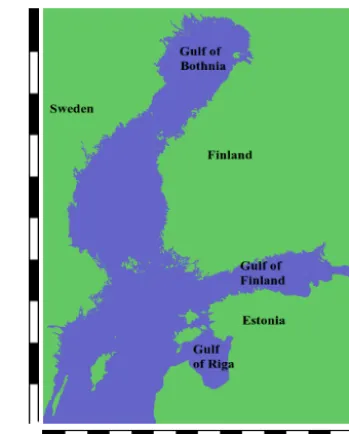
We studied our novel algorithm for the Baltic Sea. The study area is defined by the upper left and lower right corner in Fig. 1 (56.0◦N, 16.0◦E and 66.0◦N, 31.0◦E, respectively). The area of the Baltic Sea is 422 000 km2. Baltic Sea ice cover has large annual and local variations. Annual max-imum ice extent varies between 52 000 and 422 000 km2, the average being 218 000 km2(reached in January–March). The Bay of Bothnia and Gulf of Finland have at least par-tial ice cover every year. Baltic Sea ice moves and the ice concentration changes during each winter; also, some melt-ing can occur even in midwinter because the temperature may also vary from −40 to +10◦C even during midwin-ter. Only the landfast ice areas covering a relatively narrow zone along the coasts (from a few kilometres to a few tens of
Discussion
P
ap
er
|
Discussion
P
ap
er
|
Discussion
P
ap
er
|
Di
scuss
ion
P
ap
er
|
Fig. 1.The Baltic Sea study area. In the image scales the interval is one degree in both latitude and
longitude, the upper left corner is (66oN,16oE) and lower right corner (56oN,31oE).
figure
27
Figure 1. The Baltic Sea study area. In the image scales the interval
is 1◦in both latitude and longitude; the upper left corner is located at
66◦N, 16◦E, and the lower right corner is located at 56◦N, 31◦E.
kilometres) remain stable and typically have a high concen-tration throughout the winter. Winter 2013–2014 was a mild ice winter in the Baltic, and the air temperature also varied from cold to warm (above zero) many times during the win-ter.
The radiometer data were AMSR-2 radiometer level 1R brightness temperature data (Maeda, 2013). The SAR data were dual-polarized (HH/HV polarization combination) RADARSAT-2 ScanSAR Wide mode data. In this study we only utilized the HH channel of the SAR data. The SAR mo-saics were georectified to Mercator projection, and an inci-dence angle correction was applied to each SAR image in-cluded in the mosaic. The ice concentration estimates were also produced in Mercator projection, mapped and resam-pled to the resolution of 500 m, which corresponds to the projection and resolution of our SAR mosaics. In the projec-tion, we used the WGS84 datum, and the reference latitude (true scale latitude) was 61◦400N. The data set was divided into a training data set, consisting of daily SAR mosaics and AMSR-2 brightness temperature mosaics from 23 January to 1 February 2014, and a test data set, consisting of daily SAR mosaics and the corresponding daily AMSR-2 bright-ness temperature mosaics from 2 to 11 February 2014. Both data sets included 10 SAR mosaics and the corresponding daily AMSR-2 brightness temperature images.
J. Karvonen: A sea ice concentration estimation algorithm 1641
period varied; there was a short cold period (1–2 days), then a warmer period and then colder again. During the test pe-riod, there were two warmer periods and one colder period (not as cold as the one short cold period during the training period with the lowest temperature of−17◦C). There were also cases of wet snow over the sea ice and dry snow over the sea ice during both the training and the test period.
We also performed tests for two of our test area image mo-saics in the Kara and Barents seas. In this Arctic test area the projection was polar stereographic with the WGS84 da-tum. The mid-longitude was 55◦E and the true-scale latitude 70◦N. The latitudes in the area range from about 65 to 85◦N and longitudes from 0 to 90◦E. The ice and weather condi-tions in this Arctic area are different from the Baltic Sea. Typ-ically the weather during the winter months is colder, usually clearly below 0◦C, and the snow cover is typically wet only during the melting period starting in May–June. Also, in this Arctic test area, the ice concentrations vary because the ice is moving in most parts of the Arctic test area. Due to the colder temperatures less ice melting occurs during wintertime. In the Baltic, it is typical that some areas melt and refreeze dur-ing the wintertime due to rapid temperature changes.
3 Ice concentration estimation algorithm 3.1 SAR Processing
The SAR images were processed according to our standard procedure: first, they were calibrated and rectified to Mer-cator projection; then an incidence angle correction was ap-plied according to Makynen et al. (2002). After this, daily SAR mosaics were computed by remapping the SAR im-ages onto the study area such that newer data were always overlaid over older data, producing mosaics with the newest SAR data in each mosaic grid cell or pixel. The resolution of the SAR mosaics was 500 m. After this a segmentation step was performed for the daily mosaic. Here we have used an MRF-based segmentation adapted from Kato et al. (1992) and Berthod et al. (1996), but in practice any feasible seg-mentation, such as ICM (iterated conditional modes) (Besag, 1986) or even K means (MacQueen, 1967), can be used with rather similar results. The SAR segments smaller than 100 pixels (corresponding to an area of 25 km2) were com-bined with the adjacent larger segments with the closest HH backscattering value (by an iterative process). The incidence angle correction has been designed for sea ice, and, in gen-eral, it does not work over open-water areas, where the SAR backscattering is dependent on the water surface roughness, i.e. waves. Wave conditions can change rapidly depending on the winds, and a good incidence angle correction over open water would require reliable wave magnitude and di-rection information (i.e. a two-dimensional wave spectrum). Due to the varying wave conditions, the backscattering from open water in different SAR images can vary significantly.
This can naturally be seen in SAR mosaics and affects the SAR segmentation in these areas. However, this effect is not a problem in, e.g., concentration estimation or segment clas-sification as long as open water and segments with sea ice are separated by the segmentation. We have tested our seg-mentation algorithm for SAR data of two whole Baltic Sea ice seasons, including all possible wind and temperature con-ditions, and according to our experience the results are very reliable and large ice areas and large open-water areas are separated almost in every case. The possible errors may oc-cur in warm conditions with very wet snow or water over ice. Even in these cases we get reasonable ice concentration es-timates for the segments possibly containing large areas of both open water and sea ice, but then we do not necessar-ily have the information where within the (possibly large) segment sea ice and open water (ice edge) are located. We have also tried performing this segmentation using so-called principal component (PC) images from the two channels of dual-polarized SAR imagery. PC images consist of the first principal component computed of the two channels. Accord-ing to our experience this has not improved the segmenta-tion significantly with regard to separating between sea ice and open water – i.e. having sea ice and open water in dif-ferent segments – when compared to visual interpretation. PC images, however, improve the ice type segmentation in some cases (e.g. by better distinguishing between instances of deformed ice). With a good incidence angle correction the SAR frame boundaries are not visible in the ice-covered ar-eas and the ice segments correspond to natural ice arar-eas. Sep-arating between natural open-water segments is not possible because the wave conditions (surface roughness) change on much faster timescales and because of backscattering, but on the other hand in our application we are not interested in clas-sifying open water, e.g., based on surface roughness in more detail, but just in locating open-water segments and assigning zero ice concentration to these segments.
3.2 AMSR-2 processing
The AMSR-2 brightness temperature data were processed into daily mosaics similarly to SAR mosaicking; i.e. the new data were always written over older data. This data were pre-sented at a 10 km resolution. The brightness temperatures used in this study ranged from 18.7, 23.8, 36.5 and 89.0 GHz, here denoted by 18, 23, 36 and 89 GHz channels, respec-tively. All the AMSR-2 channels have both H and V polariza-tions. From the daily brightness temperature mosaic data, all the polarization ratios (PRs) and gradient ratios (GRs) were derived according to the following equations:
PR(f )=TB(f, V )−TB(f, H ) TB(f, V )+TB(f, H )
(1) and
GR(f1, f2, p)=TB(f1, p)−TB(f2, p) TB(f1, p)+TB(f2, p)
1642 J. Karvonen: A sea ice concentration estimation algorithm
By computing the polarization ratios for all the four frequen-cies, denoted byf, and the pairwise gradient ratios for all the four frequencies and for the two polarizations, denoted byp, we get 4 polarization ratios and 12 gradient ratios at each grid cell. These are then used in the concentration estimation. The advantage of using polarization ratios is that they reduce the dependence on temperature; see, e.g., Steffen et al. (1992). If the brightness temperatures were used, then also temperature estimates (e.g. from a numerical weather prediction model) or measurements at each grid point would be necessary for reliable ice concentration estimation.
A land mask, which was derived from the GSHHG (Global Self-Consistent Hierarchical, High-resolution Geog-raphy database from the National Oceanic and Atmospheric Administration, NOAA) coastline data (Wessel and Smith, 1996), was applied to the brightness temperatures at their original (low) resolution. Because mixed land–sea pixels complicate the computation, they are either omitted or han-dled differently in the computation (Maass and Kaleschke, 2010). In this study the mixed land–sea pixels were omitted by our land masking. After this the brightness temperature values were extrapolated to cover a larger area overlapping the land areas. This technique was used to avoid resampling artifacts in the next phase and to guarantee a concentration estimate for each SAR segment. After this the brightness temperature grids were up-sampled to the SAR mosaic reso-lution (500 m) and a land masking at this high resoreso-lution was applied. This approach enables us to compute ice concentra-tion estimates for the coastal SAR segments also.
We did not apply any explicit weather filtering. Typically, weather filtering is based on ratios of channels sensitive to enhanced environment emission over open water. The NASA Team, bootstrap and ASI algorithms use gradient ratios be-tween 23.8 and 18.7, and 36.5 and 18.7 GHz, respectively, in their weather filters. All these ratios are inputs to our neural network algorithm. If we assume that we have a represen-tative training data set including enough samples of all the possible weather conditions, then the neural network should also be able to take the weather conditions into account. Our training data set only covered a relatively short period and was not representative in this sense, so it is expected that some estimation errors due to weather may occur.
3.3 Combining brightness temperatures and SAR After SAR segmentation we computed the mode of each po-larization ratio and gradient ratio for each SAR segment. The mode was computed from up-sampled AMSR-2 polarization ratio and gradient ratio grids. Mode was selected as a met-ric because it is more robust with respect to outliers, e.g. due to weather effects or variability in surface conditions. The concentration estimation for each SAR segment was based on these segment-wise modes of polarization and gradient ratios as MLP inputs. In this way we are able to produce an ice concentration estimate in the SAR mosaic resolution. The
boundaries of different ice concentration areas corresponding to SAR segments are produced in the SAR resolution. Typi-cally at the boundaries of ice and open water there are mixed ice–water pixels and the concentration estimates at the edges are blurred. Using the SAR resolution reduces this blurring at the edges and produces sharper boundaries at the edges. Naturally the method is unable to extract smaller details than defined by the AMSR-2 resolution, but as concentration is a function of the resolution we still get reasonable concen-tration estimates over these areas, too.
3.4 Concentration estimation
The ice concentration estimation is based on an MLP neu-ral network. The neuneu-ral network was trained using the er-ror backpropagation algorithm (Haykin, 1999). Furthermore, the neural network was trained using the FMI (Finnish Me-teorological Institute) gridded ice charts as its reference in-put. The hidden layer nonlinearities were implemented us-ing the hyperbolic tangent (tanh) function. The sus-ingle unit or artificial neuron of the output layer corresponding to the one MLP output (the estimated ice concentration) was linear. Feed-forward neural networks, such as MLP, with a single hidden layer of sigmoidal units are capable of approximating any continuous multivariate function to any desired degree of accuracy (Hornik, 1989).
The outputyi of each MLP unit with indexiis computed as
yi=fi X
j Wijyj
!
, (3)
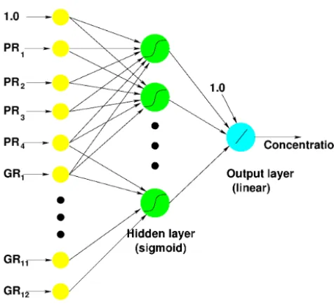
wherefi is the activation function of the unit (also known as a node or a neuron)i. At the hidden layer, the mapping isfi(x)=tanh(x), and at the output layer the mapping is linear, i.e.fo(x)=x. The weights Wij are related to each inputyj. The inputs yj are also outputs from the previous MLP layer (or inputs at the input layer). In the training phase the outputs are first computed in the forward direction, and then the error is propagated back from the MLP output layer, i.e. starting from the error between the ice concentration es-timate given by the MLP and the desired ice concentration defined by the training data, towards the input layer. A de-tailed derivation and presentation of the error backpropaga-tion learning rule can be found, e.g., in Haykin (1999). In our case the only output is the ice concentration, and thus our MLP has only one output unit. In the training phase, the weightsWijare updated towards the negative gradient of the error function at each node. To include a constant term (Wk0), 1.0 is also input into each MLP unit.
J. Karvonen: A sea ice concentration estimation algorithm 1643
Discussion
P
ap
er
|
Discussion
P
ap
er
|
Discussion
P
ap
er
|
Di
scuss
ion
P
ap
er
|
Fig. 2.A schematic diagram of the MLP architecture used, there are 17 input layer units (including the constant term 1.0, 20 hidden layer sigmoid units, and one linear output layer unit. For clarity not all the connection have been drawn in the figure.
28
Figure 2. A schematic diagram of the MLP architecture used; there are 17 input layer units (including the constant term 1.0, 20 hidden-layer sigmoid units and one linear output hidden-layer unit). For clarity not all the connections have been drawn in the figure.
is shown in Fig. 2. The number of the hidden-layer units was determined experimentally: starting from two hidden-layer neurons, then iteratively increasing their number and per-forming the training until the training error did not decrease notably any more by adding more hidden-layer neurons. Be-cause the algorithm makes the estimation segment-wise, not pixel-wise, the estimation is rather fast (in practice it can be run for one mosaic image in a time range of a few seconds to a few tens of seconds on a desktop personal computer, depending on the image and computing power of the com-puter). We used the so-called epoch training (i.e. the whole training data set is iteratively fed through the MLP in a ran-dom order) and each iteration corresponds to one epoch. In the following equations the epochs are indicated by the time variablet, which is an integer number starting from 1. The learning rate parameterµis adaptive. At the first epoch the learning rate is set to 0.005 and it is adjusted after each epoch t depending on the total MLP errorE:
µ(t+1)=1.05µ(t ) if E(t ) < E(t−1), (4) µ(t+1)=0.70µ(t ) if E(t )≥E(t−1). (5) The number of training epochs used was 20 000. The MLP coefficientsWij were initialized randomly, and the MLP co-efficients corresponding to the minimum MLP total errorE among 40 training runs were selected as the final MLP pa-rameters, which are then used in the ice concentration es-timation. This approach guarantees the exclusion of a poor selection of the initial MLP weight coefficient configuration.
4 Evaluation
We evaluated the algorithm results by comparing them to the FMI digitized ice chart grids, which have a nominal resolution of 1 km, and to the high-resolution (3.125 km) UH ASI AMSR-2 algorithm (Beitsch et al., 2013, 2014) re-sults. We also made a visual comparison to the results of the AMSR-2 bootstrap algorithm ice concentrations provided by JAXA (Japan Aerospace eXploration Agency) (Maeda, 2013; JAXA, 2013), which have a resolution of 10 km. The bootstrap algorithm uses the AMSR-2 channels of 36.5 GHz V (vertical), 36.5 GHz H (horizontal), 18.7 GHz V and 23.8 GHz V for the weather filter. We also performed some comparisons over an Arctic Sea test area (Kara and Barents seas), over which we made daily SAR mosaics. We used the same training data as used for the Baltic Sea, and the comparison to the AMSR-2 level 2 concentration results showed good agreement based on visual judgment: the high-and low-concentration areas in general corresponded to each other.
A comparison between SAR-based ice concentration and reference data was made by using three error measures:L1 errorEL1; the signedL1errorEsgn(describing the bias); and root mean square (rms) errorERMS:
EL1 = 1 Ns
Ns X
i=1 C
est i −C
ref i
, (6)
Esgn= 1 Ns
Ns X
i=1
Ciest−Ciref, (7)
ERMS= v u u t
1 Ns
Ns X
i=1
Ciest−Ciref2. (8)
Ns is the number of pixels or grid cells computed over the whole ice concentration estimate grid area,Ciestis the esti-mated concentration andCirefis the reference concentration at each pixel indicated by the indexi. The error measures were computed over the SAR image mosaic area (with a grid cell spacing of 500 m), and the reference data were sampled at the same resolution by using bilinear sampling. The com-parisons were also grid-cell-based comcom-parisons in the SAR mosaic resolution of 500 m.EL1(≥0)describes the mean ab-solute error, andEsgndescribes the bias or systematic error. IfEsgn<0, the algorithm underestimates, and ifEsgn>0, the algorithm overestimates the ice concentration compared to the reference data. The RMSE represents the sample stan-dard deviation of the differences between the estimated val-ues and the reference valval-ues.
1644 J. Karvonen: A sea ice concentration estimation algorithm
Table 1. Errors for our algorithm results compared to FMI ice charts for the training and test data sets. The latitude range of the area is
56–66◦N and the longitude range 16–31◦E; the results were
com-puted for data rectified to Mercator projection with a resolution of 500 m. For both the data sets (training and test sets) the number of
scenesN=10.
Measure Signed error L1error RMSE
Training data set
Error 2.95 8.67 19.98
SD 3.33 2.02 2.42
Test data set
Error −3.91 8.66 21.28
SD 2.67 1.98 3.29
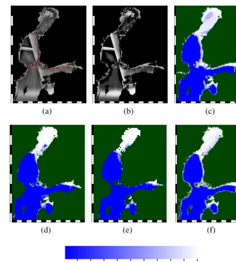
percentage points); the meanL1error for the training and test data sets is practically the same, about 8.7 percentage points. The standard deviations of the errors are relatively low for all the error measures, indicating that the errors are quite simi-lar for all the data. Two examples of the estimation result, the corresponding FMI ice chart concentrations and the cor-responding bootstrap algorithm concentration estimates can be seen in Figs. 3 and 4. In the SAR mosaic and segmenta-tion result (see Fig. 3), we can see that the open-water areas produce different backscattering, depending on the prevail-ing wave conditions, and this can be seen as clear SAR frame boundaries in the open-water areas of the SAR image mosaic and as many separate open-water segments in the segmenta-tion result. However, in the ice-covered areas the SAR frame boundaries are not visible, indicating that the incidence an-gle correction for sea ice has been successful. The ice edge has been sketched as a red line in the SAR mosaic of Fig. 3a; the ice-covered area is in the northern and eastern side of the ice edge line. This indicates that the ice segments can be identified correctly over SAR frame boundaries in the mo-saic, enabling computation of statistics and classification of the ice classes, and they are also separated from open-water segments. In Figs. 3 and 4, we can, for example, see that the new algorithm is unable to capture parts of the ice-covered areas in the northern parts of the Gulf of Finland (latitude around 60◦N). These areas are separated from open water by the SAR segmentation, but, as they are located near the coast, they are problematic for a radiometer at a low resolu-tion (mixed pixels); for this reason the near-coast radiometer pixels are omitted. However, after this, to be able to assign a concentration estimate to each SAR segment, the radiome-ter brightness temperatures are extrapolated as described in Sect. 3.2.
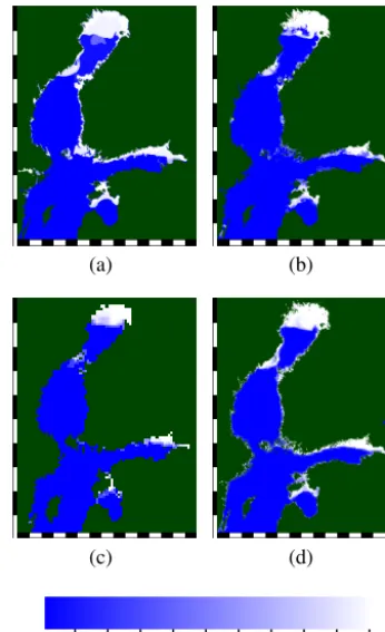
The estimates for the ice zones in the Gulf of Riga (located in the southern part of the images, latitude around 58◦N, longitude 24◦E) correspond to the ice chart concentration much better than the bootstrap algorithm result in both cases
Discussion
P
ap
er
|
Discussion
P
ap
er
|
Discussion
P
ap
er
|
Di
scuss
ion
P
ap
er
|
(a) (b) (c)
(d) (e) (f)
Fig. 3.SAR image mosaic of Feb. 2, 2014, ©MDA (a), the ice edge has been indicated by the red line, segmentation result (b), FMI ice chart grid ice concentration (c),ice concentration estimate using our algorithm (d), AMSR-2 bootstrap algorithm ice concentration give in 10km resolution (e), ASI ice concentration (f). In the image scales the interval is one degree in both latitude and longitude, the upper left corner is (66oN,16oE) and lower right corner (56oN,31oE).
29
Figure 3. SAR image mosaic of 2 February 2014,©MDA (a), the
ice edge has been indicated by the red line; segmentation result (b); FMI ice chart grid ice concentration (c); ice concentration estimate using our algorithm (d); AMSR-2 bootstrap algorithm ice concen-tration given at a 10 km resolution (e); ASI ice concenconcen-tration (f). In
the image scales the interval is 1◦in both latitude and longitude;
the upper left corner is located at 66◦N, 16◦E, and the lower right
corner is located at 56◦N, 31◦E.
J. Karvonen: A sea ice concentration estimation algorithm Discussion 1645
P
ap
er
|
Discussion
P
ap
er
|
Discussion
P
ap
er
|
Di
scuss
ion
P
ap
er
|
(a) (b)
(c) (d)
Fig. 4.FMI ice chart concentration grid for Feb. 11, 2014 (a), ice concentration estimate using our algorithm (b), AMSR-2 bootstrap algorithm ice concentration (c), and ASI ice concentration (d). In the image scales the interval is one degree in both latitude and longitude, the upper left corner is (66oN,16oE)
and lower right corner (56oN,31oE).
30
Figure 4. FMI ice chart concentration grid for 11 February 2014 (a); ice concentration estimate using our algorithm (b); AMSR-2 boot-strap algorithm ice concentration (c); and ASI ice concentration (d).
In the image scales the interval is 1◦in both latitude and longitude;
the upper left corner is located at 66◦N, 16◦E, and the lower right
corner is located at 56◦N, 31◦E.
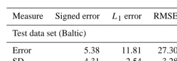
boundaries (ice edge), which have higher precision in FMI ice charts as well as in our combined radiometer–SAR prod-uct. The numerical results of this comparison are given in Tables 2 and 3. We also performed this comparison in the ASI products resolution, and the error measures were 2.64, 10.80 and 22.95 percentage points for the signed error, L1 error and RMSE, respectively.
In some open-water areas in the western parts of the Arc-tic test area mosaic over the Kara and Barents seas, some overestimations of the ice concentration occur, e.g. the open-water area in the mid-left part of the images of Figs. 8b and 9. around an approximate coordinate location (x,y)=(200, 800). These are probably due to different weather conditions and open-water signatures than in the Baltic Sea (training data set) and would probably be corrected by also including data from the Arctic in the training phase. Arctic training data were not used in this study, because we did not have Arctic high-resolution ice chart concentrations available. The Arc-tic test was made just to see whether we can get reasonable results using the Baltic Sea training data. Also, in the Arctic, data sources other than ice charts must be used for training; these could be, for example, ASI or some other radiometer-based concentration results.
Discussion
P
ap
er
|
Discussion
P
ap
er
|
Discussion
P
ap
er
|
Di
scuss
ion
P
ap
er
|
(a) (b)
(c) (d)
Fig. 5.A detail of the Feb. 2, 2014 concentration estimates near the ice edge. FMI ice chart concentration (a), our algorithm result (b), bootstrap ice concentration (c), and ASI ice concentration (d). In the image scales the interval is one degree in both latitude and longitude, the upper left corner is (66oN,16oE) and
lower right corner (56oN,31oE).
31
Figure 5. A detail of the 2 February 2014 concentration estimates near the ice edge. FMI ice chart concentration (a); our algorithm result (b); bootstrap ice concentration (c); and ASI ice
concentra-tion (d). In the image scales the interval is 1◦in both latitude and
longitude; the upper left corner is located at 66◦N, 16◦E, and the
lower right corner is located at 56◦N, 31◦E.
In general it can be said that our algorithm results are slightly better than the ASI results when compared to the FMI ice chart grids. This was an expectable result because we have used FMI ice charts in training of our algorithm. The error measures for the ASI algorithm results compared to FMI ice chart grid results are a bit larger, as shown in Ta-bles 2 and 3.
1646 J. Karvonen: A sea ice concentration estimation algorithm
Table 2. Errors for our algorithm results compared to ASI ice con-centrations for the test data set and for two Arctic Ocean cases (cor-responding to two daily SAR mosaics). The results were computed for data rectified to polar stereographic projection with a resolution of 500 m.
Measure Signed error L1error RMSE
Test data set (Baltic)
Error −1.23 11.15 25.19
SD 7.84 4.15 5.35
Arctic Ocean test cases
Error −3.29 6.68 16.85
SD 5.56 4.20 5.98
Table 3. Errors for the comparison between FMI ice charts and the ASI results. The same Mercator projection as in the other Baltic Sea comparisons was used.
Measure Signed error L1error RMSE
Test data set (Baltic)
Error 5.38 11.81 27.30
SD 4.31 2.54 3.28
The comparisons to the bootstrap ice concentrations pro-vide by JAXA were visual evaluations of the differences. The results of our algorithm correspond to the results of the bootstrap algorithm quite well, based on a general vi-sual overview, but there are still some visible differences, es-pecially in details due to different resolutions of the prod-ucts. However, our algorithm also gives ice estimates for the coastal areas and at the boundaries of different ice con-centration zones in the SAR mosaic resolution. The results of our algorithm and bootstrap ice concentrations are also seen in Figs. 3 and 4. We did not make numerical compar-isons, because of the significantly different resolutions; in this case the effect of the resolution would probably have contributed more to the computed error than the actual er-ror. Some rough estimates of the effect of the different res-olutions to the concentration estimation error can be found, e.g., in Karvonen (2014). To improve the performance, more training data both from the Arctic and the Baltic Sea includ-ing different weather and ice conditions would be required to make a representative data set of the possible weather and ice conditions. Also, studies on using the radiometer data sam-pled at a higher resolution (similar to ASI) will be used to improve the algorithm performance in the future.
We also made a visual comparison for two ice concentra-tion estimaconcentra-tions over an Arctic Ocean test area in the Bar-ents and Kara seas. Also, in these areas, the bootstrap algo-rithm concentrations and concentrations produced by our al-gorithm were in good agreement – as an example, see Fig. 8
Discussion
P
ap
er
|
Discussion
P
ap
er
|
Discussion
P
ap
er
|
Di
scuss
ion
P
ap
er
|
(a) (b)
Fig. 6.Difference between the algorithm result and FMI ice chart concentration for Feb 2, 2014 (a), and between the algorithm result and ASI concentration (b). Overestimation produced by our algorithm with respect to the reference data is indicated by the blue tones (negative difference values) and underestima-tion by red (positive values). In the image scales the interval is one degree in both latitude and longitude,
the upper left corner is (66oN,16oE) and lower right corner (56oN,31oE).
32
Figure 6. Difference between the algorithm result and FMI ice chart concentration for 2 February 2014 (a) and between the algorithm result and ASI concentration (b). Overestimation produced by our algorithm with respect to the reference data is indicated by the blue tones (negative difference values) and underestimation by red
(pos-itive values). In the image scales the interval is 1◦in both latitude
and longitude; the upper left corner is located at 66◦N, 16◦E, and
the lower right corner is located at 56◦N, 31◦E.
Discussion
P
ap
er
|
Discussion
P
ap
er
|
Discussion
P
ap
er
|
Di
scuss
ion
P
ap
er
|
(a) (b)
Fig. 7.Difference between our algorithm result and FMI ice chart concentration for Feb 11, 2014 (a), and between the our result and ASI concentration (b). Overestimation produced by our algorithm with respect to the reference data is indicated by the blue tones (negative difference values) and underestimation by red (positive values). In the image scales the interval is one degree in both latitude and longitude, the
upper left corner is (66oN,16oE) and lower right corner (56oN,31oE).
33
Figure 7. Difference between our algorithm result and FMI ice chart concentration for 11 February 2014 (a) and between our re-sult and ASI concentration (b). Overestimation produced by our al-gorithm with respect to the reference data is indicated by the blue tones (negative difference values) and underestimation by red
(pos-itive values). In the image scales the interval is 1◦in both latitude
and longitude; the upper left corner is located at 66◦N, 16◦E, and
the lower right corner is located at 56◦N, 31◦E.
– even though the training was performed with a rather lim-ited set of Baltic Sea data. We also compared our algorithm results to the ASI high-resolution results over this area for our two test images; the resulting difference map for the case shown in Fig. 8 is shown in Fig. 9. For this comparison we also give the error statistics in Table 2, but due to a very small Arctic data set these values are not very confident.
J. Karvonen: A sea ice concentration estimation algorithm 1647
Discussion
P
ap
er
|
Discussion
P
ap
er
|
Discussion
P
ap
er
|
Di
scuss
ion
P
ap
er
|
(a) (b)
(c) (d)
Fig. 8.An example of the Arctic ocean ice concentration estimation, the SAR mosaic of Feb 2, 2014 (a), ice concentration estimate based on our algorithm (b), the AMSR-2 level 2 ice concentration product (c), and ASI ice concentration product (d). Some parts of the area are not covered by the SAR mosaic (indicated by black tone, such as the land mask, in the mosaick image) and the concentration of our product is only given in the area of the SAR mosaic cover. The image scale interval is 200km, the whole image size is 2200km (x-direction, horizontal) and 1850km (y-direction, vertical). The origin of the coordinate system referred in the text is at the lower left corner.
34
Figure 8. An example of the Arctic Ocean ice concentration esti-mation: the SAR mosaic of 2 February 2014 (a); ice concentration estimate based on our algorithm (b); the AMSR-2 level 2 ice con-centration product (c); and ASI ice concon-centration product (d). Some parts of the area are not covered by the SAR imagery in the SAR mosaic (these areas are indicated by black tone in the SAR mosaic as is the land mask area. Areas not covered by SAR imagery appear in the upper part of the mosaic area and also in the lower right part of the mosaic) and the concentration of our product is only given in the area of the SAR mosaic cover. The image scale interval is
200 km; the sides of the whole image are 2200 km (xdirection,
hor-izontal) and 1850 km (ydirection, vertical) long. The origin of the
coordinate system referred to in the text is at the lower left corner.
locations. The concentration distributions for our algorithm have less mid-range concentration values compared to the bootstrap algorithm and the ASI algorithm, and the differ-ence is larger for the bootstrap algorithm. This is due to the reduced blurring at the (open-water and ice) edges. Because of its high resolution, less edge blurring is generated by our algorithm.
5 Discussion
The results from the comparison to FMI ice charts were bet-ter than, for example, those reported for dual-polarized SAR data in Karvonen (2014). The best concentration estimates can very likely be achieved by combining SAR data and us-ing radiometer data as a background value, such as has been done with the ice thickness values in Karvonen et al. (2008), where modelled sea ice thickness is used as background
Discussion
P
ap
er
|
Discussion
P
ap
er
|
Discussion
P
ap
er
|
Di
scuss
ion
P
ap
er
|
Fig. 9.The difference between the FMI algorithm concentration and ASI ice concentration for the Arctic study area, Feb 2, 2014. The values in the areas where our algorithm indicates higher concentration than ASI appear as blue and areas where our algorithm indicates lower concentration appear as red. The image scale interval is 200km, the whole image size is 2200km (x-direction, horizontal) and 1850km (y-direction, vertical).
35
Figure 9. The difference between the FMI algorithm concentra-tion and ASI ice concentraconcentra-tion for the Arctic study area, 2 Febru-ary 2014. The areas where our algorithm indicates higher concen-tration than ASI appear as blue, and areas where our algorithm in-dicates lower concentration appear as red. The image scale interval
is 200 km; the sides of the whole image are 2200 km (xdirection,
horizontal) and 1850 km (ydirection, vertical) long.
information and SAR imagery is used to improve the reso-lution of the estimates. The methodology may differ, but the basic idea is to enhance the background information based on SAR data to yield more precise estimates in a higher res-olution compared to the background data resres-olution.
1648 J. Karvonen: A sea ice concentration estimation algorithm
methodology for providing high-resolution operational ice concentration estimates.
We have used the resampled AMSR-2 L1R (Level 1 Re-sampled) data which have a resolution of about 10 km. We can see that the ASI algorithm utilizing the full AMSR-2 res-olution (full resres-olution of the higher-frequency channels) is capable of distinguishing details which are not all visible in the L1R data. It would be desirable to use the best possi-ble resolution in the future operational algorithm, and we are going to adapt our MLP algorithm to work with the high-precision data also. After this high-resolution radiometer es-timate we can still refine the segment boundaries based on SAR data to yield improved precision. Actually, all we need to do is to train the algorithm with suitably sampled high-resolution data for a representative training data set; after this it is capable of utilizing the full resolution.
The comparison results show that our algorithm estimates are closer to the FMI ice charts than the other two reference algorithms (bootstrap and ASI). This was an expected result, because the FMI ice charts are mainly based on visual inter-pretation of SAR data, and FMI ice charts and SAR data have been used in the training; thus our algorithm has in a way been adapted to the FMI ice charts.
We were also surprised by the good estimation results in the Arctic test area because the training data were from a rel-atively short period and from the Baltic Sea area. This can at least be partly explained by the fact that, in our Arctic test area, mainly only seasonal sea ice exists; only a little (less than 1 % of the whole image area) multi-year ice can appear in the northeastern parts of the area. In areas with more multi-year ice, the algorithm should be trained with similar data for reliable ice concentration estimates. Because in the Arctic, we do not have digitized ice charts at our disposal, we should use other data sources for the training. One such data source could be the results of other radiometer ice concentration al-gorithms, such as the bootstrap and ASI algorithms used as reference data here, refined by SAR imagery as presented in Sect. 3.3.
The advantage of the MLP approach is that it is not neces-sary to define parameters related to the brightness tempera-tures or ratios; all we need is a representative training data set to train the MLP. The disadvantage is that the actual nonlin-ear mapping from the input parameters to ice concentration remains unknown. The mapping is naturally described by the MLP weights and MLP structure, but the physical relation-ship between inputs and outputs remains unclear.
The novel method results in improved accuracy of the boundaries of the ice zones. As can be seen, the largest differ-ences between our algorithm results and the reference prod-ucts typically appear at the boundaries of the segments corre-sponding to the ice edge. This indicates that our algorithm is capable of representing the boundaries of regions with differ-ent concdiffer-entrations at a resolution defined by the SAR mosaic resolution. There are still some differences when compared to ice chart concentrations, especially in the coastal zones.
This can be explained by the low resolution of the radiome-ter data: in the case of a narrow ice zone near the coast, the ice concentration is highly underestimated by our algorithm. This may be due to the narrow shape of the ice zone along the coastline, which is excluded by the land masking. These con-centrations are better estimated by the 3 km ASI algorithm, indicating that using higher-resolution AMSR-2 data in our algorithm would also probably improve the estimation in the coastal areas. Also, there seem to be some low-concentration areas produced by our algorithm in areas where the ice charts indicate much higher concentrations, for example the area in Fig. 3, approximately around 64◦N, 23◦E. It is very difficult to say whether these segments are due to the more precise distinguishing capability of the algorithm (when the ice an-alyst has given a concentration value for a larger polygon) or to an estimation error (e.g. due to wet snow or water over the ice). In any case, the use of segment-wise brightness tem-perature value modes seems to improve the ice concentration estimation significantly compared to radiometer data alone with respect to the gridded ice chart concentrations. It can be expected that applying our algorithm to radiometer data at a higher resolution would lead to even better results; then the concentration of smaller ice areas and concentration areas near coasts would be estimated better.
6 Conclusions
We have developed an algorithm combining sea ice concen-tration estimates based on radiometer data and SAR segmen-tation to yield high-resolution ice concentration estimates. The radiometer-based estimates are computed in the resolu-tion defined by the radiometer data, and then the estimates are updated using the SAR segmentation. The results are given in the resolution defined by the SAR segmentation. In this experiment we have used an MLP neural network to esti-mate ice concentration from the radiometer data, but, in prin-ciple, any ice concentration estimation could be combined to the SAR segmentation.
The estimation results were compared to the FMI ice charts and ASI algorithm estimates for an independent test data set. The differences when compared to FMI ice chart ice concentrations and to ASI ice concentrations were on av-erage relatively small. The differences were a bit smaller for the FMI ice chart data than for the ASI data. Because the FMI ice charts have been used as a training data set, the al-gorithm has been adapted to the ice concentration estimates given by the FMI ice analysts in the ice charts. The most sig-nificant differences when compared to the reference data sets occur at the boundaries of different ice concentration zones and near the sea–land boundaries.
J. Karvonen: A sea ice concentration estimation algorithm 1649
larger than for the Baltic Sea, but even using only Baltic Sea training data the results were surprisingly good, and we ex-pect better results after training the MLP with Arctic data. (Because we do not have high-resolution ice charts available over the Arctic, we have to use suitably filtered radiometer-based ice concentration data in the training.) The comparison results are presented in detail in Sect. 4.
If fresh SAR data are available, it is useful to refine radiometer-based ice concentration estimates using the SAR data to refine the estimates. This is necessary, for example, for navigation to get concentration estimates on a scale closer to the ship scale.
Due to the promising results we are going to implement this kind of operational ice concentration estimation algo-rithm at FMI in the near future. In our operational algoalgo-rithm we are going to use the AMSR-2 data sampled at the resolu-tion defined by the AMSR-2 89 GHz channel, as in the ASI algorithm, to further improve the estimates. The algorithm will mostly rely on the European Space Agency’s (ESA) Sentinel-1 C-band SAR data and will be run over the Baltic Sea and some Arctic areas for which SAR data are available.
Acknowledgements. Thanks to L. Kaleschke for his constructive
comments and editing the manuscript.
Edited by: L. Kaleschke
References
Beitsch, A., Kaleschke, L., and Kern, S.: AMSR2 ASI 3.125 km Sea Ice Concentration Data, V0.1, Institute of Oceanography, Uni-versity of Hamburg, Germany, digital media, available at: ftp: //ftp-projects.zmaw.de/seaice/ (last access: 31 July 2014), 2013. Beitsch, A., Kaleschke, L., and Kern, S.: The February 2013 Arctic
Sea Ice Fracture in the Beaufort Sea – a case study for two differ-ent AMSR2 sea ice concdiffer-entration algorithms, Remote Sensing, 6, 3841–3856, 2014.
Berg, A.: Spaceborne SAR in Sea Ice Monitoring: Algorithm Devel-opment and Validation for the Baltic Sea, Licentiate thesis, Tech-nical Report 47L, Chalmers University of Technology, Gothen-burg, Sweden, 2011.
Berthod, M., Kato, Z., Yu, S., and Zerubia, J.: Bayesian image clas-sification using Markov Random Fields, Image Vision Comput., 14, 285–295, 1996.
Besag, J.: On the statistical analysis of dirty pictures, J. Roy. Stat. Soc. B, 48, 259–302, 1986.
Bovith, T. and Andersen, S.: Sea Ice Concentration from Single-Polarized SAR data using Second-Order Grey Level Statistics and Learning Vector Quantization, Scientific Report 05-04, Dan-ish Meteorological Institute, Copenhagen, Denmark, 2005. Cavalieri, D. J., Gloersen, P., and Campbell, W. J.: Determination
of sea ice parameters with the NIMBUS 7 SMMR, J. Geophys. Res., 89, 5355–5369, 1984.
Cavalieri, D. J., Markus, T., Hall, D. K., Gasiewski, A. J., Klein, M., and Ivanoff, A.: Assessment of EOS Aqua AMSR-E Arctic Sea
Ice Concentrations Using Landsat-7 and Airborne Microwave Imagery, IEEE T. Geosci. Remote, 44, 3057–3069, 2006. Clausi, D. A.: Comparison and fusion of co-occurrence, Gabor, and
MRF texture features for classification of SAR sea ice imagery, Atmos. Oceans, 39, 183–194, 2001.
Clausi, D. A. and Jernigan, M. E.: Designing Gabor filters for opti-mal texture separability, Pattern Recogn., 33, 1835–1849, 2000. Comiso, J. C.: Characteristics of Arctic winter sea ice from
satel-lite multispectral microwave observations, J. Geophys. Res., 91, 975–994, 1986.
Comiso, J. C.: SSM/I Sea Ice Concentrations Using the Bootstrap Algorithm, NASA Reference Publication/Goddard Space Flight Center 1380, Greenbelt, Maryland, USA, 1995.
Deng, H. and Clausi, D. A.: Gaussian MRF rotation-invariant fea-tures for image classification, IEEE T. Pattern Anal., 26, 951– 955, 2004.
Deng, H. and Clausi, D. A.: Unsupervised segmentation of synthetic aperture radar sea ice imagery using a novel Markov random field model, IEEE T. Geosci. Remote, 43, 528–538, 2005.
Dokken, S. T., Hakansson, B., and Askne, J.: Inter-comparison of Arctic Sea ice concentration using RADARSAT, ERS, SSM/I and in-situ data, Can. J. Remote Sens., 26, 521–536, 2000. Drüe, C. and Heinemann, G.: High-resolution maps of the sea-ice
concentration from MODIS satellite data, Geophys. Res. Lett., 31, L20403, doi:10.1029/2004GL020808, 2004.
Haralick, R. M., Shanmugam, K., and Dinstein, I.: Textural features for image classification, IEEE T. Syst. Man Cyb., SMC-3, 610– 621, 1973.
Haykin, S. S.: Neural Networks, a Comprehensive Foundation, 2nd Edn., Prentice Hall, Upper Saddle River, N.J., USA, 183–196, 1999.
Hornik, K., Stinchcombe, M., and White, H.: Multilayer feedfor-ward networks are universal approximators, Neural Networks, 2, 359–366, 1989.
JAXA: Descriptions of GCOM-W1 AMSR2 Level 1R and Level 2 Algorithms, Rev.A, available at: http://suzaku.eorc.jaxa.jp/ GCOM_W/data/data_w_algorithm.html (last access: 31 July 2014), 2013.
Kaleschke, L. and Kern, S.: ERS-2 SAR Image Analysis for Sea Ice Classification in the Marginal Ice Zone, Proc. IEEE Interna-tional geoscience and remote sensing symposium 2000 (IGARSS 2000), V, 3038–3040, 24–28 July, 2000, Honolulu, Hawaii, USA, 2000.
Kaleschke, L., Lupkes, C., Vihma, T., Haarpaintner, J., Bochert, A., Hartmann, J., and Heygster, G.: SSM/I sea ice remote sensing for mesoscale ocean-atmosphere interaction analysis, Can. J. Re-mote Sens., 27, 526–537, 2001.
Karvonen, J.: Baltic Sea ice concentration estimation based on C-Band HH-Polarized SAR data, IEEE J. Sel. Top. Appl., 5, 1874– 1884, doi:10.1109/JSTARS.2012.2209199, 2012.
Karvonen, J.: Baltic Sea ice concentration estimation based on C-Band Dual-Polarized SAR data, IEEE T. Geosci. Remote, 52, 5558–5566, doi:10.1109/TGRS.2013.2290331, 2014.
Karvonen, J., Cheng, B., and Simila, M.: Ice Thickness Charts Pro-duced by C-Band SAR Imagery and HIGHTSI Thermodynamic Ice Model, Proc. of the Sixth Workshop on Baltic Sea Ice Cli-mate, 71–81, 25–28 August 2008, Lammi, Finland 2008. Karvonen, J., Cheng, B., Vihma, T., Arkett, M., and Carrieres, T.:
1650 J. Karvonen: A sea ice concentration estimation algorithm
on SAR data and a thermodynamic model, The Cryosphere, 6, 1507–1526, doi:10.5194/tc-6-1507-2012, 2012.
Kato, Z., Zerubia, J., and Berthod, M.: Satellite Image Classifica-tion Using a Modified Metropolis Dynamics, in: Proceedings of IEEE International Conference on Acoustics, Speech and Signal Processing (ICASSP 92), 3, 23–26 March 1992, San Francisco, California, USA, 573–576, March, 1992.
Leigh, S., Wang, Z., and Clausi, D. A.: Automated ice-water clas-sification using dual polarization SAR satellite imagery, IEEE T. Geosci. Remote, 52, 5529–5539, 2014.
Maass, N. and Kaleschke, L.: Improving passive microwave sea ice concentration algorithms for coastal areas: applications to the Baltic Sea, Tellus, 62A, 393–410, 2010.
MacQueen, J. B.: Some Methods for classification and Analysis of Multivariate Observations, in: Proceedings of 5th Berkeley Sym-posium on Mathematical Statistics and Probability, 21 June–18 July 1965 and 27 December 1965–7 June 1966, University of California Press., 281–297, 1967.
Maeda, T.: AMSR2 L1R Product, JAXA, available at: http://suzaku. eorc.jaxa.jp/GCOM_W/materials/product/AMSR2_L1R.pdf (last access: 31 July 2014), 2013.
Maillard, P., Clausi, D. A., and Deng, H.: Map-guided sea ice mentation and classification using SAR imagery and a MRF seg-mentation scheme, IEEE T. Geosci. Remote, 43, 2940–2951, 2005.
Makynen, M., Manninen, T., Simila, M., Karvonen, J., and Hal-likainen, M.: Incidence angle dependence of the statistical prop-erties of the C-Band HH-Polarization backscattering signatures of the Baltic Sea Ice, IEEE T. Geosci. Remote, 40, 2593–2605, 2002.
Ochilov, S. and Clausi, D. A.: Operational SAR sea-ice classifica-tion, IEEE T. Geosci. Remote, 50, 4397–4408, 2012.
Pichler, O., Teuner, A. S., and Hosticka, B. J.: A comparison of texture feature extraction using adaptive gabor filtering, pyrami-dal and tree structured wavelet transforms, Pattern Recogn., 29, 733–742, 1996.
Rue, H. and Held, L.: Gaussian Markov Random Fields: Theory and Applications, CRC Press, 2005.
Spreen, G., Kaleschke, L., and Heygster, G.: Sea ice remote sens-ing ussens-ing AMSR-E 89-GHz channels, J. Geophys. Res., 113, C02S03, doi:10.1029/2005JC003384, 2008.
Steffen, K., Key, J., Cavalieri, D. J., Comiso, J., Gloersen, P., St. Germain, K., and Rubinstein, I.: The estimation of geophysical parameters using passive microwave algorithms, Ch. 10, in: Mi-crowave Remote Sensing of Sea Ice, edited by: Carsey, F. D., American Geophysical Society/Wiley, Washington D.C., USA, 201–231, 1992.
Yu, Q. and Clausi, D. A.: SAR sea-ice image analysis based on iter-ative region growing using semantics, IEEE T. Geosci. Remote, 45, 3919–3931, 2007.