www.the-cryosphere.net/8/229/2014/ doi:10.5194/tc-8-229-2014
© Author(s) 2014. CC Attribution 3.0 License.
The Cryosphere
Sea-ice extent and its trend provide limited metrics of model
performance
D. Notz
Max Planck Institute for Meteorology, Hamburg, Germany
Correspondence to: D. Notz ([email protected])
Received: 13 May 2013 – Published in The Cryosphere Discuss.: 27 June 2013 Revised: 6 December 2013 – Accepted: 6 January 2014 – Published: 14 February 2014
Abstract. We examine how the evaluation of modelled
sea-ice coverage against reality is affected by uncertainties in the retrieval of sea-ice coverage from satellite, by the usage of sea-ice extent to overcome these uncertainties, and by in-ternal variability. We find that for Arctic summer sea ice, model biases in sea-ice extent can be qualitatively different from biases in sea-ice area. This is because about half of the CMIP5 models and satellite retrievals based on the Bootstrap and the ASI algorithm show a compact ice cover in summer with large areas of high-concentration sea ice, while the other half of the CMIP5 models and satellite retrievals based on the NASA Team algorithm show a loose ice cover. For the Arctic winter sea-ice cover, differences in grid geometry can cause synthetic biases in sea-ice extent that are larger than the observational uncertainty. Comparing the uncertainty aris-ing directly from the satellite retrievals with those that arise from internal variability, we find that the latter by far domi-nates the uncertainty estimate for trends in sea-ice extent and area: most of the differences between modelled and observed trends can simply be explained by internal variability. For absolute sea-ice area and sea-ice extent, however, internal variability cannot explain the difference between model and observations for about half the CMIP5 models that we anal-yse here. All models that we examined have regional biases, as expressed by the root-mean-square error in concentration, that are larger than the differences between individual satel-lite algorithms.
1 Introduction
The evaluation of climate-model simulations against reality is important both to build confidence in future projections from these models and to understand and improve their pos-sible shortcomings. For a useful evaluation, two quantities must be known: first, the real evolution of the variable that is to be evaluated, and second, the degree to which one can ex-pect agreement between simulation and reality in light of the internal variability of the climate system. In this contribution we examine how the evaluation of modelled sea-ice coverage is affected by the incomplete knowledge of both quantities and by the standard approach that is taken to overcome this incomplete knowledge.
The incomplete knowledge of the actual state of the sea-ice cover arises primarily from the difficulty in accurately determining sea-ice concentration from space, which is the only feasible method to obtain daily global data. Because of wide-spread cloud coverage, most often the passive mi-crowave signature of the ocean surface as retrieved from satellites is used to derive the most likely sea-ice concen-tration in a specific area. This passive microwave signature is, however, strongly affected by meltwater at the ice surface and also by surface temperature, wind speed, humidity and other atmospheric properties. Because of these influencing factors, different retrieval algorithms result in different esti-mates of sea-ice concentration in a particular area (see, for example, Comiso et al., 1997; Kwok, 2002; Meier, 2005; Andersen et al., 2007).
reliable “true” state of sea-ice coverage, most studies that aim at evaluating multiple models against reality have resorted to using a quantity called sea-ice extent that differs only min-imally between the various algorithms. This quantity mea-sures the total area of the ocean surface in which significant amounts of sea ice exist. To calculate sea-ice extent in grid-ded data, one usually adds the area of all grid cells with an ice concentration of more than 15 %. Hence, sea-ice extent in a certain area would be the same for an algorithm that sees a sea-ice concentration of, for example, 40 % and for an algo-rithm that sees a sea-ice concentration of 60 %. While sea-ice extent was initially only used to assess the observed long-term evolution of the sea-ice cover (e.g. Zwally et al., 1983; Parkinson et al., 1987), it has now become common practice to use sea-ice extent also as the primary (and often sole) vari-able to assess the quality of modelled sea-ice coverage (e.g. Stroeve et al., 2007, 2012; Massonnet et al., 2012).
Sea-ice extent is always larger than the more direct inte-grative measure sea-ice area, which is simply the total area of the sea-ice cover and as such a much more direct measure of ice coverage. Important physical quantities such as Arctic-wide average albedo, open-water fraction and thus ocean– atmosphere heat exchange depend therefore much more di-rectly on sea-ice area than on the non-linear measure sea-ice extent. This was already acknowledged by early works on satellite remote sensing (cf. Zwally et al., 1983). The focus on sea-ice extent is, as described, nevertheless understand-able since this parameter can be more reliably observed from ships, airplanes and satellites than sea-ice area. This then al-lows both for a better assessment of the long-term (including pre-satellite) evolution of the ice cover and reduces the un-certainty of the observational data against which model sim-ulations are compared.
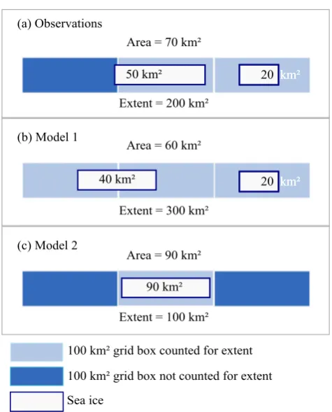
This reduction in uncertainty in the observational data comes, however, at a price, in that sea-ice extent can give misleading results regarding model quality. Consider the triv-ial, fictitious observed sea-ice cover in three grid cells shown in Fig. 1a. Compared to these observations, a model could simulate a smaller sea-ice area that nevertheless results in a larger sea-ice extent because of a slight shift in the location or the spatial distribution of the sea-ice cover (Fig. 1b). A model could also simulate a larger ice area with a smaller sea-ice extent (Fig. 1c). Hence, small shifts in the location of the modelled sea-ice pack, in particular in the marginal ice zone with its strong gradients in sea-ice concentration, can result in misleading results regarding the actual bias in modelled sea-ice cover.
In addition to these grid-independent issues, there is also a grid-dependent issue related to the usage of sea-ice extent vs. sea-ice area. Generally, higher grid resolution causes a lower sea-ice extent. At very high resolution, sea-ice extent converges to the same value as sea-ice area, since then almost all grid cells will either be fully ice covered or fully ice free. We became aware of these issues when we analysed results from the Max Planck Institute for Meteorology Earth System
Area = 70 km²
Extent = 200 km²
Area = 60 km²
Extent = 300 km²
Area = 90 km²
Extent = 100 km²
50 km² 20 km²
40 km²
90 km² (a) Observations
(b) Model 1
(c) Model 2
20 km²
20 km²
20 km²
100 km² grid box not counted for extent
Sea ice
100 km² grid box counted for extent
Fig. 1. A fictitious example to illustrate the possible non-intuitive
relationship between sea-ice area and sea-ice extent. (a) In the ob-servations, the ice pack is distributed such that two grid cells are covered by more than 15 % ice. (b) In a fictitious model simulation, less sea ice than in the observations is distributed such that three grid cells are covered by more than 15 % ice. (c) In a fictitious model simulation, more sea ice than in the observations is distributed such that only one grid cell is covered by more than 15 % ice.
Model MPI-ESM: compared to observations, this model has about 6 % too small a September Arctic sea-ice extent, but 20 % too small a sea-ice area (Notz et al., 2013). In contrast, this model’s predecessor ECHAM5/MPIOM had about 20 % too large a September Arctic sea-ice extent, but only about 7 % too large a sea-ice area. This gave rise to the question of whether too strong a focus on sea-ice extent can give mis-leading results regarding the quality of modelled sea-ice cov-erage, and which implications this has for quantitative model evaluation.
concentration, which avoids such cancellation of errors. We also touch upon the issue of local biases in sea-ice concentra-tion, which are relevant for a more detailed analysis of model quality. Our aim is to allow the reader an informed assess-ment of which parameter to use for a specific purpose and how to handle the related observational uncertainty. In par-ticular, we put our findings into the context of uncertainty that arises because of the internal variability of the Arctic climate system.
The satellite products and the model data that we use are introduced in Sect. 2. In Sect. 3.1, we analyse the compact-ness of the modelled and satellite-retrieved sea-ice cover, which is important to understand the analysis of the different biases in sea-ice extent, area, and in their trends, discussed in Sect. 3.2. In Sect. 3.3, we examine the impact of grid res-olution, followed by an analysis of cancelling negative and positive biases in Sect. 3.4. Section 3.5 then contains an anal-ysis of the impact of internal variability on the assessment of model quality. In Sect. 3.6 we briefly touch upon some issues related to the non-linearity of sea-ice extent. We discuss the implications of these findings for model-evaluation purposes in Sect. 4. Our main findings are then summarised in Sect. 5.
2 Models and data
For our analysis, we focus on the period 1979–2005, which is the overlapping period of the most-widely used satellite records of sea-ice coverage and the “historical” simulations of the CMIP5 protocol (Taylor et al., 2012). These historical simulations are forced by the observed evolution of green-house gases, solar radiation, etc. For all 117 historical simu-lations from 26 different models that we consider here, time series of monthly mean sea-ice extent and area are calcu-lated from their monthly mean sea-ice concentration fields. The sea-ice extent is calculated as the total area of all grid cells with at least 15 % sea-ice concentration. For sea-ice area, the area of all grid cells is multiplied by their sea-ice concentration and then added. For sea-sea-ice area and ex-tent, linear trends are calculated as a least-squares fit to the time series. Ensemble-mean and multi-model mean time se-ries of sea-ice extent and sea-ice area are calculated as the ensemble-mean and the multi-model mean of the individ-ual simulations’ time-series of these two parameters, and not from the ensemble-mean or multi-model mean concentration fields (compare Sect. 3.6).
The model results are compared against satellite retrievals of sea-ice concentration. As described in the introduction, different algorithms result in different estimates of sea-ice concentration because they are based on different transfer functions to derive sea-ice concentration from the measured passive-microwave signature. These differences are best doc-umented (e.g. Comiso et al., 1997; Kwok, 2002) for the two satellite algorithms for sea-ice concentration that are most widely used for model-data intercomparison studies:
the Bootstrap algorithm (Comiso, 1986) and the NASA Team algorithm (Cavalieri et al., 1984) that forms the basis for the NSIDC Sea-Ice Index (Fetterer et al., 2002, updated 2012). Both provide sea-ice concentration data from 1979 onwards, and will be used throughout this study to exemplify the short-comings of a direct comparison of modelled sea-ice extent to one particular satellite algorithm. Additionally, we con-sider retrievals based on the ASI algorithm (Kaleschke et al., 2001; Spreen et al., 2008), which provides sea-ice concentra-tion based on SSM/I data from 1991 onwards and based on AMSR-E data from 2002 onwards.
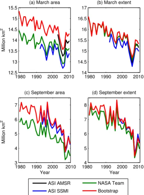
Sea-ice concentration retrieved through the Bootstrap al-gorithm is, especially in summertime, probably closer to the real sea-ice concentration than that from the NASA Team algorithm, because the latter has been found to be biased low compared to independent observations (e.g., Agnew and Howell, 2003; Partington et al., 2003). The Bootstrap algo-rithm, in contrast, results in estimates of sea-ice concentra-tion that are very close to the “Climate Data Record of Pas-sive Microwave Sea Ice Concentration” (CDR, Meier et al., 2011) that is a merged product of different algorithms with the aim to provide a consistent time series of sea-ice con-centration. In summer, estimates of sea-ice area of the Boot-strap algorithm also agree favourably with estimates based on the ASI algorithm from SSMI satellite data and the higher resolved AMSR-E satellite data, while estimates of sea-ice area based on the NASA Team algorithm are significantly lower (Fig. 2). Since all passive-microwave algorithms will see surface melt ponds as open water, their estimates of sea-ice concentration in summer have been found to be lower than independent observations. Comiso and Nishio (2008) have therefore suggested to synthetically increase sea-ice ex-tent by a 25 km-wide margin during the melt season. In line with existing model–satellite intercomparison studies we will not take such a measure for our model-satellite intercompar-ison in Sect. 3. We will, however, return to the issue of the low-bias in satellite retrievals in Sect. 4. There we will also discuss in more detail the greater uncertainty of the retrieved sea-ice area and the differences between the various algo-rithms shown in Fig. 2.
3 Results
3.1 The frequency distribution of sea-ice concentration
1980 1990 2000 2010 12.5
13 13.5 14 14.5 15
15.5 (a) March area
Million
km
2
1980 1990 2000 2010 14
14.5 15 15.5 16 16.5
17 (b) March extent
1980 1990 2000 3
4 5 6 7
(c) September area
Year 1990 2000 2010
4 5 6 7 8
(d) September extent
Year 2010 1980
ASI AMSR ASI SSMI
NASA Team Bootstrap
Million
km
2
Fig. 2. September and March sea-ice area and sea-ice extent as
re-trieved from satellite for the period 1979–2010. Different colors denote different algorithms or satellites. Area and extent were cal-culated based on sea-ice concentration fields on EASE grids with 25 km resolution (NASA Team and Bootstrap, based on SMMR and SMM/I, 1979–2010), 12 km resolution (ASI SSM/I, 1992–2010) and 6 km resolution (ASI AMSR-E, 2002–2010).
with 6.3 million km2for the Bootstrap algorithm compared to only 5.2 million km2for the NASA Team algorithm. This much larger difference is the main reason why the sea-ice area estimate of an individual satellite retrieval is usually not used for model-evaluation purposes. Such large relative dif-ference arises, however, only in summer: in March, both the estimates of sea-ice area and of sea-ice extent are similar be-tween the two algorithms, as the mean 1979–2005 sea-ice extent is 15.9 million km2for Bootstrap and 15.8 million km2 for NASA Team, while sea-ice area is 14.6 million km2 for Bootstrap and 13.9 million km2for NASA Team.
Since our focus here is on sea-ice extent vs. sea-ice area, it is important to understand the cause for the different agree-ment between these two measures for the satellite algorithms. For this purpose, we consider the frequency distribution of sea-ice concentration that is displayed by the two algorithms. Of particular importance for the estimate of sea-ice area is the amount of ice-covered grid cells that have a very high ice concentration. According to the Bootstrap algorithm the
20 40 60 80 100 0
0.2 0.4 0.6 0.8
(a) Bootstrap (September)
20 40 60 80 100 0
0.2 0.4 0.6 0.8
(b) NASA Team (September)
20 40 60 80 100 0
0.2 0.4 0.6 0.8
(c) Bootstrap (March)
20 40 60 80 100 0
0.2 0.4 0.6 0.8
(d) NASA Team (March)
Normalised frequency distribution of sea−ice concentration Sea−ice concentration range [%]
Fig. 3. Histogram of 1979–2005 sea-ice concentration in all
ar-eas with at lar-east 0.1 % sea-ice concentration. (a, c) Satellite trievals based on the Bootstrap algorithm and (b, d) satellite re-trievals based on the NASA Team algorithm for (a, b) September and (c, d) March. The numbers on thexaxis denote the upper limit of each bar: e.g. 20 denotes the concentration range 10 to 20 %.
ice cover is very compact in summer, with about 70 % of all ice-covered grid cells having more than 90 % ice concentra-tion (Fig. 3a). In contrast, according to the NASA Team algo-rithm the ice cover is quite loose, with only about 20 % of all ice-covered grid cells having such high ice concentration in summer (Fig. 3b). This difference comes primarily about by the different treatment of sea ice that is covered by surface meltwater (Meier and Notz, 2010; L. T. Pedersen, personal communication, 2013): while both algorithms interpret the meltwater-covered sea ice as open water, the Bootstrap al-gorithm more strongly compensates for this well-known bias compared to the NASA Team algorithm. The two versions of the ASI algorithm that were analysed for the present study show a similarly compact ice cover as the Bootstrap algo-rithm.
0 0.2 0.4 0.6 0.8
1 ACCESS bcc−csm1 CanCM4 CanESM2 CCSM4 CNRM−CM5 CSIRO−Mk3−6−0
0 0.2 0.4 0.6 0.8
1EC−EARTH GFDL−CM3 GFDL−ESM2G GFDL−ESM2M HadCM3 HadGEM2−CC HadGEM2−ES
0 0.2 0.4 0.6 0.8 1
IPSL−CM5A−LR IPSL−CM5A−MR IPSL−CM5B−LR MIROC4h MIROC5 MIROC−ESM MPI−ESM−LR
20 60 100 0
0.2 0.4 0.6 0.8
1MPI−ESM−MR
20 60 100 MPI−ESM−P
20 60 100 MRI−CGCM3
20 60 100 NorESM1−ME
20 60 100 NorESM1−M
20 60 100 Bootstrap
20 60 100 NASA Team
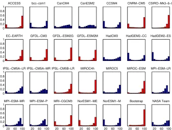
Fig. 4. Histogram of 1979–2005 September sea-ice concentration in all grid cells with at least 0.1 % sea-ice concentration in CMIP5 model
simulations. The numbers on thexaxis denote the upper limit of each bar: e.g. 20 denotes the concentration range 10 to 20 %. Red panels denote histograms with a compact sea-ice cover, while blue panels denote histograms with a loose sea-ice cover. For models with multiple simulations, the ensemble mean is shown.
small both in summer and winter, both algorithms result in similar estimates of sea-ice extent.
Examining the frequency distribution of summer sea-ice concentration in the CMIP5 model simulations, we find that these simulations can be divided into two groups. One group simulates a compact ice cover in summer (red panels in Fig. 4), while the other group simulates a loose ice cover (blue panels in Fig. 4). In winter, all models simulate a com-pact ice cover (not shown). Somewhat arbitrarily, we chose a normalised frequency of 0.4 for the 90. . . 100 % concen-tration band as the dividing line between simulations with a compact ice cover and simulations with a loose ice cover. An alternative definition could be based on the ratio of the amount of sea ice in the highest concentration and that in the second-highest class. Depending on the demarcation line for this ratio, this would slightly modify the composition of the two classes without qualitatively affecting the results dis-cussed in the following.
It would be interesting to examine why roughly half of the CMIP5 models produce a compact ice cover while the other half does not, in particular since this might allow further in-sights into the quality of the satellite retrievals. Some initial analyses point towards the relative distribution of melting be-tween lateral melt and thinning in individual models to play some role, but a conclusive analysis of this question is be-yond the scope of this paper.
What is important, however, is to reiterate the fact that the occurrence of a compact vs. a loose ice cover has dif-ferent implications in the models compared to the satellite retrievals: in the models, this terminology does indeed refer to the actual simulated state of the ice cover. In the satellite retrievals, however, this differentiation is above all a reflec-tion of the different treatment of surface meltwater by the dif-ferent algorithms. An algorithm that interprets more of that meltwater as ice free will necessarily result in an “observed” loose ice cover, though this then has little to say about the real properties of the ice pack.
3.2 Extent vs. area
By nature of the definition of sea-ice extent, differences be-tween sea-ice extent and sea-ice area are comparably small for compact sea ice, because of the large number of grid cells with a very high ice concentration. In contrast, the difference between extent and area is usually much larger for a loose ice cover (see Fig. 5a–c).
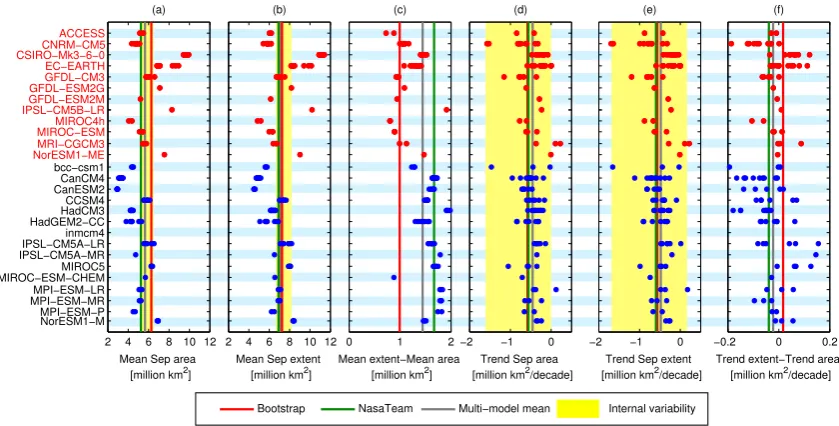
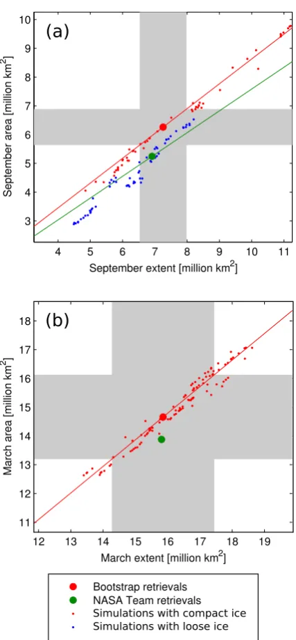
This has direct consequences for the analysis of model bi-ases based on these two measures. We find for simulations with a compact sea-ice cover that biases relative to the Boot-strap retrieval are similar for sea-ice area and sea-ice ex-tent (red dots are close to red line in Fig. 6a). In particular, all simulations with a compact sea-ice cover that are within
2 4 6 8 10 12 ACCESS
bcc−csm1 CanCM4 CanESM2 CCSM4 CNRM−CM5 CSIRO−Mk3−6−0 EC−EARTH GFDL−CM3 GFDL−ESM2G GFDL−ESM2M
HadCM3 HadGEM2−CC inmcm4 IPSL−CM5A−LR IPSL−CM5A−MR IPSL−CM5B−LR MIROC4h
MIROC5 MIROC−ESM−CHEM MIROC−ESM
MPI−ESM−LR MPI−ESM−MR MPI−ESM−P MRI−CGCM3 NorESM1−ME
NorESM1−M
Mean Sep area [million km2]
(a)
2 4 6 8 10 12 Mean Sep extent
[million km2] (b)
0 1 2
Mean extent−Mean area [million km2]
(c)
−2 −1 0
Trend Sep area [million km2/decade]
(d)
−2 −1 0
Trend Sep extent [million km2/decade]
(e)
−0.2 0 0.2 Trend extent−Trend area [million km2/decade]
(f)
Bootstrap NasaTeam Multi−model mean Internal variability
Fig. 5. Overview of the September sea-ice coverage in the 117 historical CMIP5 simulations analysed for this study. Each individual dot
corresponds to a single simulation. The vertical lines show the values of the observational record and the mean of all simulations. The yellow shading indicates estimated internal variability. All data refer to the period 1979–2005. (a) Mean September sea-ice area, (b) mean September sea-ice extent, (c) difference between mean September sea-ice extent and mean September sea-ice area, (d) linear trend in September sea-ice area, (e) linear trend in September sea-ice extent, (f) difference between trend in September sea-ice extent and trend in September sea-ice area. Models with a compact ice cover are labelled in red.
of the retrieved sea-ice area. For the simulations with a loose ice cover, we find that those models that underestimate sea-ice extent relative to the Bootstrap retrieval have a stronger percentage bias in sea-ice area than they have in sea-ice ex-tent, while those simulations that overestimate sea-ice extent have a smaller percentage bias in sea-ice area than in extent (Fig. 6a). A number of simulations with a loose ice cover that fall within±10 % of the retrieved sea-ice extent are clearly outside the±10 % range of the retrieved sea-ice area, and vice versa. Hence, a focus on sea-ice extent can give mis-leading results regarding model quality compared to a focus on sea-ice area (see also Fig. 5a, b, where a number of simu-lations with loose ice match the Bootstrap sea-ice extent well but are below Bootstrap sea-ice area).
Relative to the satellite-retrieved estimates based on the NASA Team algorithm, we find that biases for sea-ice ex-tent are similar to biases for sea-ice area for simulations with a loose ice cover (blue dots close to green line in Fig. 6a). Simulations with a compact ice cover that overestimate the mean sea-ice extent compared to the NASA Team algorithm in contrast have a stronger percentage bias in sea-ice area, and vice versa.
For March, all simulations and both satellite retrievals have a compact ice cover. Hence, percentage biases in sea-ice area are for all simulations almost identical to the biases in sea-ice extent (Fig. 6b).
To understand this behaviour of simulations with a com-pact ice cover vs. those with a loose ice cover, we need to
consider that the former have a small difference between sea-ice extent and sea-sea-ice area, while the latter have a larger dif-ference. Figure 7 illustrates how this explains the different behaviour of the two model families: if any of the loose-ice simulations with their comparably large difference between sea-ice extent and sea-ice area results in too small a mean sea-ice extent, this simulations’ bias in sea-ice area will be comparably large. If, however, the simulation resulted in too large a sea-ice extent, its bias in sea-ice area would be com-parably smaller – simply because the difference between ex-tent and area is larger in the simulations than in the obser-vations. For simulations with a compact ice cover, biases in extent and area relative to the Bootstrap algorithm are very similar, because these simulations’ difference between sea-ice extent and sea-sea-ice area is similar to that of the Boot-strap observations. Compared to observations based on the NASA Team algorithm, the simulations with a compact ice cover have generally a lower difference between extent and area, which explains their contrasting behaviour relative to the NASA Team algorithm.
In winter, all simulations result in a compact sea-ice cover. Therefore, in winter they have a difference between sea-ice extent and sea-ice area similar to the Bootstrap observations, which explains the consistent wintertime biases of all model simulations.
4 5 6 7 8 9 10 11 3
4 5 6 7 8 9 10
September extent [million km2]
September
area
[million
km
2 ]
12 13 14 15 16 17 18 19
11 12 13 14 15 16 17 18
March extent [million km2]
March
area
[millio
n
km
2 ]
Bootstrap retrievals NASA Team retrievals Simulations with compact ice Simulations with loose ice
(b)
(a)
Fig. 6. (a) September and (b) March sea-ice area vs. sea-ice extent
in models and satellite retrievals. The red line connects all value pairs that have the same percentage bias in sea-ice extent and in sea-ice area relative to the Bootstrap retrievals. The gray shading indicates a±10 % range around the values obtained from the Boot-strap retrievals. Note that in March all simulations have compact ice, which is why there are no blue dots in (b).
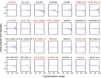
0.56 million km2 per decade in sea-ice extent and a loss of 0.58 million km2per decade in sea-ice area during the period 1979–2005. The models, in contrast, show inconsistent be-haviour, with both smaller and larger trends in sea-ice area than in extent (Fig. 5d, f). The consistent trends in the satel-lite retrieval can be understood by analysing the individual trends for different ice-concentration ranges (Fig. 8). Almost
mi
llion km
²
Compact
Observations Simulation 1
extent
area
Simulation 2
Fig. 7. Schematic to explain the findings in Fig. 6: because of the
smaller difference between sea-ice extent and sea-ice area in obser-vations with a compact ice cover than in simulations with a loose ice cover, models with a loose ice cover and slightly too large a simu-lated sea-ice extent result in a comparably small bias in simusimu-lated sea-ice area. The difference between simulated extent and simulated area is the same for both simulations.
all the ice loss in the Bootstrap retrievals happens within the ice-concentration range 90 to 100 %, with no compen-sating increase in lower ice-concentration ranges (second to last panel in Fig. 8). An ice loss at these high concentrations will have roughly the same impact on ice area and on sea-ice extent. For most models, in contrast, the sea-ice loss is spread over a wider range of sea-ice concentrations. In addition, the grid cells with high ice concentration often only lose some of their ice, which then causes an increase in the number of grid cells with intermediate ice concentration. This compen-sation then causes a smaller loss of sea-ice extent than of sea-ice area. Some models, however, also show a faster loss in sea-ice extent than in sea-ice area. This behaviour can be understood if a significant amount of grid cells with interme-diate sea-ice concentration become ice free in a simulation. The entire area of these grid cells is then lost in terms of sea-ice extent, while only the fraction of these grid cells that was ice-covered is lost from sea-ice area.
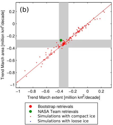
The different biases in trends of area and extent in mod-els vs. the satellite retrievals obviously have consequences for the assessment of model quality (Fig. 9a). A number of simulations result in trends that lie within±20 % of the Boot-strap retrieved trends in sea-ice extent, while they lie outside the±20 % range for the simulated trends in sea-ice area. In particular, models that have too fast a loss in sea-ice extent compared to Bootstrap retrievals sometimes have too slow a loss in sea-ice area compared to the Bootstrap retrievals. The same holds for the trends in winter sea-ice coverage (Fig. 9b). Hence, again, an assessment of model quality based on an analysis of trends in sea-ice extent can give misleading re-sults.
3.3 Grid resolution
−1 −0.5 0 0.5
1 ACCESS bcc−csm1 CanCM4 CanESM2 CCSM4 CNRM−CM5 CSIRO−Mk3−6−0
−1 −0.5 0 0.5
1EC−EARTH GFDL−CM3 GFDL−ESM2G GFDL−ESM2M HadCM3 HadGEM2−CC HadGEM2−ES
−1 −0.5 0 0.5 1
IPSL−CM5A−LR IPSL−CM5A−MRIPSL−CM5B−LR MIROC4h MIROC5 MIROC−ESM MPI−ESM−LR
20 60 100
−1 −0.5 0 0.5
1MPI−ESM−MR
20 60 100
MPI−ESM−P
20 60 100
MRI−CGCM3
20 60 100
NorESM1−ME
20 60 100
NorESM1−M
20 60 100
Bootstrap
20 60 100
NASA Team
concentration range
Tr
en
d
[m
illi
on
k
m
2/d
eca
de
]
Fig. 8. Trends in September sea-ice area per ice-concentration category. The numbers on thexaxis denote the upper limit of each bar: e.g. 20 denotes the concentration range 10 to 20.
between sea-ice extent and sea-ice area for higher grid res-olution. The comparably high resolution of the satellite data set might therefore have contributed to the comparably small difference between sea-ice area and sea-ice extent for the Bootstrap algorithm (Fig. 5c).
To examine this possibility, we bilinearly interpolated the gridded Bootstrap-derived sea-ice concentration field for each month of the year 2007 from the original 25 km EASE grid to each individual model grid and then calculated area and extent on the model grids. We find that sea-ice area usu-ally agrees well between the original grid and the individ-ual model grids, with a multi-model mean difference of less than 50 000 km2 all year round (blue line in Fig. 10). Indi-vidual models typically show a mean difference of less than 200 000 km2all year round, where the difference compared to the original EASE grid comes primarily about through roundoff errors, which is also exemplified by the fact that both positive and negative differences occur. Sea-ice extent as calculated from the interpolated sea-ice concentration on the lower-resolved model grids, however, is always larger than the one on the original 25 km EASE grid. In particular in winter, the multi-model mean difference reaches more than 800 000 km2, decreasing to less than 200 000 km2around the summer minimum (red line in Fig. 10). For the calculation of sea-ice extent, grid resolution and grid geometry can hence strongly affect the comparison between model simulations and satellite retrievals for the large ice cover that is still typi-cal for wintertime.
3.4 Cancelling biases
So far, we have examined possible misinterpretations that can arise when using sea-ice extent instead of sea-ice area for model-evaluation purposes. However, both measures al-low for cancelling biases and hence render a regional assess-ment of model quality difficult: a model that has a large pos-itive bias in sea-ice concentration in one region and a large negative bias in another region might simulate a better over-all sea-ice area than a model that has weak negative biases in both regions. Therefore, an analysis of the mean absolute bias in sea-ice concentration gives a better indication of re-gional model performance compared to either sea-ice extent or sea-ice area.
−1.2 −1 −0.8 −0.6 −0.4 −0.2 0 −1.2
−1 −0.8 −0.6 −0.4 −0.2 0
Trend September extent [million km2/decade]
Trend
Septemb
er
area
[million
km
2 /decade]
−1 −0.8 −0.6 −0.4 −0.2 0 0.2
−1 −0.8 −0.6 −0.4 −0.2 0 0.2
Trend March extent [million km2/decade]
Trend
March
are
a
[million
km
2 /decade]
Bootstrap retrievals NASA Team retrievals
Simulations with compact ice Simulations with loose ice
(b)
(a)
Fig. 9. (a) September and (b) March trends in sea-ice area vs. trends
in sea-ice extent for the period 1979–2005. The red line connects all value pairs that have the same percentage bias in sea-ice extent and in sea-ice area relative to the Bootstrap retrievals. The gray shad-ing indicates a±20 % range around the trends obtained from the Bootstrap retrievals.
for the linear regression of area vs. mean concentration is pri-marily related to interpolation issues during the calculation of mean biases.
For the absolute biases in sea-ice concentration that pre-vent the cancellation of regional biases, however, correlation with the absolute percentage bias in the integrative measures sea-ice extent and sea-ice area is low, givingR2≈0.5 for both measures: some models with almost no bias in sea-ice
0 2 4 6 8 10 12
0 0.1 0.2 0.3 0.4 0.5 0.6 0.7 0.8 0.9
Month
Interpolated − original grid [million km
2 ] Extent .
Area
Fig. 10. Mean difference of sea-ice area and sea-ice extent between
the original 25 km EASE-Grid and all CMIP5 model grids through-out the year 2007. For each month, the Bootstrap-derived sea-ice concentration was interpolated onto all individual model grids, from which then sea-ice extent and sea-ice area were calculated. The dif-ferences of all grids relative to the original EASE-Grid were aver-aged for this figure.
extent or area still have comparably large mean absolute con-centration biases.
For model-evaluation purposes this suggests that addi-tional insights can be gained by considering not only sea-ice area, but also the root mean square bias of the sea-ice concen-tration fields. This allows for some estimate of the quality of modelled regional sea-ice distributions, while the integrated measure sea-ice area allows for an estimate of the quality of the overall sea-ice volume that is formed through the conver-gence and diverconver-gence of heat fluxes across the entire Arctic. Both measures would be particularly insightful if the magni-tude and timing of their seasonal distribution were assessed.
3.5 Internal variability
−60−40−20 0 20 40 60 ACCESS
bcc−csm1 CanCM4 CanESM2 CCSM4 CNRM−CM5 CSIRO−Mk3−6−0 EC−EARTH GFDL−CM3 GFDL−ESM2G GFDL−ESM2M HadCM3 HadGEM2−CC HadGEM2−ES IPSL−CM5A−LR IPSL−CM5A−MR IPSL−CM5B−LR MIROC4h MIROC5 MIROC−ESM MPI−ESM−LR MPI−ESM−MR MPI−ESM−P MRI−CGCM3 NorESM1−ME NorESM1−M
Percentage bias in Sep. area
(a)
−60−40−20 0 20 40 60 Percentage bias
in Sep. extent (b)
−30−20−10 0 10 20 30 Mean bias in Sep. conc.
0 10 20 30
Mean absolute bias in Sep. conc.
(d) (c)
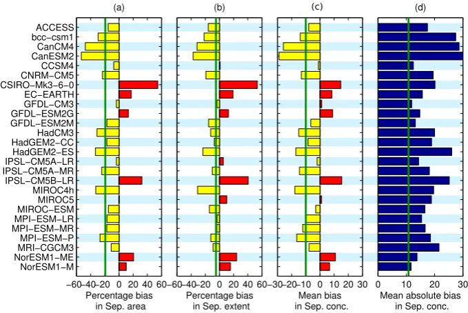
Fig. 11. Overview of biases in September sea-ice coverage in the 117 “historical” CMIP5 simulations analysed for this study relative to
Bootstrap satellite retrievals. (a) Mean bias in September sea-ice area. (b) Mean bias in September sea-ice extent. (c) Mean bias in sea-ice concentration. (d) Mean absolute bias in sea-ice concentration. The vertical green lines denote the respective bias of the NASA Team retrieval relative to the Bootstrap retrieval.
solar activity, aerosol load etc. The only difference between the simulations were the initial weather conditions on the simulated 1 January 1850, which was the starting date for the simulations. This exemplifies the well-known fact that because of the chaotic nature of the climate system, the trend in the response of the climate system to a given trend in the external forcing can vary drastically on short timescales.
Because of this large internal variability of the Arctic cli-mate system it is often impossible to judge whether a dif-ference in sea-ice coverage between a model simulation and observations is simply random or caused by a model defi-ciency (cf. Winton, 2011). While there are observational es-timates of decadal-scale internal variability of the Arctic sea-ice cover (cf. Notz and Marotzke, 2012), a reasonable range of sea-ice trends for previous decades can obviously not ro-bustly be inferred from observations, since only one single trend has been realised by the real world. It is, however, possible to estimate from ensemble model simulations how much of a modelled trend is caused by the external forcing and how much of it is caused by internal variability, and to then translate these results to the real world (e.g. Kay et al., 2011; Day et al., 2012).
Here, we use a simple, straight-forward method to estimate a reasonable range of observed sea-ice area and sea-ice extent and of their trends from our CMIP5 simulation ensemble: we assume that this reasonable range is given by the maximum spread of ensemble simulations of all those models that en-compass the observed evolution within their ensemble mem-bers. While this would ideally be done on a model-by-model
basis, many models that we examine here do only provide a single ensemble member. We therefore generalise the spread from models that do provide multiple ensemble members to all simulations that we consider here.
Using this approach to examine mean September sea-ice area for the period 1979–2005 (yellow shading in Fig. 5a), we find an up to 1 million km2 ensemble spread for those models that match the Bootstrap-observed value of 6.3 million km2 in at least one of their ensemble mem-bers. This spread is comparable to the difference between the Bootstrap- and the NASA-Team-derived sea-ice area. Hence, for the period considered here the reasonable range of mean September sea-ice area as derived from model simulations is similar to the uncertainty range of the satellite observations. Simulations that fall outside of this range are most likely in-compatible with the observed external forcing. Based on this reasoning, 14 of the 26 models that we analysed have too small a sea-ice area for that period in all their ensemble mem-bers, while 5 have too large a sea-ice area in all their ensem-ble members. The mean of all simulations, 5.6 million km2, lies within the reasonable range.
ensemble members, while 4 have too large a sea-ice extent in all their ensemble members. The mean of all simulations, 7.1 million km2, lies again within the reasonable range.
The large number of model simulations that fall outside the reasonable range for both sea-ice extent and sea-ice area indicates that the mean value of these two measures is in prin-ciple helpful for model-evaluation purposes, notwithstand-ing the differences that can arise for individual models for the two measures as discussed above. In contrast, the inter-nal variability of the trends is so large that trends of indi-vidual simulations can hardly be used for model-evaluation purposes (Fig. 5d, e): for the period 1979–2005, many mod-els which generated one simulation with a sea-ice trend sim-ilar to the observed one simulate for identical forcing and slightly different initial conditions trends that are twice as strongly negative, or trends that are even positive. Hence, any trend that falls within this range might be the consequence of internal variability affecting the modelled trend rather than a model deficiency. Using such criterion, almost all simu-lations that we consider here show a trend for the period 1979–2005 that is consistent with the observed increase in greenhouse-gas emissions. Since 2005, Arctic sea-ice cover-age in summer has decreased rapidly. The trend in September sea-ice coverage for the extended period 1979–2012, how-ever, remains below 1 million km2 ice loss per decade both for extent and area. As such, the trend remains comfortably within our estimated range of modelled trends modified by internal variability. Hence, also for the extended temporal range until 2012 we cannot positively identify the modelled trends as inconsistent with the applied forcing.
In their evaluation of CMIP5 simulations, Stroeve et al. (2012) estimate a range for the trend in sea-ice extent that is consistent with the observed external forcing by calculating the standard deviation of the observations around the linear trend. Since the observed trend might be extraordinary for the observed forcing, we here instead assume that the rea-sonable range for the trend is given by the much larger en-semble spread of those models that encompass the observed trend within their ensemble spread. We then take this model ensemble spread to represent the range of possible trends that are consistent with an externally forced trend modified by in-ternal variability over the previous decades. Since we find that almost all simulations that we consider here fall within this wider range of reasonable trends, we conclude that an assessment based on the difference between the observed trend and individual ensemble simulations only allows for very limited insights into model quality.
3.6 Non-linearity
For completing our discussion of the usage of sea-ice ex-tent for model evaluation, we should finally note that for any comparison of modelled mean sea-ice extent with observa-tions, the non-linearity of sea-ice extent must carefully be taken into account. Mean sea-ice extent should normally be
calculated as the mean of the sea-ice extents of the individual simulations, and not as the sea-ice extent of the mean concen-tration of the simulations. Consider, for example, two simula-tions, one with 0 % ice concentration in a certain region and the other with 35 % ice concentration in that same region. The mean ice concentration of these simulations is larger than 15 %, and the sea-ice extent of the mean of the two simu-lations will be identical to the sea-ice extent of the simulation with the higher sea-ice concentration. The same issue arises when directly comparing sea-ice extent from daily observa-tions with monthly mean fields of model output: the monthly-mean sea-ice extent as derived from a monthly-monthly-mean sea-ice concentration field will usually be larger than the monthly mean of daily estimates of sea-ice extent. Therefore for the purpose of this paper, all daily satellite data sets were aver-aged to monthly data before calculating sea-ice extent. Since sea-ice area scales linearly with ice coverage, these issues do not apply for any study using sea-ice area as a metric for model quality.
4 Discussion
In the previous section, we have shown that for a number of reasons the sole consideration of sea-ice extent for the evalu-ation of model quality can give misleading results. We there-fore recommend that future studies that aim at evaluating the performance of sea ice move away from the sole consider-ation of sea-ice extent and also consider the model perfor-mance for the more meaningful integrative quantity sea-ice area.
In doing so, differences between different satellite algo-rithms will play a more prominent role than for sea-ice ex-tent (see Fig. 2). Hence, such comparison will need to take more the form of a comparison of observational data with a specific uncertainty vs. model simulations with a specific in-ternal variability. To quantify the uncertainty of the satellite data, we compared in more detail the four satellite algorithms shown in Fig. 2. We find that despite their large difference in retrieved sea-ice area, these algorithms have a similar year-to-year variability, which becomes apparent if anomalies of all satellite algorithms relative to the retrieved area in 2010 are plotted together (see Fig. 12a, b). Hence, the difference between the satellite products is largely caused by a constant offset and there is larger certainty in anomalies in sea-ice area than there is in its absolute value. This is important for any model simulation with assimilated sea-ice concentration fields: one should expect such a model to at least retrieve the anomaly structure of the satellite time series, which can be very reliably estimated.
1980 1990 2000 2010 −1 0 1 2 3
1980 1990 2000 2010
−1 0 1 2 3 ASI AMSR
ASI SSMI NASA TeamBootstrap
2 4 6 8 10 12
5 10 15
2 4 6 8 10 12
0.6 0.8 1 1.2 1.4
2 4 6 8 10 12
0 0.1 0.2 0.3 0.4 0.5
2 4 6 8 10 12
−2 −1 0 1 year year month month
Anomaly in sea ice area relative to 2010
(a) March (b) September
Mean seasonal cycle 2003-2010
(c) sea-ice area (d) trend in sea-ice area
[m illi on k m 2] [m illi on k m 2] [m illi on k m 2] [m illi on k m 2/d eca de ]
Mean uncertainty 2003-2010
max-min
max-min
2 . std. dev.
2 . std. dev.
(e) sea-ice area (f) trend in sea-ice area
[m illi on k m 2] [m illi on k m 2/d eca de ]
Fig. 12. (a) March and (b) September anomalies in sea-ice area as
retrieved from satellites for the period 1979–2010. Different colours denote different algorithms or satellites. (c) Seasonal cycle in sea-ice area and (d) in sea-sea-ice-area trend as retrieved from satellites for the period 2003–2010. (e) Uncertainty in retrieved sea-ice area and
(f) in retrieved trend of sea-ice area.
the minimum value from the maximum value to obtain a time series of uncertainties based on passive microwave data. Doing so, we find that apart from July, differences in esti-mated sea-ice area are less than 1 million km2(green curve in Fig. 12e). The same is found for an estimate of twice the standard deviation (purple curve in Fig. 12e). Hence, a value of 1 million km2 can be taken as a rough approximation of the uncertainty of retrieved sea-ice area throughout the year. This uncertainty is comparable to the one found by Comiso et al. (1997) in his comparison of estimated sea-ice area for the Bootstrap and the NASA Team algorithm. The true un-certainty is probably larger than this value, since we here only examine the differences between individual passive-microwave algorithm. Additional uncertainties that are
com-mon to all these algorithms are not reflected by this number. Such uncertainties include, for example, changes in snow-surface properties, seasonal changes in cloud cover, and the impact of thin ice.
Repeating a similar analysis for sea-ice trends, we find that uncertainties from passive-microwave products are less than 0.4 million km2decade−1 throughout the year, with smaller values in wintertime (Fig. 12f). Hence, this value can be taken as an approximation of the uncertainty of retrieved trends in sea-ice area.
A number of models have smaller biases in sea-ice area than 1 million km2 relative to satellite retrievals. For these models, biases in this integrative measure could therefore simply be explained by the uncertainty range of the satel-lite retrievals. For the absolute biases in mean concentration, however, all models show larger biases towards satellite re-trievals than the rere-trievals do among each other. The inte-grated regional biases in the models are hence not explicable by measurement uncertainty.
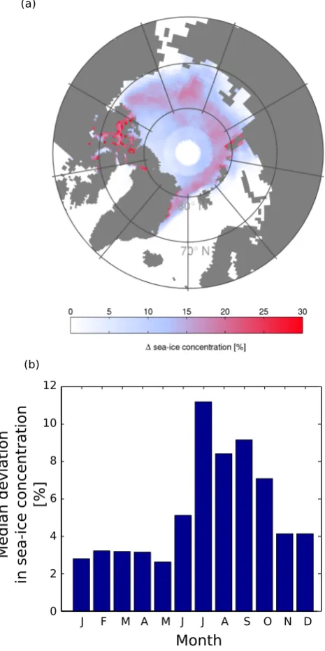
For a more detailed analysis of modelled sea-ice coverage, the regional distribution of biases must be analysed. There-fore, the mapping of differences in modelled mean sea-ice concentration is a standard tool in examining model quality. However, again the interpretation of such an analysis hinges on the reliability of the underlying concentration field as ob-tained from satellite retrievals: in particular in summer, large differences arise between different algorithms (Fig. 13a). To allow for a rough quantification of the uncertainty of re-trieved sea-ice concentration from satellite, we have calcu-lated for each month the median of the gridded difference be-tween sea-ice concentration obtained from the NASA Team algorithm and that obtained from the Bootstrap algorithm (Fig. 13b). This then allows one to estimate if a certain re-gional difference between model and satellite retrieval in a specific month still lies within the observational uncertainty. The figure confirms our analysis of the integrative measures discussed in the previous subsections: during wintertime, es-timates of sea-ice concentration are very similar for different satellite products, while a median uncertainty of around 10 % is typical for summer and early autumn. Note that this assess-ment only gives a somewhat crude estimate of the reliability of retrieved sea-ice concentration from satellites: locally, dif-ferences between the two products considered here can ex-ceed 50 % throughout the year.
J F M A M J J A S O N D
Month
12
10
8
6
4
2
0
Median
devi
a
tio
n
in
sea
-ic
e c
on
cen
tr
a
tio
n
[%
]
(b) (a)
Fig. 13. (a) Mean difference in September sea-ice concentration
be-tween Bootstrap retrieval and NASA Team retrieval for the period 1979–2007 (Bootstrap minus NASA Team). (b) Monthly median deviation in sea-ice concentration between Bootstrap retrieval and NASA Team retrieval for the period 1979–2007.
ice cover to divergent wind fields, and an assessment of the statistical distribution of sea-ice concentration as carried out as part of the present study. Through such focused analy-sis, ideally across a number of satellite algorithms, we can identify shortcomings in these algorithms and at the same time work towards identifying deficits in our sea-ice model physics.
5 Conclusions
In this paper, we have discussed how the evaluation of mod-elled sea-ice coverage against observations is affected by the incomplete knowledge of the real evolution of the sea-ice cover, by internal variability, and by technical issues such as differences in model grids. For the quantitative assessment of model quality, all these factors need to be taken into account. Our results can be summarised as following:
5.1 Evaluation of sea-ice coverage
1. Summer biases between a particular model and a par-ticular satellite retrieval can be different for sea-ice ex-tent and for sea-ice area. This is because some mod-els and some algorithms see the summer Arctic sea-ice cover as compact with a high fraction of high-concentration sea ice, while others do not. In winter, all algorithms and all models see the Arctic sea-ice cover as compact.
2. Simulations with a compact ice cover have a similar bias in sea-ice extent and in sea-ice area relative to satellite retrievals based on the Bootstrap algorithm or the ASI algorithm. Relative to these algorithms, sim-ulations with a loose ice cover with a negative bias in sea-ice extent usually have an absolute larger bias in sea-ice area, while simulations with a positive bias in sea-ice extent usually have an absolute smaller bias in sea-ice area.
3. Internal variability of sea-ice area as estimated from CMIP5 simulations is comparable to the observa-tional uncertainty as estimated from different passive-microwave algorithms, while internal variability of sea-ice extent from the simulations is about four times as large as the observational uncertainty.
4. For sea-ice area, 19 of the 26 models that we exam-ined here and for sea-ice extent, 16 of the 26 models have all their ensemble members outside of the reason-able range that we estimated from the ensemble spread from those models that capture the observed value in at least one of their ensemble members.
5. The error that is introduced in the calculation of sea-ice extent by different grid geometries can be larger than the observational uncertainty in months with a large ice coverage.
the year. The uncertainty in retrieved trends is less than 0.4 million km2decade−1 throughout the year. The median uncertainties in retrieved sea-ice concen-tration range from below 5 % throughout winter and spring to about 10 % in summer. These numbers will have to be re-assessed (and probably increased) once reliable data sets of Arctic sea-ice coverage become available that are not based on passive microwave data. 7. There is little correlation between biases in the integra-tive measures sea-ice extent and sea-ice area compared to the mean absolute bias in sea-ice concentration. This is caused by the fact that for the integrative measures, regional positive and negative biases can cancel. The average absolute bias in sea-ice concentration relative to observations is therefore a useful additional estima-tor of model quality.
5.2 Evaluation of trends
1. Internal variability of sea-ice trends as estimated from the ensemble spread of CMIP5 model simulations is so large that almost all differences in trends between observations and simulations of CMIP5 models for the period 1979–2005 (and, indeed, until 2012, see Sect. 3.5) could be caused by internal variability. Many models show in one simulation a much stronger trend than has been observed, while a different simulation with the same model and the same forcing shows for slightly different initial conditions a much weaker trend than has been observed.
2. If despite the large internal variability differences be-tween modelled and observed trends are of quantitative interest, one must note that model simulations with too fast a retreat of sea-ice extent have generally a smaller bias in simulated sea-ice-area trends relative to Boot-strap retrievals. Models that simulate too slow a retreat of sea-ice extent have generally a larger bias in sea-ice area trends. This is independent of the compactness of the ice cover.
Acknowledgements. I am very grateful to P. Griewank, A. Hau-mann, V. Kattsov, J. Marotzke, W. Meier, B. Merryfield and A. Stössel for insightful discussions and/or helpful comments on this manuscript. Comments by two reviewers were essential for improving this manuscript and are very gratefully acknowledged. I thank PCMDI for their management of CMIP5, the various modelling groups for carrying out the simulations used here, and the German Climate Computing Centre (DKRZ) whose data portal facilitated data access tremendously. NASA Team and Bootstrap algorithm sea-ice concentration data were obtained from the National Snow and Ice Data Center NSIDC, Boulder, Colorado, US. ASI Algorithm sea-ice concentration were obtained from the Integrated Climate Data Center (ICDC, http://icdc.zmaw.de/),
University of Hamburg, Hamburg, Germany. This work has been funded through a Max Planck Research-Group Fellowship.
The service charges for this open access publication have been covered by the Max Planck Society.
Edited by: D. Feltham
References
Agnew, T. and Howell, S.: The use of operational ice charts for eval-uating passive microwave ice concentration data, Atmos. Ocean, 41, 317–331, doi:10.3137/ao.410405, 2003.
Andersen, S., Tonboe, R., Kaleschke, L., Heygster, G., and Peder-sen, L. T.: Intercomparison of passive microwave sea ice concen-tration retrievals over the high-concenconcen-tration Arctic sea ice, J. Geophys. Res., 112, 18 pp., doi:10.1029/2006JC003543, 2007. Cavalieri, D. J., Gloersen, P., and Campbell, W. J.: Determination
of Sea Ice Parameters With the NIMBUS 7 SMMR, J. Geo-phys. Res., 89, 5355–5369, doi:10.1029/JD089iD04p05355, 1984.
Comiso, J. C.: Characteristics of Arctic Winter Sea Ice From Satel-lite Multispectral Microwave Observations, J. Geophys. Res., 91, 975–994, doi:10.1029/JC091iC01p00975, 1986.
Comiso, J. C. and Nishio, F.: Trends in the sea ice cover using en-hanced and compatible AMSR-E, SSM/I, and SMMR data, J. Geophys. Res., 113, C02S07, doi:10.1029/2007JC004257, 2008. Comiso, J. C., Cavalieri, D. J., Parkinson, C. L., and Gloersen, P.: Passive microwave algorithms for sea ice concentration: A com-parison of two techniques, Remote Sens. Environ., 60, 357–384, doi:10.1016/S0034-4257(96)00220-9, 1997.
Day, J. J., Hargreaves, J. C., Annan, J. D., and Abe-Ouchi, A.: Sources of multi-decadal variability in Arctic sea ice extent, En-viron. Res. Lett., 7, 034011, 2012.
Fetterer, F., Knowles, K., Meier, W., and Savoie, M.: Sea Ice In-dex, Digital media, National Snow and Ice Data Center, Boulder, Colorado USA, 2002, updated, 2012.
Kaleschke, L., Heygster, G., Lüpkes, C., Bochert, A., Hartmann, J., Haarpaintner, J., and Vihma, T.: SSM/I sea ice remote sens-ing for mesoscale ocean-atmosphere interaction analysis: Ice and icebergs, Can. J. Remote Sens., 27, 526–537, 2001.
Kay, J. E., Holland, M. M., and Jahn, A.: Inter-annual to multi-decadal Arctic sea ice extent trends in a warming world, Geo-phys. Res. Lett., 38, L15708, doi:10.1029/2011GL048008, 2011. Kwok, R.: Sea ice concentration estimates from satellite passive mi-crowave radiometry and openings from SAR ice motion, Geo-phys. Res. Lett., 29, 25-1–25-4, doi:10.1029/2002GL014787, 2002.
Massonnet, F., Fichefet, T., Goosse, H., Bitz, C. M., Philippon-Berthier, G., Holland, M. M., and Barriat, P.-Y.: Constraining projections of summer Arctic sea ice, The Cryosphere, 6, 1383– 1394, doi:10.5194/tc-6-1383-2012, 2012.
Meier, W. N.: Comparison of passive microwave ice concen-tration algorithm retrievals with AVHRR imagery, in Arc-tic peripheral seas, IEEE T. Geosci. Remote, 43, 1324–1337, doi:10.1109/TGRS.2005.846151, 2005.
CliC Arctic sea ice working group consensus document, World Climate Research Program, 2010.
Meier, W., Fetterer, F., Savoie, M., Mallory, S., Duerr, R., and Stroeve, J.: NOAA/NSIDC Climate Data Record of Passive Mi-crowave Sea Ice Concentration, Digital media, National Snow and Ice Data Center, Boulder, Colorado USA, 2011.
Notz, D. and Marotzke, J.: Observations reveal external driver for Arctic sea-ice retreat, Geophys. Res. Lett., 39, L051094, doi:10.1029/2012GL051094, 2012.
Notz, D., Haumann, A., Haak, H., Jungclaus, J., and Marotzke, J.: Arctic sea ice as simulated by MPI-ESM, J. Adv. Model. Earth Syst., 5, 173–194, doi:10.1002/jame.20016, 2013.
Parkinson, C. L., Comiso, J. C., Zwally, H. J., Cavalieri, D. J., Glo-ersen, P., and Campbell, W. J.: Arctic sea ice, 1973–1976: satel-lite passive-microwave observations, National Aeronautics and Space Administration, Washington, D.C., 1987.
Partington, K., Flynn, T., Lamb, D., Bertoia, C., and Dedrick, K.: Late twentieth century Northern Hemisphere sea-ice record from U.S. National Ice Center ice charts, J. Geophys. Res., 108, 3343, doi:10.1029/2002JC001623, 2003.
Spreen, G., Kaleschke, L., and Heygster, G.: Sea ice remote sens-ing ussens-ing AMSR-E 89-GHz channels, J. Geophys. Res, 113, C02S03, doi:10.1029/2005JC003384, 2008.
Stroeve, J., Holland, M. M., Meier, W., Scambos, T., and Serreze, M.: Arctic sea ice decline: Faster than forecast, Geophys. Res. Lett., 34, L09501, doi:10.1029/2007GL029703, 2007.
Stroeve, J. C., Kattsov, V., Barrett, A., Serreze, M., Pavlova, T., Holland, M., and Meier, W. N.: Trends in Arctic sea ice extent from CMIP5, CMIP3 and observations, Geophys. Res. Lett., 39, L16502, doi:10.1029/2012GL052676, 2012
Taylor, K. E., Stouffer, R. J., and Meehl, G. A.: An Overview of CMIP5 and the experiment design, B. Am. Meteorol. Soc., 93, 485–498, doi:10.1175/BAMS-D-11-00094.1, 2012.
Winton, M.: Do Climate Models Underestimate the Sensitivity of Northern Hemisphere Sea Ice Cover?, J. Climate, 24, 3924– 3934, doi:10.1175/2011JCLI4146.1, 2011.