© Author(s) 2014. CC Attribution 3.0 License.
Recent ice dynamic and surface mass balance of Union Glacier
in the West Antarctic Ice Sheet
A. Rivera1,2, R. Zamora1, J. A. Uribe1, R. Jaña3, and J. Oberreuter1 1Centro de Estudios Científicos, P.O. Box 5110466, Valdivia, Chile
2Departamento de Geografía, Universidad de Chile, P.O. Box 3387, Santiago, Chile 3Instituto Antártico Chileno, Punta Arenas, Chile
Correspondence to: A. Rivera ([email protected])
Received: 31 December 2013 – Published in The Cryosphere Discuss.: 20 February 2014 Revised: 22 May 2014 – Accepted: 15 June 2014 – Published: 6 August 2014
Abstract. Here we present the results of a com-prehensive glaciological investigation of Union Glacier (79°460S/83°240W) in the West Antarctic Ice Sheet (WAIS), a major outlet glacier within the Ellsworth Mountains. Union Glacier flows into the Ronne Ice Shelf, where recent mod-els have indicated the potential for significant grounding line zone (GLZ) migrations in response to changing climate and ocean conditions. To elaborate a glaciological base line that can help to evaluate the potential impact of this GLZ change scenario, we installed an array of stakes on Union Glacier in 2007. The stake network has been surveyed repeatedly for el-evation, velocity, and net surface mass balance. The region of the stake measurements is in near-equilibrium, and ice speeds are 10 to 33 m a−1. Ground-penetrating radars (GPR) have been used to map the subglacial topography, internal struc-ture, and crevasse frequency and depth along surveyed tracks in the stake site area. The bedrock in this area has a min-imum elevation of −858 m a.s.l., significantly deeper than shown by BEDMAP2 data. However, between this deeper area and the local GLZ, there is a threshold where the sub-glacial topography shows a maximum altitude of 190 m. This subglacial condition implies that an upstream migration of the GLZ will not have strong effects on Union Glacier until it passes beyond this shallow ice pinning point.
1 Introduction
WAIS, the West Antarctic Ice Sheet (Fig. 1), has been consid-ered potentially unstable because its bedrock is located well below sea level (Bamber et al., 2009) and its total disinte-gration could contribute up to 4.3 m (Fretwell et al., 2013) to
Figure 1. Left: WAIS location map. Right: Union Glacier basin (light-blue area). In yellow, the main ice divides in the region. In dashed
white the 2005 track to subglacial Lake Ellsworth (517 km). In green, the new track surveyed in 2010 (235 km). Stakes B1 to B9 are described in the text. The black box is shown in Fig. 2. Background image: MODIS Mosaic of Antarctica (MOA: Scambos et al., 2007).
to retreat of the GLZ. This, in turn, would favour higher ice fluxes along tributary glaciers, and thinning that will spread upstream along deep channels (Rignot et al., 2011b).
Between two of the main ice streams in the region (Rut-ford and Institute), there are two smaller glaciers also drain-ing into the RnIS: Union Glacier (79°460S/83°240W) flow-ing into Constellation Inlet, and the Horseshoe Valley glacier (80°180S/81°220W) flowing into Hercules Inlet. The study of these glaciers could provide an important clue about ongo-ing changes takongo-ing place in the region, especially considerongo-ing that local glacier mass balance can be significantly affected by RnIS changes.
In this context, the main aim of this paper is to present recent glaciological results obtained at Union Glacier and nearby areas that provide a base line for possible ice dynamic responses to ongoing and modelled future changes of RnIS.
2 Study area
Union Glacier (79°460S/83°240W) (Fig. 2) has an estimated
total area of 2561 km2, with a total length of 86 km from the ice divide with the Institute Ice Stream down to the ground-ing line of Constellation Inlet on the RnIS. The glacier has several glacier tributaries, the main trunks being located in the Union and Schanz valleys (Figs. 1 and 2), which are fed through narrow glacial valleys (9 km wide) flowing from the interior plateau until they merge at the Union “gate”. This gate or narrowest section of the glacier (7 km wide) has a me-dial moraine line comprised of clasts and small-sized debris.
The local Union Glacier blue ice area (BIA) is used for landing Ilyushin IL76 airplanes on wheels under a contract with the private company Antarctic Logistics and Expedi-tions (ALE) llc. This company has been operating in the region since the 1980s, when they began to use the Pa-triot Hills BIA (Wendt et al., 2009) at Horseshoe Valley (80°180S/81°220W) for landing heavy airplanes. However, these airplane operations were frequently disrupted due to strong prevailing cross winds at Patriot Hills. In order to increase the number of airplane operational days and to improve access for heavy cargo airplanes, in 2007/8 ALE moved to Union Glacier, where the prevailing wind direction is in line with the landing strip (katabatic winds), helping air-planes to operate even with strong gusts. Thanks to ALE lo-gistic support, four scientific campaigns have been conducted on Union Glacier since 2008, where a glaciological program was established, including ice dynamics, mass balance and geophysical surveys (Rivera et al., 2010).
Figure 2. Yellow dots show the stakes described in the text (Fig. 1 and Table 2). RX1 is the location of the static GPS on rock. Crevasses
are shown in red. The Union Glacier “gate” is a transversal profile between B18 and B15 (inset) where the ice runway is shown in purple. Mean ice velocity area shown as arrows. Summer base camp is visible near B11. The background image is an ASTER false composite 321 acquired on 1 February 2013. Upper right: predominant wind speed and direction for 2008–2012 at the Union Glacier automatic weather station, installed near stake V17.
3 Methods
3.1 Meteorological data
The meteorological data analysed here were collected at the Union Glacier automatic weather station (AWS) installed near stake V17, which has been operating since 2008 (Fig. 2). The AWS data series show several data gaps due to malfunc-tion or low power supply problems during the winter. In spite of these, the available data are good enough for weather fore-casts during landing operations in the summer, and for de-scribing general temperature conditions in the area as well as predominant winds and directions.
3.2 Remote sensing
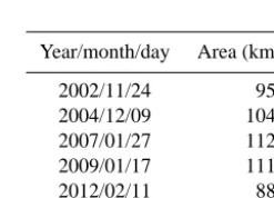
Mid-summer ASTER satellite images acquired between 2002 and 2013 (Table 1) were analysed and classified via manual digitalisation in order to delineate the local Union
Table 1. BIA extension based upon ASTER images collected since
2002.
Year/month/day Area (km2)
2002/11/24 95.6
2004/12/09 104.7 2007/01/27 112.0 2009/01/17 111.8
2012/02/11 88.2
2013/02/01 96.7
Glacier main BIA. This task allowed areal changes in snow cover to be quantified and analysed for possible relationships with local meteorological data.
the contrast and brightness modified by means of histogram equalisation to facilitate the delimitation of the blue ice area. The BIA outline mapping was based upon a similar pro-cedure established by Rivera et al. (2014), where the bound-ary between snow and ice is identified manually assuming the maximum extent criterion of identification. This is eas-ily done thanks to the spectral differences between snow and ice.
3.3 Glaciological mass balance
Stake heights above the snow/ice surface were measured yearly between 2007 and 2011 (Figs. 1 and 2; Table 2). Of 88 potential stake measurements at the gate, 72 were acquired successfully. The annual heights were compared and local mass balance was subsequently calculated. In order to con-vert these values into their water equivalent, a mean density of 910 kg m−3 (Paterson, 1994) was used for stakes drilled on ice. In those cases where the stakes were located at snow surfaces, the densities were measured by using a Mount Rose snow probe with a penetration capacity of near 50 cm of snow firn. The snow density accuracy obtained by the use of this device is estimated to be near 12 % (Conger and McClung, 2009).
3.4 GPS
In December 2007, the initial observation network of 21 bamboo stakes was installed in a BIA on Union Glacier (Fig. 2). For each of these stakes GPS measurements were made using Topcon GR3 dual-frequency GPS receivers with measurement times of less than 30 s per stake, yielding metre-scale errors. In December 2008, 2009 and 2010, the same network as well as 35 new stakes were surveyed with dual-frequency Javad GPS model Lexon GGD receivers. In order to apply a differential correction procedure, a similar GPS receiver continuously collected data at a rock location (RX1 in Fig. 2). The precision obtained by these surveys improved to less than 10 cm by measuring between 15 and 30 min per stake. In addition, a dual-frequency Javad GPS receiver was installed on snow (Bstat in Fig. 2), collecting data between 11 December 2009 and 31 January 2010 for high-resolution studies (every 30 s), with the aim of detecting possible tidally modulated ice velocities. In January 2011, a real-time kinematic procedure was applied to data collected at the Union Glacier gate by a Leica SR 9500 receiver, with estimated decimetre accuracy. All GPS data collected were processed using the GrafNav 8.20 commercial software. 3.5 Surface elevation changes and geodetic mass
balance estimation
The data obtained by the GPS measurements were compared in order to calculate the local mass balance and the absolute surface elevation changes in the BIA.
Using the measured height differences obtained by GPS and considering the surface topographic slope effect, the sub-mergence/emergence velocity (we) was calculated:
we=ws−ustanα, (1)
wherews is the vertical ice velocity, us is the ice velocity along the surface flow direction andαis the slope. The emer-gence velocity represents the vertical flow of ice relative to the glacier surface and allows the estimation of the net bal-ance if it is assumed that density does not change with depth during the period (Hooke, 2005).
By subtracting the emergence velocity of the measured specific balance (stake height difference), the surface eleva-tion change with time at a fixed posieleva-tion can be obtained.
∂h
∂t =b−we (2)
If the glacier is in a steady state, there would be no surface changes, since accumulation and ablation compensate for the submergence and emergence velocities, so that the sur-face profile remains unchanged (Hooke, 2005). In this case
b=we; however, most glaciers are not perfectly in steady state. Only the stake array measured at the Union gate was considered for this analysis.
3.6 Radar
A Coherent pulse compression radar depth sounder designed at Centro de Estudios Científicos CECs (Uribe et al., 2014) was used to measure ice thickness. The radar operates at a central frequency of 155 MHz, a maximum of 10 kHz of pulse repetition frequency (PRF), a bandwidth of 20 MHz and peak power of 200 W. Yagi antennae were used for both the transmitter and the receiver. We use two channels for si-multaneous low and high signal amplification to increase the dynamic range of this radar.
A frequency-modulated continuous-wave (FM-CW) radar also designed by Uribe et al. (2014) was used to measure sur-face snow and ice layering to a depth of 450 m with a high vertical resolution (1 m). This radar works at a frequency from 550 to 900 MHz using two separated log periodic anten-nae for the transmitter and receiver. The transmit power was 21 dBm, and the whole system operated at a PRF of 10 kHz. A direct digital synthesis (DDS) system was used to generate an extremely linear frequency sweep transmitted signal.
Table 2. Stake co-ordinates, velocities and mass balance per period. See Figs. 1 and 2 for locations.
Stakes Lat.° Lon.° H. Velocity Mass balance Period Type of surface (m a e) (m a−1) (m w.eq. a−1)
B1 −80.211 −81.230 803.12 12.7 0.18
2008–2009
Snow
B2 −80.124 −81.113 813.51 1.8 0.19
B3 −80.045 −80.937 759.07 0.6 0.04
B4 −79.985 −81.080 573.57 1.8 0.06
B5 −79.922 −81.211 538.16 2.0 −0.07 Snow/BIA
B6 −79.840 −81.298 669.59 0.1 0.03
Snow
B7 −79.801 −81.348 553.87 1.2 0.04
B8 −79.757 −81.965 459.99 2.9 0.14
B9 −79.709 −82.455 531.04 33.3 0.14
Bstat −79.708 −82.454 531.34 33.0 – 2009/11/12 2010/31/01
B10 −79.717 −82.643 639.79 34.6 0.17
2008–2009 B11 −79.757 −82.803 672.46 20.5 0.13
B12 −79.760 −82.931 690.56 20.9 0.20
B13 −79.764 −83.091 703.53 22.9 −0.09
Ice B14 −79.768 −83.266 738.39 22.4 −0.06
B15 −79.798 −83.281 735.19 21.6 −0.16 B16 −79.796 −83.316 742.20 23.2 −0.13
B17 −79.765 −83.343 739.36 17.0 −0.08
Ice/crevasses B18 −79.760 −83.370 747.68 14.0 −0.11
B19 −79.764 −83.372 743.72 11.1 −0.10
V00 −79.769 −83.370 739.47 18.1 −0.08 2008–2010
Ice V01 −79.770 −83.370 738.44 19.0 −0.08 2007–2011
V02 −79.772 −83.368 738.13 20.2 −0.04 2007–2010
V03 −79.774 −83.365 739.69 21.7 −0.11
2007–2011 V04 −79.775 −83.363 736.40 22.3 −0.07
V05 −79.777 −83.361 733.57 23.0 −0.22
V06 −79.779 −83.358 735.12 23.5 −0.11
2007–2010 V07 −79.781 −83.355 736.61 23.9 −0.08
V08 −79.784 −83.352 739.05 24.3 −0.13 2007–2009
V09 −79.787 −83.343 738.60 24.3 −0.11
2007–2011 V10 −79.790 −83.334 737.63 24.3 −0.13
V11 −79.792 −83.325 738.82 24.0 −0.07 2007–2010
V12 −79.771 −83.337 738.51 21.9 −0.09
2007–2011 V13 −79.773 −83.335 735.87 22.3 −0.08
V14 −79.774 −83.332 733.20 22.4 −0.08 V15 −79.777 −83.327 731.27 22.7 −0.09
V16 −79.779 −83.323 731.72 23.1 −0.10 2007–2009
V17 −79.782 −83.316 731.16 23.4 −0.11
2007–2011 V18 −79.784 −83.313 730.33 23.5 −0.13
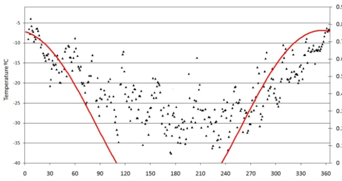
Figure 3. Mean daily temperature (°C) during 2008 (black triangles) and modelled solar direct radiation (red line) at the AWS site (kWm−2).
alert the driver of the presence of hyperbolae potentially re-lated to crevasses.
Post-processing and data analyses were carried out us-ing Reflex-Win V5.6 (Sandmeier Scientific Software) for the three radar systems. Background removal, a dewow filter and adjustment of the gain function, among other procedures, were applied to the raw data. For crevasse analysis, migra-tion correcmigra-tion procedures were also applied to collapse the hyperbolic diffractions to their proper point origins (Plewes and Hubbard, 2001). In order to convert travel time to ice thickness in metres, it was assumed that the electromag-netic wave travelled through the ice at 0.168 m ns−1, a mean value representative of cold ice (Glen and Paren, 1975), and at 0.194 m ns−1 assumed to be representative of snow/firn (Woodward and King, 2009).
4 Results
4.1 Meteorological data and BIA area changes
The meteorological data collected at Union Glacier between 2008 and 2013 contain several gaps and invalid records, but in general provide a good idea of the local conditions, which are especially useful for landing operations. In terms of cli-matological analysis, the series is too short and noisy, but is the only one available in the region.
The mean daily air temperature at this location (Fig. 3) from 2008 to 2012 was−20.6 °C, with an absolute minimum of−42.7 °C recorded on 12 August 2008 at 2 a.m. and an ab-solute maximum of 0.5 °C registered on 15 January 2010 at 8 p.m. Daily air temperatures have maximums in December– January following direct solar radiation; however, between April and August (included), when the Sun is below the hori-zon, the lowest temperatures have a mean of−25.5±3.5 °C. Temperatures close to the melting point have only been
ob-served in three summer events: 7–8 January 2008, 14–15 Jan-uary 2010 and 25–26 December 2010, but no surface melting has been observed on this site. The mean air temperature in January is−10.3 °C.
Regarding wind speed and direction, the data are very consistent between 2008 and 2012, with a mean value of 16.3 knots and a predominant direction from 224°. The max-imum wind speed recorded on site was near 60 knots and the predominant wind speeds are higher than 25 knots (Fig. 2). This predominant wind direction explains the extension of the main BIA, which experienced less than 10 % area change between 2002 and 2013. The available scene dates show some expected seasonal variability, especially when com-paring more stable midsummer scenes (December–January) with early or late summer scenes (Brown and Scambos, 2005). The series is however too short to detect a trend (Ta-ble 1).
4.2 Surface mass balance
Snow densities measured at stakes drilled on snow surfaces have a mean value of 400±3 kg m−3, with low variability between all surveyed stakes. No fresh and soft snow was de-tected due to the lack of precipitation in the region during our surveys. Table 2 indicates the details of each stake, the type of surface and the period of the measurements.
The surface mass balance estimations between 2007 and 2011 at the stakes installed on the BIA gate (V00 to V21, Table 2) are typically negative (Fig. 4), with a mean inter-annual surface mass balance of−0.097 m w.eq. a−1.
Figure 4. Mass balance (m w.eq. a−1) for 2007–2011 at stakes located at the local BIA. Stake locations are shown in Fig. 2.
Figure 5. Ice velocities (m a−1) at the Union Glacier gate by indicated years. Stake locations are shown in Fig. 2.
of 0.3 m a−1(0.12 m w.eq. a−1). Just outside the BIA, stake B12 showed the maximum net balance (0.2 m w.eq. a−1), in-dicating that snow drift coming from the BIA due to the predominant katabatic wind direction (Fig. 2) is having a positive downstream accumulation effect. The only negative surface mass balance along the Patriot Hills–Union Glacier track (excluding the Union Glacier BIA) was detected at stake B5, which is located at the edge of the local BIA of the Plumber glacier (Fig. 1). Here a modest −0.07 m w.eq. a−1 (Table 2) was obtained between 2008 and 2009. Stakes B13– B19 (Table 2, Fig. 2) also had negative values, with a mean surface balance of 0.1 m w.eq. a−1, coincident with the other stakes located at a local BIA.
4.3 Surface ice velocity
Surface ice velocities were obtained for 19 stakes (B1–B19) located along the track between Patriot Hills and the Union Glacier base camp (Figs. 1 and 2), with measurement
peri-ods of nearly 1 yr, and resulting ice velocities between 0.1 and 34.6 m a−1(Table 2). Minimum values were observed at local ice divides (B2–B8), while the maximum velocity was observed at stake B10 located in the steepest area of Union Glacier, between two crevasse fields (Fig. 2).
H. Gudmunsson (personal communication, 2010), no tidal effect was detected.
The neighbouring stake of Bstat (B9, located within a dis-tance of 10 m) was only measured for 30 min in December 2009 and in December 2010, resulting in an annual veloc-ity of 33.26±0.7 m a−1. The good correspondence with the Bstat results (33 m a−1) indicates that Union Glacier does not show important seasonal ice velocity changes.
At the Union Glacier gate stake array (Fig. 2), 22 stakes were drilled into its blue ice area in 2007 and were resur-veyed annually until 2011. Unfortunately, not all the original stakes have survived or were re-measured every year. How-ever, from the remaining stake network a mean velocity of 20 m a−1was estimated for the measurement period (Fig. 5). The overall ice motion at the gate is similar to the main wind direction (Fig. 2) observed in the BIA. No temporal velocity changes were observed during the studied period.
4.4 Surface elevation change
Considering the surface velocities obtained for the stakes (Table 2), and by applying Eq. (1), a mean vertical veloc-ity for the blue ice of−0.07±0.007 m a−1was found at the Union Glacier gate. For a steady-state glacier this would be equal to the local mass balance; however, this is not the case for the studied area (there is a negative mass balance in the BIA), and a mean local elevation change of −0.012 m a−1 was found. In any case, this result is close to the estimated er-ror of the measurements and indicates near-equilibrium con-ditions.
4.5 Glacier thickness and internal structure
More than 450 km of radar tracks were measured between 2008 and 2010 in the Union Glacier area, including oversnow traverses between Patriot Hills, Union Glacier and the high Antarctic plateau.
The 80 km long profile between the Antarctic plateau and Union Glacier (Fig. 6 upper), including the transit along the Balish, Schneider, Schanz and Driscoll glaciers, was sur-veyed with a FM-CW radar for snow accumulation data, a compression pulse radar for ice thickness data and a GPR system for crevasse detection purposes.
The deep ice of the plateau is seen at the beginning of the survey profile (A in Fig. 6), and is then followed by a pas-sage characterised by shallow ice (B) where the steepest sec-tion of the whole traverse was crossed. After this secsec-tion, the thickness increases sharply until a local maximum thickness of 1120 m was observed at Balish Glacier. The local divide between the Balish and Schneider glaciers (C in Fig. 6) has a prominent subglacial peak (C in Fig. 6) where the moun-tain range dividing the two glaciers is also visible under-neath the ice. The maximum thickness measured at Schnei-der Glacier was 900 m, 1050 m at Schanz Glacier, 1510 m at Driscoll Glacier and 1540 m at Union Glacier, close to
the base camp. The mean ice thickness measured at Union Glacier was 1450 m. The subglacial topography in the valley is smooth, with “U”-shaped flanks.
At the beginning of the radar profile (A–B in Fig. 6), it is possible to see the shallowest ice at the Gifford Peaks pass (passage), with a thickness between 45 and 140 m obtained by the low-gain channel of the pulse compression radar. This profile is not visible in the high-gain channel, due to set-up constraints on this system (Uribe et al., 2014).
The FM-CW radar detected multiple internal snow–firn layers and the snow–ice boundary layer with a high resolu-tion. Figure 7 shows an FM-CW profile at Union Glacier, where the snow–ice boundary layer is at a depth of 30–40 m (between A and B in Fig. 7) and then tends to disappear when approaching the BIA (between C and D in Fig. 7). The cen-tral moraine line of the glacier is indicated by the letter C in Fig. 7.
The GPR data collected along the track from Union Glacier to the Antarctic plateau allowed the detection of many crevasses both near the runway area and at the Gif-ford Peaks passage, just before reaching the plateau. Along the survey route the GPR system was able to detect the up-per 20 m of the internal structure of the ice. Within this upup-per layer, annual snow/firn layers suffered (in places) disconti-nuities due to crevasses that appeared as hyperbolae on the radar traces.
In general, the route from Union Glacier to the Antarc-tic plateau is almost totally free of crevasses. An exception to this was the Gifford passage (B in Fig. 6), where a mi-nor system of crevasses was detected, with widths between 1 and 5 m and snow bridges between 1.5 and 3 m thick. In spite of these crevasses, the Gifford passage is the shortest (235 km) gateway for oversnow traverses from Union Glacier to the Subglacial Lake Ellsworth (Vaughan et al., 2007) on the Antarctic plateau. The alternative route to this subglacial lake is nearly 520 km long, starting at Union Glacier, passing along Patriot Hills, then travelling around the Three Sails and finally turning west toward the Subglacial Lake Ellsworth (Fig. 1).
5 Discussion
Figure 6. Top: location map of the radar and GPS survey measured between the Antarctic Plateau (A) and Union Glacier (F) in 2010 (green
line). In blue, the available data between F and the local grounding line zone (in red, from Rignot et al., 2011a) at Constellation Inlet (G). The background image is the RAMP AMM-1 SAR Image Mosaic of Antarctica (Jezek and RAMP Product Team, 2002). Bottom: surface (red line) and subglacial topography (blue line) interpreted from the radar data collected in 2010 along the A–F track.
In spite of this negative surface mass balance, the result-ing ice elevation changes between 2008 and 2011 at the Union gate are very close to the error of the measurements (combined error of 0.01 m), with a mean of −0.012 m a−1 and high spatial variability (±0.044 m a−1) among the gate stakes. Accordingly, the glacier must be considered in equi-librium, without significant changes compared with previous data (Rivera et al., 2010).
The ice velocities at the BIA fluctuate between 11 and 24 m a−1, without significant changes between 2007 and 2011. However, downstream of the Union gate, the velocities
increase up to 33 m a−1at the continuous GPS stake (Bstat), where no seasonal variations or tidally modulated variability were detected.
Figure 7. FM-CW data obtained at Union Glacier. Top: location of the surveyed track near the base camp of Union Glacier. The background
image is an ASTER false composite 321 acquired on 14 March 2013. Bottom: radargram showing the surface topography (red line), internal annual snow/firn layers and the firn/ice boundary (blue line). Letters A and B indicate the base camp where the snow/firn layers are near 30–40 m thickness in total. Letter C corresponds to the medial moraine line of the glacier. Letter D indicates the appearance of the BIA at the surface.
thicknesses (less than 1 m), its resolution being insufficient to detect the first metres of the snow pack.
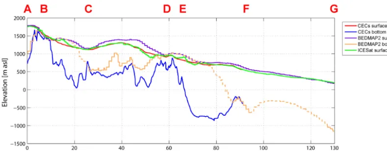
Comparisons of surface and bedrock topography along transect A–F (Fig. 8) resulted in a maximum ice thickness difference of 1447 m, with a mean difference of 477 m (stan-dard deviation 348 m) between the data presented here and BEDMAP2 (Fretwell et al., 2013). The surface topography of the surveyed traverse was found to differ from BEDMAP2 and ICESat (2003–2005) by means of 91 and 169 m, respec-tively. These differences are understandable due to the coarse resolution of BEDMAP2 and the footprint of ICESat.
The subglacial topography (Fig. 8) at the main trunk of Union Glacier toward the local GLZ (Segment E–G in Fig. 6) showed a subglacial topography well below sea level (near −858 m), much deeper than previously estimated by BEDMAP2. However, between Union Glacier and the local GLZ, the subglacial topography shows a maximum altitude of−190 m at F in Figs. 6 and 8. The subglacial topography then deepens toward the GLZ, where the bedrock is esti-mated to be 1050 m below sea level (Fretwell et al., 2013).
This subglacial condition implies that an upstream migration of the GLZ until point F in Figs. 6 and 8 will not have a strong effect on Union Glacier. However, the glacier can respond in a more dynamic way if this possible migration affects Union Glacier upstream of this potential pinning point.
6 Conclusions
Figure 8. Comparisons of surface and bedrock topography of different data sources along transect A–G (see the upper panel of Fig. 6 for the
location of the transect). CEC surface and bedrock from the year 2010. ICESat surface from 2003 to 2005, BEDMAP2 surface and bedrock from Fretwell et al. (2013). The BEDMAP2 bottom dashed line is interpolated.
Ice dynamics were also recorded thanks to the measure-ment of ice velocities and ice thicknesses. Maximum ice ve-locity values of 34.6 m a−1were obtained. Near-equilibrium conditions were calculated at the BIA, where mean velocities of 20 m a−1were measured. The snow accumulation among the studied stakes outside the BIA showed values of up to 0.2 m w.eq. a−1(near 0.5 m a−1of snow). At the BIA, a local negative mass balance was detected as expected, with mean ablation rates of 0.1 m w.eq. a−1.
Due to the below sea level subglacial topography upstream of the local GLZ, it is expected that Union Glacier can expe-rience some thinning and acceleration in future scenarios of GLZ migration. However, these impacts will not affect the whole glacier, because at near 55 km upstream of the present GLZ, the bedrock topography has a prominent ridge perpen-dicular to the main ice flow direction, where the bedrock has a maximum altitude of−190 m a.s.l. This ridge can play an important role in modulating future glacier responses by en-abling the grounding line to come to a prolonged standstill, providing the glacier with a “pinning point”.
Overall, the collected data allowed a ground route from Union Glacier to the upper Antarctic plateau to be mapped satisfactorily. The route is important, as it traverses the Subglacial Lake Ellsworth and the main ice streams flow-ing into the Amundsen Sea Embayment area (Pine Island Glacier) and toward the Weddell Sea (Institute and Rutford ice streams). This new 235 km long route toward the Sub-glacial Lake Ellsworth is shorter than half of the previously traversed track of 517 km, providing a much more direct and shorter gateway to inner Antarctica.
Acknowledgements. This research was supported by Antarctic Logistic Expeditions (ALE) Ltd. Special thanks to M. Sharp, P. Mc-Dowell, C. Jacobs, Eddy, Boris and all ALE personnel at Union Glacier. CECs is funded by the Basal fund of CONICYT, among other grants. J. A. Neto collaborated with GPS data collection in
2011. A. Wendt, C. Rada, T. Kohoutek and M. Barandun helped with data processing. H. Gudmundsson analysed the GPS data at Bstat in order to detect possible tidally modulated effects on the ice flow. J. Carrasco and F. Burger helped with the met data. D. Carrión helped with figures and satellite image analysis. R. Wilson edited the text. The GLIMS project provided ASTER data. A. Rivera is a Guggenheim fellow. The comments and suggestions by Ted Scambos and Neil Ross are highly appreciated.
Edited by: E. Larour
References
Bamber, J., Riva, R., Vermeersen, B., and LeBrocq, A.: Reassess-ment of the potential. Sea-level rise from a collapse of the West Antarctic Ice Sheet Science, Science, 324, 901–903, 2009. Brown, I. and Scambos, T.: Satellite monitoring of blue ice extent
near Byrd Glacier, Antarctica, Ann. Glaciol., 39, 223–230, 2005. Carrasco, J., Casassa, G., and Rivera, A.: A warm event at Patriot Hills, Antarctica: An ENSO related phenomena?, in: Sixth Inter-national Conference on Southern Hemisphere Meteorology and Oceanography, 240–241, Santiago, Chile, 2000.
Cavalieri, D. and Parkinson, C.: Antarctic sea ice variabil-ity and trends, 1979–2006, J. Geophys. Res., 113, C07004, doi:10.1029/2007JC004564, 2008.
Conger, S. and McClung, D.: Comparison of density cutters for snow profile observations, J. Glaciol., 55, 163–169, 2009. Fretwell, P., Pritchard, H., Vaughan, D., Bamber, J., Barrand, N.,
Welch, B., Wilson, D., Young, D., Xiangbin, C., and Zirizzotti, A.: Bedmap2: improved ice bed, surface and thickness datasets for Antarctica, The Cryosphere, 7, 375–393, doi:10.5194/tc-7-375-2013, 2013.
Glen, J. and Paren, J.: The electrical properties of snow and ice, J. Glaciol., 15, 15–38, 1975.
Gudmundsson, G.: Fortnightly variations in the flow velocity of Rutford Ice Stream, West Antarctica, Nature, 444, 1063–1064, 2006.
Hellmer, H., Kauker, F., Timmermann, R., Determann, J., and Rae, J.: Twenty “first” century warming of a large Antarctic ice-shelf cavity by a redirected coastal current, Nature, 485, 225–228, 2012.
Hooke, R.: Principles of Glacier Mechanics, Cambridge University Press, Cambdridge, UK, 2nd edn., 2005.
Jezek, K. and RAMP Product Team: RAMP AMM-1 SAR Image Mosaic of Antarctica. Version 2. Fairbanks, AK: Alaska Satel-lite Facility, in association with the National Snow and Ice Data Center, Boulder, CO. Digital media, 2002.
Joughin, I. and Bamber, J.: Thickening of the ice stream catchments feeding the Filchner-Ronne Ice Shelf, Antarctica, Geophys. Res. Lett., 32, L17503, doi:10.1029/2005GL023844, 2005.
Mayewski, P., Meredith, M., Summerhayes, C., Turner, J., Worby, A., Barrett, P., Casassa, G., Bertler, N., Bracegirdle, T., Naveira, A., Bromwich, D., Campbell, H., Hamilton, G., Lyons, W., Maasch, K., Aoki, S., Xiao, C., and van Ommen, T.: State of the Antarctic and Southern Ocean climate system, Review of Geo-physics, 47, RG1003, doi:10.1029/2007RG000231, 2009. Paterson, W.: The physics of glaciers, Pergamon Press, Great
Britain, 3rd edn., 1994.
Plewes, A. and Hubbard, B.: A review of the use of radio-echo sounding in glaciology, Prog. Phys. Geog., 25, 203–236, 2001. Rignot, E. and Jacobs, S.: Rapid bottom melting widespread near
Antarctic Ice Sheet grounding lines, Science, 296, 2020–2023, 2002.
Rignot, E. and Thomas, R.: Mass balance of polar ice sheets, Sci-ence, 297, 1502–1506, 2002.
Rignot, E., Vaughan, D., Schmeltz, M., Dupont, T., and MacAyeal, D.: Acceleration of Pine Island and Thwaites Glaciers, West Antarctica, Ann. Glaciol., 34, 189–194, 2002.
Rignot, E., Mouginot, J., and Scheuchl, B.: Antarctic ground-ing line mappground-ing from differential satellite radar interferometry, Geophys. Res. Lett., 38, L10504, doi:10.1029/2011GL047109, 2011a.
Rignot, E., Mouginot, J., and Scheuchl, B.: Ice Flow of the Antarctic Ice Sheet, Science, 333, 1427–1430, 2011b.
Rivera, A., Zamora, R., Rada, C., Walton, J., and Proctor, S.: Glacio-logical investigations on Union Glacier, Ellsworth Mountains, West Antarctica, Ann. Glaciol., 51, 91–96, 2010.
Rivera, A., Cawkwell, F., Wendt, A., and Zamora, R.: Map-ping Blue Ice Areas and Crevasses in West Antarctica Using ASTER Images, GPS and Radar Measurements, in: Global Land Ice Measurements from Space, edited by: Kargel, J., Leonard, G., Bishop, M., Kääb, A., and Raup, B., chap. 31, 743–757, Springer-Praxis, Heidelberg, 2014.
Ross, N., Bingham, Corr, H., Ferraccioli, F., Jordan, T., Le Brocq, A., Rippin, D., Young, D., Blankenship, D., and Siegert, J.: Steep reverse bed slope at the grounding line of the Weddell Sea sector in West Antarctica, Nat. Geosci., 5, 393–396, 2012.
Scambos, T., Haran, T., Fahnestock, M., Painter, T., and Boh-lander, J.: MODIS-based Mosaic of Antarctica (MOA) data sets: continent-wide surface morphology and snow grain size, Remote Sens. Environ., 111, 242–257, 2007.
Uribe, J., Zamora, R., Gacitúa, G., Rivera, A., and Ulloa, D.: A low power consumption radar system for measuring ice thickness and snow/firn accumulation in Antarctica, Ann. Glaciol., 55, 39–48, 2014.
Vaughan, D., Rivera, A., Woodward, J., Corr, H., Wendt, J., and Zamora, R.: Topographic and hydrological controls on Sub-glacial Lake Ellsworth, West Antarctica, Geophys. Res. Lett., 34, L18501, doi:10.1029/2007GL030769, 2007.
Wendt, A., Casassa, G., Rivera, A., and Wendt, J.: Reassessment of ice mass balance at Horseshoe Valley, Antarctica, Antarct. Sci., 21, 505–513, 2009.