Atmos. Meas. Tech., 5, 1637–1651, 2012 www.atmos-meas-tech.net/5/1637/2012/ doi:10.5194/amt-5-1637-2012
© Author(s) 2012. CC Attribution 3.0 License.
Atmospheric
Measurement
Techniques
Consistency between Fourier transform and small-volume few-wave
decomposition for spectral and spatial variability of gravity waves
above a typhoon
C. I. Lehmann1, Y.-H. Kim2, P. Preusse1, H.-Y. Chun2, M. Ern1, and S.-Y. Kim2,3
1Institut f¨ur Energie- und Klimaforschung (IEK-7), Forschungszentrum J¨ulich, J¨ulich, Germany 2Department of Atmospheric Sciences, Yonsei University, Seoul, South Korea
3Next Generation Model Development Center, Seoul, South Korea Correspondence to: C. I. Lehmann ([email protected])
Received: 18 January 2012 – Published in Atmos. Meas. Tech. Discuss.: 20 February 2012 Revised: 12 June 2012 – Accepted: 18 June 2012 – Published: 17 July 2012
Abstract. Convective gravity wave (GW) sources are spa-tially localized and emit at the same time waves with a wide spectrum of phase speeds. Any wave analysis there-fore compromises between spectral and spatial resolution. Future satellite borne limb imagers will for a first time pro-vide real 3-D volumes of observations. These volumes will be however limited which will impose further constraints on the analysis technique. In this study a three dimensional few-wave approach fitting sinusoidal few-waves to limited 3-D vol-umes is introduced. The method is applied to simulated GWs above typhoon Ewiniar and GW momentum flux is estimated from temperature fluctuations. Phase speed spectra as well as average profiles of positive, negative and net momentum fluxes are compared to momentum flux estimated by Fourier transform as well as spatial averaging of wind fluctuations. The results agree within 10–20 %. The few-wave method can also reveal the spatial orientation of the GWs with respect to the source. The relevance of the results for different types of measurements as well as its applicability to model data is discussed.
1 Introduction
Gravity waves (GWs) are atmospheric waves conveying mo-mentum and energy from the lower into the mid and upper atmosphere. They are the main driver of the mesospheric cir-culation and the main reason for the cold summer mesopause (e.g. McLandress, 1998) and contribute 50 % or more to
the driving of the QBO (Dunkerton, 1997; Ern and Preusse, 2009; Alexander and Ortland, 2010). Climate modeling in-dicates that they provide a significant portion of the pdicted acceleration of the Brewer-Dobson circulation in re-sponse to CO2 increase (McLandress and Shepherd, 2009; Butchart et al., 2010). These and many other effects make GWs to be one of the most important coupling processes in the atmosphere.
The acceleration or deceleration of the background wind (frequently called GW drag) is given by the vertical gradient of the pseudomomentum flux (Fritts and Alexander, 2003). This gradient is caused, in general, by GW dissipation and is particularly strong below a critical level where the phase speed of the wave matches the background wind speed. In order to understand the interaction of GWs with the back-ground wind, one, therefore, has to determine both the spa-tial distribution of GW sources and the phase speed distribu-tion of pseudomomentum flux associated with these sources (Preusse et al., 2006; Alexander et al., 2010).
The vertical flux of horizontal pseudomomentum associ-ated with a GW is given by (Fritts and Alexander, 2003)
Fpx, Fpy
= 1− f
2
ˆ
ω2
!
¯
ρu0w0, v0w0 (1)
wave periods or one or several full wavelengths. However, measurements may not have access to these quantities and therefore equivalent expressions are deduced based on the dispersion relation and polarization relations. For instance, satellite-borne infrared emission sounders can measure snap-shots of temperatures. As shown by Ern et al. (2004), the pseudomomentum flux then can be calculated from the tem-perature amplitudesTˆand the three-dimensional wave vector (k,l,m) by
Fpx, Fpy =
1 2ρ¯
(k, l) m
g N
2 Tˆ
¯
T !2
. (2)
N is the buoyancy frequency,gthe gravity acceleration,ρ¯
the background atmosphere density andT¯ the background atmosphere temperature. Spectral properties of the wave are therefore not only important for the interpretation, but also essential to determine the pseudomomentum flux, in particu-lar from temperature measurements.
To determine the spectral wave parameters is a challenging task. Gravity waves are highly intermittent and maxima in momentum flux are located close to the sources. Over small distances momentum flux may vary 1–2 orders of magni-tude. For instance, only 1 horizontal wavelength upwind of a mountain range, GW momentum flux is often almost neg-ligibly small. On the other hand, the wave spectrum consists of a superposition of a number of wave components. Any method for analyzing GWs therefore is necessarily a com-promise between spectral and spatial resolution. In addition, different data sets and, in particular, measured data provide additional limitations.
Fourier transform is a mathematically well-founded method for the analysis of regularly gridded model data. The underlying assumptions are periodicity as well as spa-tial homogeneity and temporal stationarity of the data. Ho-mogeneity means that all spatial variations are explained in terms of the superposition of waves, i.e. all wave compo-nents are present in all regions of the analyzed volume with the same amplitude. In this view, regions of higher or lower variance express a constructive or destructive interference of the waves. Stationarity is the temporal analogue. This is an approximation which is not fully consistent with our under-standing of localized GW sources.
According to the Parseval theorem, the Fourier compo-nents are linked to the variance. Therefore, the net momen-tum flux (i.e. the sum of all negative and positive compo-nents) calculated from the whole spectrum is mathematically equivalent to the net momentum flux calculated directly from the wind variance. However wind fluctuations due to gravity waves are difficult to measure. In particular, direct estimation from horizontal and vertical wind variances cannot be ap-plied to many atmospheric measurements (e.g. satellite data and radiosondes) and do not provide insight in the spectral properties.
New detector technology will allow in future to obtain three dimensional temperature distributions from satellite ob-servations in a volume along the orbital track. For instance, the infrared limb imager of the PRocess Exploration through Measurements of Infrared and millimetre wave Emitted Ra-diation (PREMIER) satellite proposed for ESA’s Earth Ex-plorer 7 mission can observe infrared spectra every 50 km along track and atmospheric temperature can be derived from these observations. A two-dimensional detector array will al-low to observe 12 columns simultaneously which are spaced 30 km across-track and form a 360 km wide swath; the ver-tical sampling is planned to be 750 m (Preusse et al., 2009; Kerridge et al., 2012). The swath width is still small when an-alyzing typical mesoscale GWs of a few hundred kilometers horizontal wavelength and we therefore propose a method of fitting two sinusoidal waves directly to the subsets of the data (described in detail in Sect. 2.2).
The few-wave method can deal with wavelengths larger than the analysis volume and is well suited to describe spa-tial variability. However, as only a limited number of waves (i.e. here two wave components) per volume are fitted, there will remain some temperature variance not described by this method, i.e. the Parseval theorem is not applicable. In the-ory some of the weak wave components might be impor-tant but ignored by the method. This shall be illustrated by a thought experiment. If, for instance, we consider GWs in the winter polar vortex and the two strongest components are slow phase-speed waves propagating to the west and the third component is a fast phase-speed component propagat-ing to the east, then this third component would be the reason for the mesospheric wind reversal but missed by the method. This might also happen in real-world cases, and therefore the proposed few-wave method requires validation based on re-alistic data.
In this paper it will be investigated how consistent the different analysis methods are for simulated gravity waves generated by a typhoon. A typhoon is a particularly interest-ing test case: the convection in the typhoon generates a wide spectrum of GWs with phase speeds ranging from 0 to more than 50 ms−1 and a wide range of horizontal wavelengths, the sources are located in the typhoon center and the spi-ral bands, i.e. the outer parts of the tropical cyclone, and the wave characteristics are very different upstream and down-stream of the source.
The simulation uses a horizontal grid spacing of 27 km and is therefore not suited to resolve small scale GWs also initi-ated by convection via the mechanical oscillator effect. These waves, however, would not be observable by infrared limb emission sounders and hence the present simulation provides a suitable test case for these kind of observations. Compar-isons to nadir viewing satellites have revealed good agree-ment (Kim et al., 2009).
C. I. Lehmann et al.: Consistency of different spectral methods for GW analysis 1639
horizontal wavelengths and phase speeds take different prop-agation paths into the stratosphere favor a spatial separation of different spectral components, i.e. there is a tendency that different spectral components manifest at different locations. We consider this situation to be typical for, e.g. PREMIER observations, which will comprise larger volumes with a number of different distinct sources. However, in the absence of distinct sources, a continuous spectrum according to scal-ing laws can be expected. Furthermore, the method may be applied to a completely different data set. In order to find out the limits of the method, we therefore also investigated in Appendix A the case of a wide spectrum present homoge-neously in the whole domain, a case which is most unfavor-able for the S3D method.
The paper is organized as follows. Section 2 gives a brief introduction about the data and the selected analysis meth-ods. The results for average positive, negative and net mo-mentum flux in terms of vertical profiles are discussed in Sect. 3, spectra deduced from Fourier transform as well as statistical combination of many events analyzed with a few-wave approach are compared in Sect. 4, and spatio-temporal variations are considered in Sect. 5. In the conclusions the findings are summarized and the relevance for PREMIER and other measurements are discussed. Further, possible im-plications also for model data are pointed out.
In addition to the new class of satellite instruments, the re-sults discussed in this investigation are also relevant for other novel measurements characterizing 3-D atmospheric struc-tures (e.g. new radar systems) as well as for existing clima-tologies of absolute values of GW momentum flux from in-frared limb sounders. Additionally, the method may be used as a complementary approach to model data analysis, as will be discussed in the conclusions section.
2 Description of the typhoon modeling
This study is based on simulated gravity waves generated by typhoon Ewiniar 2006. The simulation was realised by Kim et al. (2009) using the advanced research WRF (weather re-search and forecasting) modeling system (Skamarock et al., 2005). Three dimensional simulations are performed with a horizontal grid spacing of 27 km in a horizontal domain with 187×187 grid points. The vertical domain extends from the surface to 0.1 hPa (∼65 km) with a damping layer of the up-permost 20 km. Hence the physical domain of the simula-tion is from the surface toz=∼45 km with a grid spacing of
∼500 m in the stratosphere. The time step used in the sim-ulation is 20 s. Modeling is performed for the period from 7 July 2006, 00:00 UTC to 10 July 2006, 18:00 UTC. This period is split into three periods of 30 h each in order to adjust the typhoon position in the mesoscale model to the real ty-phoon position derived from global analysis data. The model output consists of wind and temperature fields.
2.1 Spectral analysis by Fourier transform
We here make the approach of a scale separation between the global-scale fieldsu¯,v¯,w¯ andT¯ and the fluctuations caused by GWsu0,v0,w0andT0and remove the background by sub-tracting a running mean over 21×21 points (567×567 km) in the model domain.
The spectral analysis uses wind and temperature fields which are saved every 10 minutes. These fields are spectrally analyzed for each altitude independently by means of a 3-D Fourier transform (two dimensions for the horizontal coor-dinates and one dimension for time). This results in spectra dependent on horizontal wavenumberskandl and ground-based frequencyω. Fromkh=(k, l)andωthe ground based phase speed can be calculated
ch =
ωkh
|kh|2
. (3)
Momentum flux is calculated from the co-spectra of horizon-tal and vertical winds, i.e. only the in-phase contribution is used. IfU (k, l, ω)andW (k, l, ω)are the complex Fourier components then the co-spectrum is defined as
Co(U W ) = Re U W∗ (4)
where Re is the real-part and∗ denotes the complex conju-gate. For a detailed discussion of the cospectrum method see e.g. Alexander et al. (2004).
Spectra of momentum flux inω,kandlare binned accord-ing to direction and phase speed|ch|. This is the physically most interesting way of display as the phase speed and direc-tion governs the interacdirec-tion with the background wind. 2.2 Analysis by few-wave decomposition (S3D)
The few-wave analysis operates on single time snap-shots of the model simulations. The whole analyzed domain is divided into sub-volumes of 10 km vertical extent and 350 km×350 km horizontal domain. The sub-volume size is arbitrary but in this study orientated on the PREMIER mea-surement geometry.
For each volume subsequent least-squares fits are per-formed. For each wave component j, the algorithm mini-mizes the squared deviations
χ2 =X
i
(ζi −f (xi, yi, zi))2
σi2 (5)
of the function
f (xi, yi, zi)=
X
j
Aj sin kj xi +lj yi +mjzi
the individual measurements and are in our case the wind or temperature fluctuations, that isu0,v0,w0 orT0. As for a given wave vector, the least-squares problem inAj andBj can be solved analytically, a variational method to minimize χ2is required only for the wave vector. As a first approach we have used nested intervals and an initial wave vector pro-vided from 3-D Fourier transform (maximum amplitude of the FT) is used. After determining the optimal solution for wave componentj, this is subtracted from the temperature fluctuations and the least-squares fit for componentj+ 1 is performed. Please note that in this way for each wave com-ponent, the solution is selected which describes most of the remaining variance.
Please note also, that waves with wavelength longer than the extent of the fitting cube have wavenumbers between zero (constant component) and the smallest wavenumber in the respective direction. Using a least squares approach has the advantage that the determination of horizontal wavenumbers is not limited to the fixed set of wavenumbers resulting from a standard Fourier analysis. In particular, low wavenumbers corresponding to wavelengths longer than the 3-D cube used for the analysis can be recovered.
The few-wave approach has been tested systematically by superpositions of two sinusoids. It was possible to identify both amplitudes with an accuracy better than 95 % (devia-tions less than 5 %) even in cases where one of the waves had wavelengths larger than the cube size in all three spatial dimensions.
For comparison with the Fourier transform, the domain will be covered by non-over-lapping cubes. Momentum flux is calculated according to Eq. (2), intrinsic phase speed ac-cording to the GW polarization relation, and ground based phase-speed by Doppler-shifting using the background wind. Spectra are generated by binning the data into intervals of phase-speed and direction and the total gravity wave momen-tum flux is calculated in each bin. In this way the number of wave events in a certain bin is as important as the momen-tum flux of these events. The same phase-speed bins as for the Fourier-transform are used, but only 16 directions. Infer-ring GW momentum flux from temperatures involves the use of GW polarization relations. In order to provide a self con-sistent test with a single analysis method, we also spectrally analyzed the model winds. In case of S3D, the wave vector is determined from the vertical winds and only the amplitudes and phases of the horizontal components are fitted. Momen-tum flux for a single wave is then calculated according to
Fpx, Fpy
= 1
2ρ uˆwˆ cos(φuw) , vˆwˆ cos(φvw)
(7) whereφuw andφvw are the phase differences between the vertical and the respective horizontal wind component. Spec-tra are generated as for temperatures.
3 Vertical profiles of average momentum flux
In this section vertical profiles of the average momentum flux for the three periods of the WRF model simulations (see Sect. 2) were investigated. The wind tendencies, i.e. the (positive or negative) acceleration of the background wind, is given by the vertical derivative of the momentum flux. In order to determine the wind tendencies, the net momentum flux, i.e. the sum of negative and positive wave components, is necessary. In order to confine, e.g. a GW parameterization scheme or GW ray-tracer that can be used to simulate GW drag in the mesosphere at altitudes where high spatial resolu-tion observaresolu-tions are not available, it is even more important to quantify the positive and negative contributions separately. Therefore, in this chapter all three quantities, positive, nega-tive and net momentum flux, each for the zonal and merid-ional direction are considered.
For the Fourier transform, the positive momentum flux is the superposition of all spectral components with posi-tive momentum flux, which homogeneously fill the analy-sis space; for the sinusoidal fits (S3D method), the posi-tive momentum flux is the sum of all discrete, spatially and spectrally localized wave events with positive intrinsic phase speeds.
As mentioned in the introduction, it is not trivial that the S3D method also captures the weaker flux components. These are often due to gravity waves propagating into the di-rection parallel to the background wind (Warner et al., 2005). Furthermore, the Fourier transform is calculated based on time series of individual altitude levels. The S3D method does not have this temporal information, but uses 10 km ver-tical intervals to determine the verver-tical wavelength and hence the temperature-based momentum flux values. This is ex-pected to result in a smoothing of the vertical profiles. It also means that only those results are reliable which are solely based on values above the tropopause. The tropopause marks a sharp gradient in the vertical profile of the buoyancy fre-quency. At this sharp gradient, partial reflection occurs (Kim et al., 2012) and trapped waves in a wave guide are gener-ated. For these the usual equations for vertically propagating waves must not be applied. In addition, below the tropopause some of the wind and temperature perturbations are caused by the strong convection itself.
C. I. Lehmann et al.: Consistency of different spectral methods for GW analysis 1641 P ap er | Disussion P ap er | Disussion P ap er | Disussion P ap er |
Fig. 1. Comparison of zonal momentum flux for period 2. Long-dashed lines indicate negative, dashed
lines positive and solid lines net momentum fluxes. Below the tropopause momentum flux values are approx. a factor 20 larger than in the stratosphere and momentum flux values deduced from winds and temperatures are in discrepancy.
23
Fig. 1. Comparison of zonal momentum flux for period 2.
Long-dashed lines indicate negative, Long-dashed lines positive and solid lines net momentum fluxes. Below the tropopause momentum flux, val-ues are approx. a factor 20 larger than in the stratosphere and mo-mentum flux values deduced from winds and temperatures are in discrepancy.
only S3D results above 23 km are reliable for this case study and a 10 km vertical analysis window. Above 40–45 km the sponge layer starts which reduces reliable altitudes for the S3D method to 25–40 km. In order to visualize also the in-fluence from the tropopause included in the vertical analysis window we will plot profile comparisons in the range 20– 40 km.
Figure 2 compares profiles for all three periods and both zonal and meridional momentum flux. Long-dashed curves give the negative components, dashed curves the positive components and solid curves the net momentum flux. The S3D analyses of temperatures and winds are represented by the red and dark-blue lines, the Fourier transform by ma-genta and blue lines. All these curves assume that waves are propagating upward. However, partial reflections at buoy-ancy gradients and above 45 km cause reflected waves with about 5 % of the momentum flux of the upward propagat-ing waves. Uspropagat-ing the FT results of winds and temperatures, these contributions can be identified and the correct eastward and westward (respectively northward and southward) mo-mentum fluxes can be determined (Kim et al., 2012). Such corrected results from temperature data are shown as brown curves. Additionally, momentum flux values calculated di-rectly from the model winds are plotted, labeled “direct wind 360 km”: First, the background is removed by subtracting an average over 360×360 km in the model domain from each individual value. Second, for each altitude the averageρu0w0
of the whole domain is calculated. Lastly, the dashed lines give the average values of only the positive and only the neg-ative values, respectively. The “direct-wind” results hence do not involve any spectral method.
Due to wind filtering by prevailing stratospheric easterlies, the zonal momentum flux is dominated by positive tum from eastward propagating waves. The negative momen-tum flux is very small. This relation is well represented by all analysis methods. Positive and net momentum flux agree within 20 % or better among the different methods for alti-tudes of 25 km and above. It is curious to note that at these altitudes, the largest deviations are found for the Fourier-Transform analyses of temperatures. As expected the error increases for the S3D results at 20 km.
For the meridional momentum flux positive and negative momentum flux are of comparable size and can be quanti-fied with an accuracy of better than 25–30 % for all altitudes above 25 km. In particular in period 2 positive and negative momentum flux are almost equal. Still, the sign and profile shape of the net momentum flux can be retrieved. For peri-ods 1 and 3 net momentum flux from S3D temperatures and FT winds are in very good agreement.
4 Momentum flux spectra
The propagation direction and ground-based phase speed of GWs determines the vertical wavelength, saturation ampli-tude and critical level of a GW. (There are some slight de-pendencies on the frequency or horizontal wavelength which vanish in mid frequency approximation, which is valid for the waves considered in this case study.) Therefore, GW spectra are frequently given in terms of ground based phase speed and propagation direction.
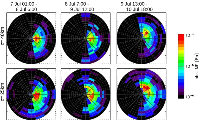
Figures 3 and 4 show momentum flux spectra for the three periods and altitude levels of 25 km and 40 km height ob-tained by Fourier Transform from winds (Fig. 3) and temper-atures (Fig. 4). Spectra are calculated in terms of horizontal wavenumbersk,land ground based frequencyω. From these the ground based phase speed (ch,x, ch,y) = (ω/ k, ω/ l) and propagation directionφ; l/ k= tan(φ)are calculated and the momentum flux values are binned accordingly.
The spectra are influenced by variations in the source as well as the filtering by the background winds. This is de-scribed in detail by Kim and Chun (2010) and here only salient patterns in the spectra are discussed. The effects of the background winds are similar in all three periods. Due to the background easterlies in the subtropical jet, part of the waves reaches a critical level around the tropopause. Down-stream (westward) propagating waves with low phase speeds are removed from the spectrum. Some waves with south-west or north-west propagation direction and some with phase speeds larger than 40 ms−1remain, but are weaker than the upstream (eastward) propagating waves. The effect intensi-fies at 40 km altitude where only waves in the right-hand side of the plots (i.e. preferentially upstream propagating GWs) remain.
Fig. 2. Comparison of different methods to infer the momentum flux. Shown are results for the three periods and both zonal and meridional
momentum. Long-dashed lines indicate negative, dashed lines positive and solid lines net momentum fluxes. Please note that the S3D results are reliable only above 25 km.
highlighted by a purple box in Fig. 4, lower left spectrum. If the waves propagating upward from the source meet the background winds from about−10 to−40 m s−1, i.e. do not meet zero wind, critical-level filtering occurs only for wave components between these two critical lines resulting in the pig-tail shape spectrum. The variation among the periods is mainly due to differences in the wave excitation. In the first period the typhoon propagates north-westward, in the second
period northward and in the third period north-eastward. In the second period the typhoon emits GWs with a slight ward preference, in the third period there is a strong north-east preference in the wave excitation.
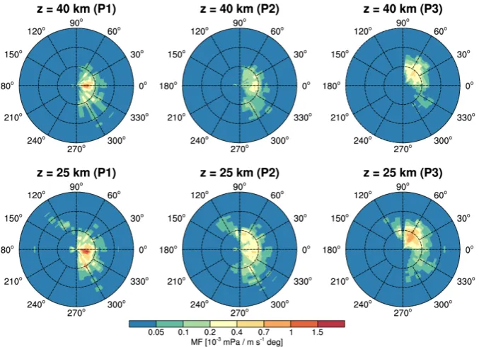
The corresponding spectra from the S3D analysis are shown in Figs. 5 and 6. The momentum flux is the abso-lute valueFp=
q
F2
C. I. Lehmann et al.: Consistency of different spectral methods for GW analysis 1643
Fig. 3. Momentum flux spectra calculated from model winds for 25 km and 40 km altitude. Spectra are calculated in terms ofk,land ground
based frequencyωgb and binned according to ground based phase speed and propagation direction. The radial coordinate is phase speed, origin is 0 ms−1, circles give phase speeds of 20 ms−1, 40 ms−1and 60 ms−1. Momentum flux is determined from co-spectra of vertical and horizontal winds. Note the quasi-logarithmic color scale.
are calculated from the wave vector and background winds (cf. Sect. 2.2).1 The S3D method was applied to the data at the full hour only (FT was applied to 10 min sampling). Therefore, there are too few points to obtain as fine a spec-tral grid as used for the FT results. This also results in dif-ferent absolute values per spectral bin and we therefore will focus on the relative structures. It should be further noted that Figs. 5 and 6 are plotted using a logarithmic color scale and resolve smaller momentum flux values than the color scales used in Figs. 3 and 4.
In comparing the spectra, all salient structures described above are well reproduced by the S3D method. Both the wind filtering between the two levels as well as the change of wave excitation between the different periods can be observed. The predominant phase speeds are well captured. Also the little “pig tail” is reproduced.
1For the wind spectra the zonal momentum flux (respectively the meridional momentum flux) is directly calculated from the zonal and vertical wind amplitudesuˆ andwˆ and the phase differenceψ:
Fp,x=uˆwˆ cosψ. In this way we obtain for each wave solution also a direction of the momentum fluxφF;Fp,y/Fp,x= tan(φF). How-ever, as we need also the phase speed, we bin according to the prop-agation direction determined from the wave vectorφ;l/ k= tan(φ).
5 Spatio-temporal variations
Strong convection is a localized source. GWs are expected to be radiated away from this source, i.e. eastward propa-gating waves are observed predominately east of the convec-tion and westward propagating waves are observed predomi-nately west of the convection (e.g. Piani et al., 2000; Alexan-der et al., 2004). However, a typhoon is a very complex sys-tem encompassing strong convection in the eye-wall as well as in the spiral bands. Therefore, the relative location of the observed GWs with respect to the storm center can give fur-ther insight in the details of the generation mechanism.
Also of interest is the temporal development. From the spectra it can be seen that the typhoon changes its GW radi-ation characteristic between the three periods with a distinct preference of generating north-eastward propagating waves (in the same direction as the propagation direction of the ty-phoon) during period 3. Is it also possible to achieve a finer temporal resolution?
Fig. 4. As Fig. 3 but for model temperatures. Polarization relations are employed to calculate the momentum flux from the temperature
amplitudes.
z= 25km
z= 40km
9 Jul 13:00 10 Jul 18:00 8 Jul 7:00
9 Jul 12:00 7 Jul 01:00
8 Jul 6:00
Fig. 5. Momentum flux spectra from the S3D analysis method applied to model winds. The radial coordinate is phase speed, origin is 0 ms−1,
circles give phase speeds of 20 ms−1, 40 ms−1and 60 ms−1. The ground-based phase speed is determined from the vertical wavelength and background winds. Color scale is logarithmic.
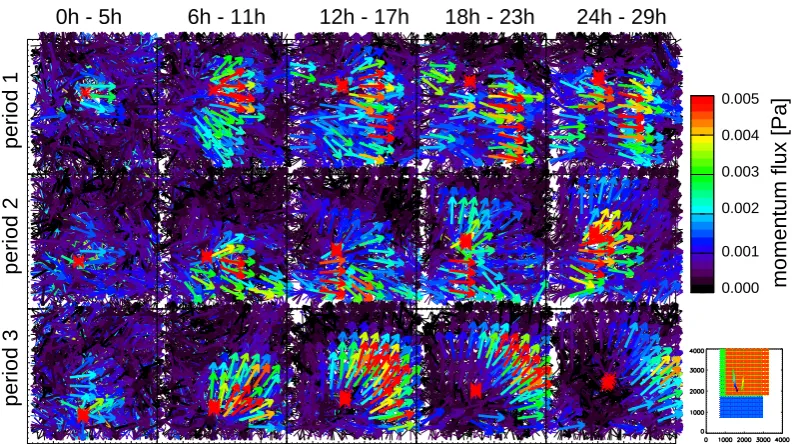
direction of the momentum flux, the color gives the abso-lute value. The thick arrows show the sum of the two com-ponents and the average over the six hours, that is the av-erage total momentum flux for every spatial analysis vol-ume of 360 km×360 km×10 km. The red asterisks mark the position of the typhoon center. The small panel below the color bar indicates the center positions of the analysis volumes (crosses) and the typhoon track with respect to the
total model domain for the three periods. In this panel color indicates time.
C. I. Lehmann et al.: Consistency of different spectral methods for GW analysis 1645
z= 25km
z= 40km
9 Jul 13:00 10 Jul 18:00 8 Jul 7:00
9 Jul 12:00 7 Jul 01:00
8 Jul 6:00
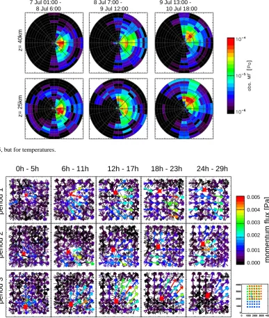
Fig. 6. As Fig. 5, but for temperatures.
0h - 5h
6h - 11h
12h - 17h
18h - 23h
24h - 29h
period 3
period 2
period 1
momentum flux [Pa]
0.005
0.004
0.003
0.002
0.001
0.000
Fig. 7. Spatio-temporal evolution of the the momentum flux over the typhoon at 25 km altitude for 360 km×360 km×10 km analysis
volume. Thin arrows indicate single events and components, thick arrows the average total momentum flux. Each panel shows a six hourly interval, time proceeds from left to right and top to bottom. Please note that the position of a momentum flux value corresponds to the center of an arrow (not the base!).
To confirm the interpretation, Fig. 11 shows the accumulated precipitation of the last hour before the mid of each period. The white frame indicates the analysis region and the white asterisk the typhoon center.
Physical interpretation of results
Comparing the thin arrows which show the individual fits, i.e. single wave events, with the thick arrows which give the sum of both spectral components and the averages over 6 h,
i.e. the average total momentum flux in Figs. 7 and 8, re-gional differences are found. In regions with low momentum flux, the direction is often almost arbitrary resulting in arrows pointing in all directions. For the regions of large momentum flux also the single events are more coherent though some variations exist.
Even better spatial resolution can be reached, if the size of the analysis volumes is reduced to 189 km×
0h - 5h
6h - 11h
12h - 17h
18h - 23h
24h - 29h
period 3
period 2
period 1
momentum flux [Pa]
0.005
0.004
0.003
0.002
0.001
0.000
Fig. 8. As for Fig. 7 but for 40 km altitude.
0h - 5h
6h - 11h
12h - 17h
18h - 23h
24h - 29h
period 3
period 2
period 1
momentum flux [Pa]
0.005
0.004
0.003
0.002
0.001
0.000
Fig. 9. As for Fig. 7 but for 189 km×189 km×10 km analysis volume. Please note that the position of a momentum flux value corresponds
to the center of an arrow (not the base!).
The magnitude of the momentum flux values as well as the salient features are the same as in Figs. 7 and 8, but finer detail is resolved and the patterns can be interpreted more easily.
First the distributions at 25 km altitude (Figs. 7 and 9) are considered. In the beginning of period 1 (first row, sec-ond column), the largest momentum fluxes are arc oriented around the typhoon center and with the highest values close to the center. It should, however, be noted that the direction of the arrows is not away from the storm center but stronger
W–E oriented and extends rather far to the south. This is consistent with a large region of precipitation observed in Fig. 11, left panel, which acts also as a wave source and is located in the south of the typhoon center.
C. I. Lehmann et al.: Consistency of different spectral methods for GW analysis 1647
0h - 5h
6h - 11h
12h - 17h
18h - 23h
24h - 29h
period 3
period 2
period 1
momentum flux [Pa]
0.005
0.004
0.003
0.002
0.001
0.000
Fig. 10. As for Fig. 8 but for 189 km×189 km×10 km analysis volume.
07-Jul-2006 15:00 UTC 08-Jul-2006 21:00 UTC 10-Jul-2006 03:00 UTC
Fig. 11. Accumulated precipitation of the last hour before the center time of each simulation period. The white frame indicates the analysis
region and the white asterisk the typhoon center.
precipitation in the north seems to be connected to a large area of moderate momentum flux (about 0.5 mPa).
In period 3 these north and north-eastward propagating waves become the dominant features. The waves are clearly connected to the typhoon center. Towards the end of period 3, the intensity of the storm decreases (two rightmost panels, lower row). In accordance, the momentum flux considerably weakens. Again this can also be seen in Fig. 11, where the accumulated precipitation decreases.
At 40 km altitude (Figs. 8 and 10) the waves have, in gen-eral, propagated away from the storm center and upstream. This effect is best noticeable in the third period. In the very last panel the maximum of gravity wave momentum flux seems to extend outside the analysis region, which was cho-sen to match the region of the FT. Relative maxima in mo-mentum flux occur somewhat later which is compatible to a non-zero group velocity of the GWs.
In summary, the S3D method reveals strong spatial vari-ations which are related to the position of the waves with respect to the storm center. The spatial variations are plausi-ble in terms of waves radiating away from a common source. Such spatial inhomogeneities are at odds with the theoretical basis of a FT postulating a homogeneous wave field.2
Compared to a mere variance analysis the S3D method could also provide such parameters as phase speed and group velocity as well as a full wave characterization allowing ray-tracing experiments.
6 Summary and discussion
Our case study demonstrates that inside a range of 10–20 % or better, the two different approaches, that is (1) a FT spec-tral decomposition of an assumed-to-be homogeneous region and (2) spatially varying few-wave superpositions are consis-tent. This is very comforting, since a single true approach that can serve as a kind of “silver bullet” does not exist, and compromises have always to be made. Basic consistency is even reached for a homogeneous spectrum as shown in Appendix A. Both approaches have their strengths (+) and weaknesses (−).
Fourier transform
o is a multi-spectral approach assuming spatial homogeneity
+ has a long tradition and well founded theoretical background
+ describes the variance completely (Parseval theorem) + provides well resolved spectra for
o the parts of the wave spectrum which are small compared to the analysis region or period
o fine and regular sampling
− is prone to leakage if the wavelength is of the same order of size as the analysis region
− maps spatial variation into spectral features Few-wave decomposition
+ assumes spatial homogeneity over a small volume only + has a simple mathematical background
+ can describe a superposition of a few waves and charac-terize them completely
+ provides solutions for any wavelengths, even those which are larger (at least in one or two dimensions) than the analysis volume
+ can provide spectra by superposition of the single vol-ume solutions
− may map superpositions of many waves or waves of similar frequency into spatial variations (cf. beat fre-quency effects may occur)
The essential advantage of the few-wave decomposition (S3D) for evaluation of measurements is that it can be per-formed with good results on relatively small volumes. Cur-rently, there are a few instruments which can provide 3-D data sets: nadir viewing satellites, though with very limited
vertical resolution, and novel radar systems. In future, limb imaging satellite instruments, if funded, also will provide 3-D data. In all these cases, the measurement volume is limited. Though a single measurement may not fully characterize the spectrum, in a statistical sense all important quantities such as characteristic phase speeds, preferential propagation di-rections and the relative contribution of positive and negative zonal and meridional fluxes can be achieved.
The S3D method may also be an interesting tool for an-alyzing model data. Global high-resolution model data are commonly only saved at time-steps much too sparse for a space-time analysis. While momentum flux and its direction can be directly calculated from the wind fields by spatial av-eraging, the chosen spatial region influences the result, su-perpositions of waves are not decomposed and spectral in-formation is missing. Few-wave decomposition may be an alternative, here.
In particular, the full 3-D wave vector together with back-ground winds allows S3D results to be used as launch param-eters for ray-tracing and thus opens a large potential for im-proved interpretation of measurements and model data alike.
Appendix A
Application of the S3D method to theoretical spectra
The method is inspired by the study of a potential new in-frared limb imager and is therefore applied to a stratospheric GW distribution above a complex GW source. It is suggested that it can be applied also to, e.g. model data for which space-time Fourier analysis is not possible, for instance high-resolution ECMWF data which are provided only at 6 h sam-pling. In such cases of complex sources it will reveal both spectral and spatial properties. However, introducing a new analysis method, we should also outline its limitations. We therefore perform a stringent test for an unfavorable condi-tion for S3D method and construct a test case in terms of a single source which generates a wide spectrum of GWs, such as e.g. a single latent heat release pulse. These GWs, having different wave vectors, phase speeds and group velocities, would reach the stratosphere at different locations and times. Unfortunately, we have no such test-case available. However, we can perform another stringent test and construct an arti-ficial spatial distribution obeying universal scaling laws. We first prescribe amplitudesA(k, l, m)according to
A(k, l, m)=A0
k
k∗
pl
l∗
p m
m∗
r
(A1)
with(k, l, m)the respective wavenumbers in(x, y, z)
C. I. Lehmann et al.: Consistency of different spectral methods for GW analysis 1649
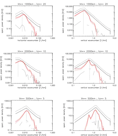
Fig. A1. Comparison of (red) S3D and (black) 1-D Fourier transform spectra for (left column) horizontal and (right column) vertical
coordi-nates. The solid lines give the average spectrum, dashed lines for the FT show the standard deviation of all 1-D FT spectra in one data set. We have repeated the whole experiment for 100 independent random phase configurations: the according standard deviation is denoted for the S3D method by dashed lines.
for smallmandr=−3 for largem. The spatial distribution is then constructed via FFT by superposing all these waves with random phases. By definition, in this test case the whole spatial domain is completely filled by homogeneous waves. Since the distribution is constructed separable, also 1-D FFT in the respective spatial dimension can be applied and the average of all 1-D profiles be compared to the S3D method.
Examples shown are for a total volume of 121×
121×105 points with 25 km horizontal and 0.5 km verti-cal sampling analyzed by S3D cubes of 11 points in the
FFT
S3D
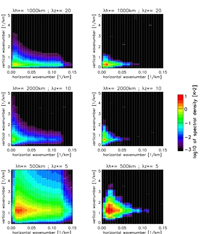
Fig. A2. Comparison of (left panels) Fourier transform and (right panels) S3D spectral intensity versus horizontal (k2+l2) and vertical
wavenumber.
We achieve the following results: By S3D we find broad spectral distributions peaking at about the position of (k∗, l∗, m∗). The further the spectral distance of the wave vector from the “characteristic” wave vector is the larger the underestimate of the S3D. In particular, for spectral compo-nents where the intensity is less than one order of magni-tude than the peak value, S3D heavily underestimates the intensities. In addition, S3D also overestimates some verti-cal wavelengths which are an integer fraction or multiple of
C. I. Lehmann et al.: Consistency of different spectral methods for GW analysis 1651
average over these regions. The separation of spectral com-ponents by GWs taking different paths when propagating up-ward, may add to this effect. This is a situation which is typ-ical for stratospheric measurements, e.g. made by a future infrared limb imager. In all cases where a sufficiently large ensemble of not-too homogeneous forcing is analyzed, S3D will perform well; homogeneous spectra are moderately well characterized. If homogeneous spectra are expected, Fourier transform is the better choice, provided that the data allow this method. However, if a region is probed by a multitude of independent small-volume measurements and FT therefore cannot be applied, S3D is still a way to estimate the salient spectral features.
Acknowledgements. This work was funded by ESA under the grant “Observation of Gravity Waves from Space”, contract number: 22561/09/NL/AF.
The service charges for this open access publication have been covered by a Research Centre of the Helmholtz Association.
Edited by: S. Malinowski
References
Alexander, M. J. and Ortland, D. A.: Equatorial waves in High Res-olution Dynamics Limb Sounder (HIRDLS) data, J. Geophys. Res., 115, D24111, doi:10.1029/2010JD014782, 2010.
Alexander, M. J., May, P. T., and Beres, J. H.: Gravity waves generated by convection in the Darwin area during the Dar-win Area Wave Experiment, J. Geophys. Res., 109, D20S04, doi:10.1029/2004JD004729, 2004.
Alexander, M. J., Geller, M., McLandress, C., Polavarapu, S., Preusse, P., Sassi, F., Sato, K., Eckermann, S., Ern, M., Hertzog, A., Kawatani, Y., Pulido, M., Shaw, T. A., Sigmond, M., Vin-cent, R., and Watanabe, S.: Recent developments in gravity-wave effects in climate models and the global distribution of gravity-wave momentum flux from observations and models, Q. J. Roy. Meteorol. Soc., 136, 1103–1124, 2010.
Butchart, N., Cionni, I., Eyring, V., Shepherd, T. G., Waugh, D. W., Akiyoshi, H., Austin, J., Bruehl, C., Chipperfield, M. P., Cordero, E., Dameris, M., Deckert, R., Dhomse, S., Frith, S. M., Gar-cia, R. R., Gettelman, A., Giorgetta, M. A., Kinnison, D. E., Li, F., Mancini, E., McLandress, C., Pawson, S., Pitari, G., Plum-mer, D. A., Rozanov, E., Sassi, F., Scinocca, J. F., Shibata, K., Steil, B., and Tian, W.: Chemistry-climate model simula-tions of twenty-first century stratospheric climate and circulation changes, J. Climate, 23, 5349–5374, 2010.
Dunkerton, T. J.: The role of gravity waves in the quasi-biennial oscillation, J. Geophys. Res., 102, 26053–26076, 1997. Ern, M. and Preusse, P.: Quantification of the contribution of
equa-torial Kelvin waves to the QBO wind reversal in the stratosphere, Geophys. Res. Lett., 36, L21801, doi:10.1029/2009GL040493, 2009.
Ern, M., Preusse, P., Alexander, M. J., and Warner, C. D.: Absolute values of gravity wave momentum flux de-rived from satellite data, J. Geophys. Res., 109, D20103, doi:10.1029/2004JD004752, 2004.
Fritts, D. C. and Alexander, M. J.: Gravity wave dynamics and effects in the middle atmosphere, Rev. Geophys., 41, 1003, doi:10.1029/2001RG000106, 2003.
Kerridge, B., Hoffmann, L., Preusse, P., Riese, M., Hoepfner, M., Glatthor, N., Friedl-Vallon, F., Kleinert, A., Orphal, J., Dudhia, A., Urban, J., Eriksson, P., Lossow, S., Murtagh, D., Murk, A., Whale, M., van Weele, M., McConnell, J., Kaminski, J., Lupu, A., Semeniuk, K., Siddans, R., Reburn, J., Waterfall, A., Latter, B., and Miles, G.: PREMIER – consolidation of requirements and synergistic retrieval algorithms, Final Report of ESA con-tract 4200022848/09/NL/CT, ESA Communication Production Office ESTEC, Noordwijk, The Netherlands, 2012.
Kim, S.-Y. and Chun, H.-Y.: Momentum flux of stratospheric grav-ity waves generated by typhoon Ewiniar (2006), Asia-Pacific J. Atmos. Sci., 46, 199–208, 2010.
Kim, S.-Y., Chun, H.-Y., and Wu, D. L.: A study on stratospheric gravity waves generated by typhoon Ewiniar: Numerical simula-tions and satellite observasimula-tions, J. Geophys. Res., 114, D22104, doi:10.1029/2009JD011971, 2009.
Kim, Y.-H., Chun, H.-Y., Preusse, P., Ern, M., and Kim, S.-Y.: Gravity wave reflection and its influence on the consistency of temperature- and wind-based momentum fluxes simulated above Typhoon Ewiniar, Atmos. Chem. Phys. Discuss., 12, 6263–6282, doi:10.5194/acpd-12-6263-2012, 2012.
McLandress, C.: On the importance of gravity waves in the middle atmosphere and their parameterization in general cir-culation models, J. Atmos. Sol.-Terr. Phys., 60, 1357–1383, doi:10.1016/S1364-6826(98)00061-3, 1998.
McLandress, C. and Shepherd, T. G.: Simulated anthropogenic changes in the Brewer-Dobson circulation, including its exten-sion to high latitudes, J. Climate, 22, 1516–1540, 2009. Piani, C., Durran, D., Alexander, M. J., and Holton, J. R.: A
numer-ical study of three-dimensional gravity waves triggered by deep convection and their role in the dynamics of the QBO, J. Atmos. Sci., 57, 3689–3702, 2000.
Preusse, P., Ern, M., Eckermann, S. D., Warner, C. D., Picard, R. H., Knieling, P., Krebsbach, M., Russel III, J. M., Mlynczak, M. G., Mertens, C. J., and Riese, M.: Tropopause to mesopause gravity waves in August: measurement and modeling, J. Atmos. Sol.-Terr. Phys., 68, 1730–1751, 2006.
Preusse, P., Schroeder, S., Hoffmann, L., Ern, M., Friedl-Vallon, F., Ungermann, J., Oelhaf, H., Fischer, H., and Riese, M.: New perspectives on gravity wave remote sensing by space-borne infrared limb imaging, Atmos. Meas. Tech., 2, 299–311, doi:10.5194/amt-2-299-2009, 2009.
Skamarock, W. C., Klemp, J. B., Dudhia, J., Gill, D. O., Barker, D. M., Duda, M. G., Huang, X.-Y., Wang, W., and Powers, J. G.: A description of the Advanced Research WRF Version 2, NCAR Tech Note, National Center for Atmospheric Research, Boulder, CO, USA, 488–494, 2005.