www.nonlin-processes-geophys.net/19/227/2012/ doi:10.5194/npg-19-227-2012
© Author(s) 2012. CC Attribution 3.0 License.
Nonlinear Processes
in Geophysics
Multifractal detrended fluctuation analysis in examining scaling
properties of the spatial patterns of soil water storage
A. Biswas1,3, T. B. Zeleke2, and B. C. Si3
1CSIRO Land and Water, Canberra, Acton, ACT, 2601, Australia
2Paragon Soil and Environmental Consulting Inc., Edmonton, Alberta, T5L2N9, Canada
3Department of Soil Science, University of Saskatchewan, Saskatoon, Saskatchewan, S7N5A8, Canada
Correspondence to: A. Biswas ([email protected])
Received: 3 January 2012 – Revised: 24 February 2012 – Accepted: 10 March 2012 – Published: 27 March 2012
Abstract. Knowledge about the scaling properties of soil water storage is crucial in transferring locally measured fluc-tuations to larger scales and vice-versa. Studies based on remotely sensed data have shown that the variability in sur-face soil water has clear scaling properties (i.e., statistically self similar) over a wider range of spatial scales. However, the scaling property of soil water storage to a certain depth at a field scale is not well understood. The major challenges in scaling analysis for soil water are the presence of localized trends and nonstationarities in the spatial series. The objec-tive of this study was to characterize scaling properties of soil water storage variability through multifractal detrended fluctuation analysis (MFDFA). A field experiment was con-ducted in a sub-humid climate at Alvena, Saskatchewan, Canada. A north-south transect of 624-m long was estab-lished on a rolling landscape. Soil water storage was moni-tored weekly between 2002 and 2005 at 104 locations along the transect. The spatial scaling property of the surface 0 to 40 cm depth was characterized using the MFDFA technique for six of the soil water content series (all gravimetrically determined) representing soil water storage after snowmelt, rainfall, and evapotranspiration. For the studied transect, scaling properties of soil water storage are different between drier periods and wet periods. It also appears that local con-trols such as site topography and texture (that dominantly control the pattern during wet states) results in multiscaling property. The nonlocal controls such as evapotranspiration results in the reduction of the degree of multiscaling and im-provement in the simple scaling. Therefore, the scaling prop-erty of soil water storage is a function of both soil moisture status and the spatial extent considered.
1 Introduction
The spatial and temporal pattern of soil water storage is an important input variable in assessing land-atmosphere in-teractions, infiltration, recharge, and performance of engi-neered covers. Water storage is also a key input in monitor-ing the soil water balance and validation of several models (Rodriguez-Iturbe et al., 1999). The variability in soil water storage is shown to be strongly related to topographic, ge-ologic, soil, and vegetation parameters (Braud et al., 1995; Moore et al., 1988). These physical factors and environmen-tal processes (rainfall, evapotranspiration, runoff, and snow melt) do not operate independently, but as an ensemble of processes with a complex and nested effects. This, in turn, re-sults in a pattern of soil water storage that varies as a function of spatial scale. Several studies have reported a scale depen-dent pattern and variability of soil water storage (Kachanoski and de Jong, 1988; Gomez-Plaza et al., 2000; Kim and Bar-ros, 2002; Biswas and Si, 2011a).
228 A. Biswas et al.: Multifractal detrended fluctuation analysis
utilized in specific land management practices and precision agriculture provided that the observed scaling law holds at a field scale and to a deeper soil depth. This will also open a window of opportunity during aggregation of point mea-surements and disaggregation of remotely sensed data (Lin, 2003). However, a priori assumption of similarity in scaling laws between the fluctuations in the remotely sensed large scale and small field scale soil water storage data could be er-roneous owing to the increased importance of localized fac-tors as the resolution increases and need separate treatment.
Spatial variability includes spatial trends (non-stationary) and fluctuations (stationary). Several studies have indicated that non stationarities introduce superficial scaling features (Bhattacharaya et al., 1983; Koscielny-Bunde et al., 2006). Such scaling features are not intrinsic to the variables under study because they are artifacts of erroneously treating non-stationary fields as non-stationary. Nor do they reflect the actual in situ fluctuation that is the result of numerous co-existing and interacting factors and processes, and hence, scale trans-formations based on such relationships could be erroneous. To remove the undue influence of the larger scale trends on the scaling properties at a scale of interest, there is a need to identify the intrinsic scaling property of the fluctuation in soil water storage at a field scale that results from interaction of all the underlying processes. Also there is a need to evaluate the presence as well as extent of spatial scales with a partic-ular scaling property. Such analysis is useful in defining the spatial extent over which simple scaling up of point observa-tions is possible as well as predicting soil water based on the observed scaling laws.
Soil water distribution within heterogeneous fields is often complex owing to the numerous physical factors and pro-cesses controlling its spatial and temporal variability. The large scale processes results in long-range correlations, with an autocorrelation (two-point correlation) function decaying slowly with increase in separation distance. If the two-point correlation function decays as a power-law, we have a scal-ing phenomenon. The power spectrumP (f ), which is the Fourier transformation of the correlation function, will also be a power-law function: P (f )=f−c, wheref is the fre-quency and c is the scaling exponent. However, the two-point correlation function may not be the best way to char-acterize the long-range correlation, because it does not take into account of the structures in between two points, and it does not measure correlation between two units larger than a point. As the long-range correlation is very common in nature, engineering, and medicine, many methods have been developed to analyze the scaling property in the long-range correlation. Proven methods that remove nonstationarities from the data series include the Hurst rescaled-range anal-ysis (Hurst, 1951), the wavelet transform modulus maxima (WTMM; Arneodo et al., 2002; Zeleke and Si, 2007), and the detrended fluctuation analysis (DFA) (Peng et al., 1992, 1994). The Hurst re-scaled range analysis is based only on the first moment of the series and hence does not provide the
detailed characterization of the spatial statistics, nor does it remove nonstationarities (Liebovitch et al., 2002; Koscielny-Bunde et al., 2006). Similar to the wavelet transform (Mallat, 1999), the WTMM is easily applied to binary observations (i.e.,n= 2k, wheren= number of observations andk= 1, 2, 3, 4...) for its computational simplicity and to minimize “edge effects” (Mallat and Hwang, 1992; O´swie¸cimka et al., 2005). The DFA, on the other hand, is more computationally simple, straight forward and flexible technique and does not depend on any specific number of observations (e.g., binary obser-vations) given it covers the scales of interest (Kantelhardt et al., 2002; O´swie¸cimka et al., 2005; Koscielny-Bunde et al., 2006). Integration of the data series reduces outliers that usually exist in spatial data whereas the detrending proce-dure reduces the effect of nonstationarities. The DFA tech-nique, originally developed for monofractal variables, has been extended to accommodate analysis of scaling hetero-geneity through multifractal detrended fluctuation analysis (MFDFA; Kantelhardt et al., 2002). This development was achieved through modification of the traditional Hurst func-tion,Hinto a generalized function,h(q)so that moments of different orderscan be evaluated. A detailed comparison be-tween WTMM and MFDFA can be found in Kantelhardt et al. (2002).
2 Theory
2.1 Scaling analysis based on the detrended fluctuation series
The DFA for a one dimensional data series can be described as follows. LetXj be a data series of lengthN with a
com-pact support (j=1,2,···, N ). The integrated series or the profile at locationi,Y (i), is determined by taking the sum of deviations from the mean value (Kantelhardt et al., 2002; Telesca et al., 2004) i.e.,
Y (i)=
i
X
k=1
(Xk− hXi), i=1,2,···,N (1)
wherehXiis the mean value of the series forNobservations. The integrated series Y (i) is then divided into Ns
non-overlapping segments of equal sizes. Since the lengthN of the series may not be a multiple ofs, an unequal and short part (< s) of the profile may left at the end. In order not to disregard this part of the series, the same procedure is re-peated starting from the other end. Thus, 2Ns segments are
obtained altogether. Then the local trend for each of the 2Ns
segments is calculated by a least squares fit of a polynomial function.
The mean squared difference between the series [Y (i)] and the ordinate of the fitted polynomial [yv(i)] is calculated as
F (s,v)=1
s
s
X
i=1
{Y ((v−1)s+i)−yv(i)}2 (2)
Note that the indicesiandvcorrespond to the original data points and the segments of sizes, respectively. TheF (s,v) is used to calculate the fluctuation functions as follows. The standard fluctuation function,F2(s)is calculated as a square
root of the average ofF (s,v)over all the segments of sizes, i.e.,
F2(s)=
1 2Ns
v u u t
2Ns X
v=1
F (s,v) (3)
The standard fluctuation function is based on the variance (second order moment) of the fluctuation of observed values relative to fitted polynomial trends. The fluctuation function can be extended to include higher order moments (sayq val-ues) to analyze the scaling property of different ranges of fluctuations, and also the detrending polynomial,yvcan take
any ordern(linear, quadratic, cubic, etc.). The generalized fluctuation function,Fq(s)is thus defined as
Fq(s)=
(
1 2Ns
2Ns X
v=1
[F (s,v)]q/2
)1/q
(4)
where the variableq can take any real value except zero. In the case whereq is zero, the fluctuation function cannot be determined directly from Eq. (4) because of the diverging
exponent. Thus,F0(s)is approximated by taking the
loga-rithmic average as,
F0(s)=exp (
1 4Ns
2Ns X
v=1
ln[F (s,v)]
)
(5)
Repeating the above procedure for several length scales, a re-lationship can be developed between the fluctuation function and the segment length. Typically,Fq(s)will increase with
increase in scales. If the seriesXi has a long range power
law correlation,Fq(s)increases with increase insas a power
law
Fq(s)∝sh(q) (6)
whereh(q)is the generalized Hurst scaling function (Telesca et al., 2004). Forq= 2 we have the standard DFA analysis. In this case, the scaling exponenth(2) provides information about the average fluctuation of the series. The series can be categorized into one of the following three types depend-ing on theh(2) value. These are: (i) 0< h(2)<0.5 for an anti-persistent type long range correlated process where large values (compared to the average) are more likely followed by small values and vice versa, (ii)h(2) = 0.5 for an entirely random uncorrelated distribution, and (iii) 0.5< h(2)<1 for a persistent and long range correlated process where large values are more likely to be followed by large values and vice versa.
2.2 Scaling heterogeneity (multifractality) of the detrended fluctuation series
The link between the generalized fluctuation function and the standard box counting formalism of multifractal analysis is also a straight forward one (Kantelhardt et al., 2002). For a normalized seriesXk, the mass distribution probability in the
v-th segment of sizesunit,Ps(v), can be calculated as
Ps(v)= vs
X
k=(v−1)s+1
Xk=Y (vs)−Y[(v−1)s] (7)
The mass scaling function,τ(q)is then defined via the parti-tion funcparti-tionµ(q,s)as,
µ(q,s)=
N/s
X
v=1
|Ps(s)|q∝sτ (q) (8)
The mass scaling function is related to the generalized Hurst scaling function,h(q)as (Kantelhardt et al., 2002)
τ (q)=qh(q)−1 . (9)
230 A. Biswas et al.: Multifractal detrended fluctuation analysis
therefore needs more in-depth and rigorous testing of the pro-posed relationship,
τ (q)=qh(q)−qH0−1. (10)
whereH0 is the non-conservation parameter in the univer-sal multifractal formalism. Therefore, in this manuscript we have used the well established relationship betweenτ (q)and h(q)proposed by Kantelhardt et al. (2002).
The singularity spectrum of a multifractal measure,f (α), is related toτ (q)via a Legendre transform as (Feder, 1988)
f (α)=qα−τ (q) (11)
where,αis a singularity strength or H¨older exponent and ob-tained numerically as the first derivative of theτ (q)function with respect toq. Hencef (α)denotes the dimension of the subset of the series that is characterized byαherefore,f (α) can be used during the multifractal analysis for convenience and ease of interpretation once the series is normalized, inte-grated, and detrended using the appropriate detrending poly-nomial.
Schertzer and Lovejoy (1987) derived a universal multi-fractal (UM) model based in certain reasonable assumptions about the mechanism generating multifractals. The critical assumption was that the underlying generator is a random variable with an exponentiated extremal L´evy distribution (Zeleke and Si, 2006). The UM model can describe theτ(q) function under the assumption of conservation of mean value of the variable.
τ (q)= C1
α0−1(qα 0
−q) α06=1
C1.log(q) α0=1 (12)
where,α0(commonly known as L´evy index) indicates the de-gree of multifractality based on the deviation ofτ(q) function from a monofractal type of scaling (UM model) (Seuront et al., 1999) andC1 indicates the co-dimension between obser-vation space and fractal dimension.
Nonstationarity is a common aspect of complex variability and is often be associated with different trends in the data se-ries or patches with different local statistical properties (Kan-telhardt et al., 2001). The DFA approach described above reduces the effect of such nonstationarities on scaling prop-erty of a variable. The reason for detrending analysis is to remove the undue influence of larger (than the scale of inter-est) scale on the statistics of soil water at the scale. At small scale, we remove trends of small scale; at large scale, we re-move only large scale trend and small scale trend remains, because the small scale trends do not affect the scaling prop-erties at a large scale. Therefore, we do not lose any criti-cal information in soil water content. This is evident from the following three key aspects of the method. Firstly, the original series (i.e., as determined by all hydrological pro-cesses) is integrated into a continuous profile by summing up the deviations from the mean value (see Eqs. 1 and 2). In other words, the integrated profile of the series is the result of
all the processes determining the spatial pattern of the vari-able. Secondly, the integrated profile was divided into ments and regression lines were fitted to each of these seg-ments (window). When the fitted trends are removed, what remains is a fluctuation function, which is the difference be-tween the integrated series and its best fit regression line at a given window size. This function contains all the local as well as global feature of the data series which is free from nonstationarities. Thirdly, the size of the segment (the win-dow) was continuously varied later on; i.e., during the scaling analysis. At this step, it is important to note that the scaling property is determined by relating the fluctuation function to several window sizes (Eq. 6). These points clearly show that the DFA procedure does not exclude any process that deter-mine the hydrology of the system; rather transform resulting data series into a fluctuation function where the effect of non-stationarities is significantly reduced. Thus, in essence, the main advantage of the DFA method is that it allows detection of scaling property of a physical variable that is embedded in a noisy data or containing monotonous polynomial trends that can mask true fluctuations of the series.
3 Material and methods
The study site is located in a sub-humid climate at Alvena, Saskatchewan, Canada. The geographical location of Alvena is 49◦440N latitude and 107◦350W longitude. The site has rolling topography (locally referred to as a hummocky ter-rain) with a dominant soil type of an Aridic Ustoll (US Soil Taxonomy). The surface texture is loam to clay loam. Long term mean annual air temperature is 2.2◦C and precipitation is 350 mm. The potential evapotranspiration is 624 mm yr−1,
Western and Bl¨oschl (1999). For instance, taking the mean value of four consecutive discrete samples that are initially spaced 3 m apart is equivalent to increasing the scale from 3 m to 12 m. In this transform both the spacing and sup-port are upscaled. In other words, we are increasing both the spacing and support (i.e., making a practical assumption that the mean value is representative of the length within the spacing).
Water content was measured following the standard gravi-metric technique (Gardner, 1986). The core samples were collected from each measurement locations using a 5 cm (in-ternal) diameter sampler that was vertically mounted on a truck with a hydraulic system. The undisturbed core samples were sliced into 10 cm increments and placed in a plastic bag for oven drying. The mass based water content is determined as mass difference between the wet and oven-dry samples di-vided by the sampling volume. The bulk density of the sam-ple is determined as the oven dry mass of the soil samsam-ple di-vided by the sampling volume. The volumetric equivalent of the gravimetric water content of the samples was determined by multiplying the mass based water content with bulk den-sity. Mean values of four core samples, taken at 10 cm verti-cal intervals, was used to obtain a data point representing the surface 0 to 40 cm depth. Soil water storage in the root zone is critical to plant productivity. The top 60 cm have majority of roots. However, soil water content at depth determined us-ing gravimetric methods may not be accurate because of the potential compaction when a punch truck is used to extract soil cores in the clay soil. Our experience in this field sug-gested that 40 cm depth is free of observable compaction and therefore, we chose 40 cm.
Particle size distribution of the soil samples were deter-mined from the first measurement sets using the hydrome-ter method (Gee and Bauder, 1986). Organic carbon content was determined using LECO-12 carbon determinator (LECO Corporation, St. Joseph, MI). Relative elevation along the transect was determined using a Laser Theodolite Total Sta-tion (Sokkisha Electronic Total StaSta-tion, Set 5, Sokkisha, Tokyo, Japan). Both the DFA and MFDFA analysis were per-formed using programs written in Mathcad Professional (ver-sion 12, Mathsoft Inc., Cambridge, MA, 2002) and Statistical Analyses Software- SAS Version 8 (SAS Institute Inc., Cary, NC).
4 Results and discussions
4.1 Water storage series and order of detrending polynomials
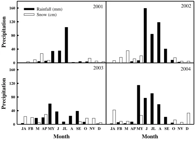
Figure 1 shows the spatial distribution of soil water storage at six occasions, two soil properties (clay and organic car-bon) and one topographic variable (relative elevation). The monthly mean precipitation values for the years 2002 to 2004 are shown in Fig. 2. The total precipitation received in the
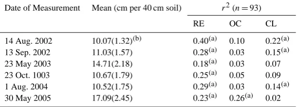
calendar years of 2002 and 2004 was generally higher than the long term average precipitation of the area and these years are regarded as wet years. However, high soil water storage was observed only in May 2003 and 2005. The ob-served high soil water in the two series compared to others appears to be the result of relatively high snow fall in the months preceding the measurements and gradual melting of snow where downward infiltration significantly exceeds run off. Water storage during all the occasions were negatively correlated (r2=0.18 to 0.40; significant atp=0.01) to rel-ative elevation (RE) as expected (Table 1). The relationship to clay content (CL) was significant (r2=0.22, 0.15, and 0.14; significant atp=0.01) only for measurements taken in August 2002, September 2003, and August 2004. The variance in May 2003 and 2005 were higher than the other four series and appear to be caused by non uniform snow re-distribution and runoff related spatial variations. Although there were some significant (p=0.01) positive relationships to CL, the distribution of water storage was dominantly con-trolled by RE. Consequently, there were systematic and lo-calized trends in the spatial distribution of water storage at all scales that follows the landscape pattern. Prior to scal-ing property analysis, nonstationarities due to such localized trends have to be removed (or minimized) through transfer-ring the series into its fluctuation function. To this end, iden-tifying the correct order of the detrending polynomial is the initial step.
232 A. Biswas et al.: Multifractal detrended fluctuation analysis
Figures
634
Water
Sto
rage
(cm
)
8 12 16 20
10 20 30
Distance
0 100 200 300 400 500
Elevati
on
-4 0
Std
.
valu
es
-2 0 2 4
August 14, 2002 September 14, 2002 May 23, 2003
October 23, 2003 August 1, 2004 May 30, 2005
Organic Carbon Clay
635
Fig. 1
636
Fig. 1. Spatial distributions of ( A and B) soil water storage (volumetric) at six occasions, (C) organic carbon and clay content, and (D)
relative elevation along the sampling transect at the study site . A standardized value of organic carbon and clay content is calculated (for presentation simplicity) by subtracting the average value from a particular value and dividing by the standard deviation of the whole spatial series.
Precipit
ation
0 40 80 120
160 Rainfall (mm) Snow (cm)
Month
JA FB M AP MY J JL A SE O NV D
Precipit
ation
0 40 80 120 160
Month
JA FB M AP MY J JL A SE O NV D
2004 2003
2001 2002
637
Fig. 2
638
Table 1. Mean and standard deviation of soil water storage at the Alvena site during six observation dates and relationships to relative elevations (RE), organic carbon (OC), and clay content (CL).
Date of Measurement Mean (cm per 40 cm soil) r2(n=93)
RE OC CL
14 Aug. 2002 10.07(1.32)(b) 0.40(a) 0.10 0.22(a)
13 Sep. 2002 11.03(1.57) 0.28(a) 0.03 0.15(a)
23 May 2003 14.71(2.18) 0.18(a) 0.03 0.07
23 Oct. 1003 10.67(1.79) 0.25(a) 0.05 0.09
1 Aug. 2004 10.52(1.75) 0.29(a) 0.03 0.14(a)
30 May 2005 17.09(2.45) 0.23(a) 0.26(a) 0.02
(a)Significant atp=0.01,(b)Standard deviation
about altering the intrinsic pattern of the series if the order of the detrending polynomial is too high (Kantelhardt et al., 2001). Bunde et al. (2002) reported that results are reliable only for certain orders, above which DFA yield the same type of behavior. Since the first order polynomial successfully re-moved majority of existing trends in our water storage data, it is reasonable to assume that the majority of the trends were of linear orders. Consequently, further scaling analysis was carried out using the first order detrended data series. 4.2 Evaluation of the DFA for scaling property
The standard fluctuation function (DFA2) was evaluated for power law relationships between fluctuations and scale. The fluctuations for all water storage series showed an almost ex-act power law increase with observation scales (Fig. 3). The coefficients of determination for a linear fit of the double-log plots of the series were between 0.99 and 1.00 (n=21). Such power law relationships indicate the presence of scaling laws (Hu et al., 1997).
4.3 Multifractal analysis
The scaling analysis presented above is based only on the second order moment or the variance of the fluctuation func-tion (i.e.,q=2). But in most physical and biological data the scaling property of low and high values (relative to the aver-age) is often different. Such observations imply the need for multifractal analysis in which the scaling property is repre-sented by an array of scaling exponents rather than by a sin-gle one. To this end, the scaling analysis has been extended by including higher and lower order moments (qvalues), i.e., in multifractal analysis (Eqs. 8, 9, and 11).
Mass exponents,τ (q) were derived from the fluctuation functions for q values between −20 and 20 and plotted against theq values (Fig. 4). A linear reference line (similar to monofractal type of scaling) (Fig. 4) was created following the UM model of Schertzer and Lovejoy (1987) to compare and characterize the observed scaling properties (Eq. 12). A
Table 2. Sum or Squared difference of Residuals between theτ(q) of the data and the simulated monofractal type distribution using UM model for the soil water storage of six observation dates.
Water storage series SSR Differences in variance ) (p=0.01, df = 39
14 Aug. 2002 670.91 SS
14 Sep. 2002 578.36 SS
23 May 2003 1392.00 SS
23 Oct. 2003 587.26 SS
1 Aug. 2004 535.18 SS
30 May 2005 1094.00 SS
SSR = Sum or Squared difference of Residuals between theτ(q)of the data and the simulated monofractal type distribution using UM model, SS = a significant difference (p <0.01) using Chi-square (χ2)goodness of fit test between theτ(q) of the data and the simulated model data, df = degrees of freedom used forχ2statistics evaluation, and p= probability.
chi-square test for goodness of fit (atp=0.01) indicate that all the soil water storage series are multifractal in nature as the mass exponent curve is quite different from the simulated monofractal type of scaling (Zeleke and Si, 2006). The sum of squared difference of residuals (SSR) of mass exponents and simulated monofractal type of scaling are summarized in Table 2. The SSR value for the soil water storage data series of 23 May 2003 and 30 May 2005 is way larger than the rest of the measurements indicating higher degree of multifrac-tality compare to other measurements. The high precipita-tion during the year of 2002 and 2004 led to high soil water storage. The post snow melt period as controlled by the sev-eral local and non-local controlling factors (Grayson et al., 1997) affected the spatial distribution of soil water storage making it more heterogeneous in nature. With time, heavy demand of evapotranspiration by plant community reduces this heterogeneity and the degree of multifractality towards fall season.
234 A. Biswas et al.: Multifractal detrended fluctuation analysis
LN (Scale)
1.5 2.0 2.5 3.0
LN(F2)
0 2 4 6
8 Aug. 14, 2002
H=0.91, R2=0.99 Sept14, 2002
H=0.80, R2=0.99 May 23, 2003
H=0.98, R2=1.00 Oct. 23, 2003
H=0.95, R2=1.00 Aug. 01, 2004
H=0.99, R2=1.00 May 30, 2005
H=0.72, R2=1.00
639
Fig. 3
640
Fig. 3. Double – logarithmic plots of the standard fluctuation functions fitted to linear equation. In order to avoid overlapping of the plots
(and hence difficulty in comparisons) a constant values have been added to the fluctuation functions of each series. “Scale” refers to a period (cycles) in meters.
q
-20 -10 0 10 20
Tau
-30 -20 -10 0 10 20 30
Aug. 14, 2002 Sept. 14, 2002 May 23, 2003 Oct. 23, 2003 Aug. 1, 2004 May 30, 2005 Linear reference
641
Fig. 4
642
Fig. 4. The mass exponents of the six soil water storage series (q= −20 to 20 at 1.0 increments). The solid line is a linear reference created following the UM model of Schertzer and Lovejoy (1987) passing throughτ(q=0).
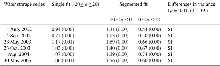
segmented (q= −20 to 0 andq=0 to 20) and summarized in Table 3. Statistical significance of the difference between the variances under these two cases was evaluated using the F statistics (Press et al., 1992). The difference between the variances under these two cases (single and segmented) was significant (p=0.01); implying that theτ (q)functions were significantly different from a linear function. A nonlinear τ (q)function means multiple scaling (Evertsz and Mandel-brot, 1992; Olsson and Niemczynowicz, 1996), which re-quires a hierarchy of scaling exponents (multiscaling) in or-der to accurately represent the scaling property. The degree of non-linearity ofτ(q)function can give idea about the
de-(q)
0.3 0.6 0.9 1.2 1.5 1.8
f(q)
0.0 0.3 0.6 0.9 1.2
Aug. 14, 2002 Sept. 14, 2002 May 23, 2003 Oct. 23, 2003 Aug. 1, 2004 May 30, 2005
643
Fig. 5
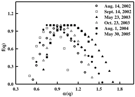
644 Fig. 5. The multifractal spectra of the water storage series (q=−20 to 20 at 1.0 increments).
gree of multifractality. The slope difference between seg-mented fractions of theτ(q)function of soil water storage are 1.03 and 0.95 respectively for 23 May 2003 and 30 May 2005 indicating a higher degree of multifractality in their scaling properties compare to the rest of the observations. These nonlinear functions have convex downward facing plots, with the degree of convexity reflecting the level of heterogeneity in scaling exponents. The 23 May 2003 series has the high-est heterogeneity in scaling indicating the highhigh-est degree of multifractality.
Table 3. Slope of the mass exponent functionsτ(q) of the water storage series and their standard deviations.
Water storage series Single fit (-20≤q≤20) Segmented fit Differences in variance (p=0.01, df = 39 )
−20≤q≤0 0≤q≤20
14 Aug. 2002 0.94 (0.00) 1.31 (0.00) 0.54 (0.00) SI
14 Sep. 2002 0.77 (0.00) 1.03 (0.00) 0.50 (0.00) SI
23 May 2003 1.17 (0.01) 1.69 (0.00) 0.66 (0.00) SI
23 Oct. 2003 1.03 (0.00) 1.40 (0.00) 0.67 (0.00) SI
1 Aug. 2004 1.07 (0.00) 1.39 (0.00) 0.74 (0.00) SI
30 May 2005 1.06 (0.01) 1.56 (0.00) 0.60 (0.00) SI
SI = Significant difference between the variances during single line fit (reduced model) and the segmented fit (full model), df = degrees of freedom used forF-statistics evaluation, andp= probability.
heterogeneity in local scaling indices of the variable and vice versa. The height of the spectrum,f (q), corresponds to the dimension (frequency distribution) of these scaling indices. Lowf (q)values correspond to rare events (extreme values in the distribution), whereas the highest value off (q)is the capacity dimension, which is obtained by assuming uniform distribution in all the segments. The spectra for the May 2002 have the widest range ofαvalue (αmax−αmin=1.05)
indi-cating the most heterogeneous scaling indices or possibility of multiscaling. The spectra for the 30 May 2005 has also similar range ofαvalue (αmax−αmin= 0.95) indicating
mul-tiscaling nature. The difference in microclimate, for exam-ple the difference in slope, concavities, soil texture, organic carbon content or the catchment area (Grayson et al., 1997) affected the distribution of water during snowmelt period re-sulted in the variability of soil water storage. The explanation of this scaling property requires numerous dimensions indi-cating multifractal nature of scaling. The high demand of evapotranspiration leading to a uniform drying process over time substantially reduces the variability of soil water storage pattern as indicated by theαmax−αminvalue of 0.75, 0.65,
and 0.55 for 14 August 2002, 1 August 2004 and 14 Septem-ber 2002 respectively. The gradual decrease ofαvalue over time indicates the reduction in the degree of multifractality. The reduction in the variability or the increase in uniformity of soil water storage leads to the scaling property simple. The αmax−αminvalue for 23 October 2003 is 0.70, which is a bit
higher than the other series of similar time. This multiscal-ing nature of soil water storage might have existed from the higher precipitation during the year of 2002.
The scaling dimensions for 23 May 2003 and 30 May 2005 series vary from 0.65 to 1.70 and 0.60 to 1.55 respectively, which means that the representation of the scaling property of these variables requires numerous dimensions whose val-ues are bound between 0.6 and 1.7; however that of other series requires 0.55 to 1.3, 0.75 to 1.4, 0.5 to 1.05, and 0.7 to 1.4 respectively for 14 August 2002, 1 August 2004, 14 September 2002, and 23 October 2003. The spectra of both May (2003 and 2005) series has slight longer tail to the
right of the maximumf (q)value, which is a characteristic of multifractal measure. Note that the right side of the spec-trum corresponds to lower data values that are amplified by negativeq values, and hence the right skewed feature is the result of more heterogeneity in the distribution of lower data values.
There are two sources of multifractality in time or spatial series as described in Kantelhardt et al. (2002). These are due to broad probability density distribution (long tailings) and differences in autocorrelation types. The multifractality observed in the water storage series appears to be the result of differences in the autocorrelation types for the small and large fluctuations. For the 23 May 2003 and 30 May 2005 series, the spatial variation in fractal dimensions is very high (Figs. 4 and 5) and, therefore, can be represented as multiple scaling pattern. The spatial variation in the fractal dimension gradually decreased over time. As discussed in the previ-ous sections, this series is unique in that it is the result of a uniform drying process (evapotranspiration) and the variabil-ity (compared to the May series in the same year) was sub-stantially reduced. Note that it is not possible to tell the dif-ferences between the May series with the other series based only on simple statistics such as mean and variance of the distribution. However, removal of nonstationarities and the subsequent scaling analysis showed the actual similarity and differences in terms of spatial scaling property.
236 A. Biswas et al.: Multifractal detrended fluctuation analysis
resulting in a multifractal type distribution than during the drier periods. Based on a study using remotely sensed (large scale) soil water data in sub humid environment of Okla-homa, Kim and Barros (2002) also reported multifractality in soil water storage as a result of temporal evolution in wet-ting and drying regimes. The authors reported multifractal nature of soil water distribution atα-scale range (<10 km) as well as atβ-scale range (>10 km), which exhibited multi-fractal to noise type scaling when the soil moisture levels are lower than field capacity (Kim and Barros, 2002). However, Mascaro et al. (2010) reported a multifractal scaling of soil water distribution at all domains in wet conditions using re-motely sensed soil water measurement. The authors ascribed this variability to the signature of rainfall spatial variability (Mascaro et al., 2010). Generally the surface soil layer is ex-posed to various meteorological and environmental forcing such as rainfall, wind, solar radiation and become more dy-namic than the deeper layers (Hu et al., 2010; Biswas and Si, 2011a, b). Moreover, the adequacy of plant roots in the surface also makes the surface soil layer dynamic. Therefore, the study of scaling properties in soil water content at the sur-face few centimeters (such as remote sensing measurement) is more complicated and is highly variable in nature (Biswas and Si, 2011a, b). On contrary, deep soil layers are less re-sponsive to the changes in meteorological conditions (Hu et al., 2010), have less root activity (Cassel et al., 2000) and less disturbed soil structure (Guber et al., 2003; Pachepsky et al., 2005), which increase the buffering capacity of soil water changes in the deep layers and create an hydrological inertia (Mart´ınez-Fern´andez and Ceballos, 2003) in soil wa-ter dynamics. Moreover, the rapid changes of soil wawa-ter at the surface do not represent the actual changes in the vadose-zone soil water storage. Therefore, it is difficult to differen-tiate actual wet and dry situations and the scaling property of soil water distribution at those situations. In this study we have considered soil water storage up to 40 cm, which is deep enough (field observation and experience) to exclude the highly dynamic nature and include majority of the root to understand the vadose-zone soil water dynamics. Generally plants take up more than 70 % of the water they need from the top 50 % of the root zone (Feddes, et al., 1978; Morris, 2006). Therefore, scaling properties of soil water storage up to 40 cm depth represented much more realistic situations.
5 Conclusions
We studied the scaling properties of the fluctuations in soil water storage in a sub humid climate of Saskatchewan using data series selected from a long term monitoring experiment. The selected series represent extreme soil water regimes (dry and wet) and also reflect the main hydrological processes in the region (snow melt, rainfall, and evapotranspiration). The data were analyzed using the multifractal detrended fluctua-tion analysis technique in order to characterize the intrinsic
scaling property of soil water storage. The results showed a multiscaling property (multifractal type) over the entire scales for all soil water storage series. The degree of mul-tifractality changes with the change in climatic processes. The highest scaling heterogeneity (multifractality) was ob-served for the series in May (i.e., after spring snowmelt or in wet period). This scaling heterogeneity gradually decreases over time showing a simpler scaling law towards the end of fall season (drier period). This multifractal scaling nature is mainly due to the heterogeneity in soil water storage pat-tern as affected by the micro climate during post snowmelt period. The high demand of evapotranspiration results in a uniform drying process which substantially reduces the soil water storage variability leading to a simpler scaling in na-ture. The implication is that the disaggregation of observa-tions (e.g. remotely sensed large scale data to a field scale) for soil water storage based only on scaling laws could be er-roneous during recharge periods, especially after spring snow melt. Therefore for adequate representation of the field scale variability, we need more sampling (monitoring locations) during wet periods than dry periods.
Acknowledgements. The funding from the Natural Science and Engineering Research Council (NSERC) of Canada and Common-wealth Scientific and Industrial Research Organization (CSIRO), Australia are highly appreciated. Helps from summer students and other graduate students in field data collection are also highly appreciated. The helpful comments from three anonymous referees and the associate editor are also highly appreciated.
Edited by: S.-A. Ouadfeul
Reviewed by: three anonymous referees
References
Arneodo, A., Audit, B., Decoster, N., Muzy, J. F., and Vaillant, C.: Wavelet based multifractal formalism: Application to DNA sequence, satellite images of cloud structure, and stock market data, in: The Science of Disasters, edited by: Bunde, A., Kropp, J., and Schellnhuber, H. J., Springer-Verlag, NY, 29 pp., 2002. Bhattacharaya, R. N., Gupta, V. K., and Waymire, E. C.: The Hurst
effect under trends, J. App. Probab., 20, 649–662, 1983. Biswas, A. and Si, B. C.: Scales and locations of time stability of
soil water storage in a hummocky landscape, J. Hydrol., 408, 100–112, 2011a.
Biswas, A. and Si, B.C.: Depth persistence of the spatial pattern of soil water storage in a Hummocky landscape, Soil Sci. Soc. Am. J., 75, 1295–1306, 2011b.
Braud, I., Dantasantonino, A. C., and Vauclin, M.: A Stochastic Approach to Studying the Influence of the Spatial Variability of Soil Hydraulic-Properties on Surface Fluxes, Temperature and Humidity, J. Hydrol., 165, 283–310, 1995.
Cassel, D. K., Wendroth, O., and Nielsen, D. R.: Assessing spatial variability in an agricultural experiment station field: opportu-nities arising from spatial dependence, Agro. J., 92, 706–714, 2000.
Evertsz, C. J. G. and Mandelbrot, B. B.: Multifractal measures (Appendix B), in: Chaos and fractals, edited by: Peitgen H. O., J¨urgens, H., and Dietmar S., Springler-Verlag, NY, 922–953, 1992.
Feddes, R. A., Kowalik, P. J., and Zaradny, H.: Simulation of field water use and crop yield, Halsted Press, John Wiley and Sons Inc., NY, 1978.
Feder, J.: Fractals, Plenum Press, New York, 66–103, 1988. Gardner, W. H.: Water content, in: Methods of Soil Analysis. Part
1. Physical and mineralogical methods – Agronomy monograph, 9, ASA-SSSA, Madison, WI, 503–512, 1986.
Gee, G. W. and Bauder, J. W., Particle size analyses, in: Method of soil analyses. Part 1: Physical and Mineralogical Methods, edited by: Klute, A., American Society of Agronomy, Madison, WI, 1986.
Gomez-Plaza, A., Alvarez-Rogel, J. Albaladejo, J., and Castillo, V. M.: Spatial patterns and temporal stability of soil moisture across a range of scales in a semi-arid environment, Hydrol. Process., 14, 1261–1277, 2000.
Grau-Carles, P.: Long-range power-law correlations in stock re-turns, Physica A., 299, 521–527, 2001.
Grayson, R. B., Western, A. W., Chiew, F. H. S., and Bl¨oschl, G.: Preferred states in spatial soil moisture patterns: Local and non-local controls, Water Resour. Res., 33, 12, 2897–2908, 1997. Guber, A. K., Rawls, W. J. Shein, E. V. and Pachepsky, Y. A.: Effect
of soil aggregate size distribution on water retention, Soil Sci., 168, 223–233, 2003.
Hu, W., Shao, M. A., Han, F., Reichardt, K., and Tan, J.: Water-shed scale temporal stability of soil water content, Geoderma, doi:10.1016/j.geoderma.2010.04.030, 2010.
Hu, Z., Cheng, Y., and Islam, S.: Multiscaling properties of soil moisture images and decomposition of large- and small-scale features using wavelet transforms, Int. J. Remote Sensing, 19, 2451–2467, 1998.
Hu, Z., Islam, S., and Cheng, Y.: Statistical characterization of re-motely sensed soil moisture images, Remote Sens. Environ., 61, 310–318, 1997.
Hurst, H. E.: Long-term storage capacity of reservoirs. Trans. Am. Soc. Civil Eng., 116, 770–799, 1951.
Kachanoski, R. G. and de Jong, E.: Scale dependence and the tem-poral persistence of spatial patterns of soil water storage, Water Resour. Res., 24, 85–91, 1988.
Kantelhardt, J. W., Koscielny-Bunde, E., Rego, H. H. A., Havlin, S., and Bunde, A.: Detecting long range correlations with detrended fluctuation analysis, Physica A., 295, 441–454, 2001.
Kantelhardt, J. W., Zschiegner, S. A., Koscielny-Bunde, E., Havlin, S., Bunde, A., and Stanley H. E.: Multifractal detrended fluctua-tion analysis of nonstafluctua-tionary time series, Phy. A., 316, 87–114, 2002.
Kim, G. and Barros. A. P.: Space-time characterization of soil mois-ture from passive microwave remotely sensed imagery and ancil-lary data, Remote Sens. Environ., 81, 393–403, 2002.
Kiraly, A. and Janosi, A. M.: Detrended fluctuation analysis of daily temperature records: geographic dependence over Aus-tralia. Metrol. Atoms. Phys., 88, 119–128, 2005.
Koscielny-Bunde, E., Kantelhardt, J. W., Braun, P., Bunde, A., and Havlin, S.: Long-term persistence and multifractality of river runoff records: Detrended fluctuation studies, J. Hydrol., 332, 120–137, 2006.
Kurnaz, M. L.: Application of detrended fluctuation analysis to monthly average of the maximum daily temperatures to resolve different climate, Fractals, 12, 365–373, 2004.
Liebovitch, L. S., Panzel, T., and Kantelhardt, J. W.: Physiological relevance of scaling of heart phenomena, in: The Science of Dis-asters, edited by: Bunde, A., Kropp, J., and Schellnhuber, H. J., Springer-Verlag, NY, 264 pp., 2002.
Lin, H.: Hydropedology: bridging disciplines, scales, and data, Vadoze Zone J., 2, 1–11, 2003.
Mallat, J.: A wavelet tour of signal processing, Academic Press, New York, 1999.
Mallat, S. and Hwang, W. L.: Singularity detection and processing with wavelets, IEEE Trans. Inform. Theory, 38, 617–643, 1992. Mart´ınez-Fern´andez, J. and Ceballos, A.: Temporal stability of soil
moisture in a large-field experiment in Spain, Soil Sci. Soc. Am. J., 67, 1647–1656, 2003.
Mascaro, G., Vivoni, E. R., and Deidda, R.: Downscaling soil mois-ture in the outhern Great Plains through a calibrated multifrac-tal model for land surface modeling applications, Water Resour. Res., 46, W08546, doi:10.1029/2009WR008855, 2010. MathSoft Engineering & Education Inc.: Mathcad 11, Cambridge,
MA, 2002.
Moore, I. D., Burch, G. J., and Mackenzie, D. H.: Topographic effects on the distribution of surface soil water and the location of ephemeral gullies. Trans. Am. Soc. Agric. Eng., 31, 1098– 1107, 1988.
Morris, M.: Soil moisture monitoring: low cost tools and meth-ods, A publication of ATTRA- National Sustainable Agricul-ture Information Service. Publication number IP277, Publication is available online at http://attra.ncat.org/attra-pub/PDF/soil{ }
moisture.pdf, 2006.
Olsson, J. and Niemczynowicz, J.: Multifractal analyses of daily spatial rainfall distributions. J. Hydrol., 187, 29–43, 1996. O´swie¸cimka, P., Kwapie˜n, J., Dro˙zd˙z, S., and Rak, R.: Investigating
multifractality of stock market fluctuations using wavelet and de-trended fluctuation methods, Acta Phys. Pol. B, 36, 2447–2457, 2005.
Pachepsky, Y. A., Guber, A. K., and Jacques, D.: Temporal persis-tence in vertical distributions of soil moisture contents, Soil Sci. Soc. Am. J., 69, 347–352, 2005.
Peng, C. K., Buldyrev, S. V., Goldberger, A. L., Havlin, S., Sciortino, F., Simons, M., and Stanley, H. E.: Long-range cor-relations in nucleotide sequences, Nature, 356, 168–170, 1992. Peng, C. K., Buldyrev, S. V., Havlin, S., Simons, M., Stanley, H. E.,
and Goldberger, A. L.: Mosaic organization of DNA nucleotides, Phys. Rev. E., 49, 1685–1689, 1994.
Press, W. H., Teukolsky, S. A., Vetterling, W. T., and Flannery, B. P.: Numerical recipes in C, Cambridge University Press, NY, 619 pp., 1992.
Rodriguez-Iturbe, I., Vogel, G. K., Rigon, R., Entekhabi, D., Castelli, F., and Rinaldo, A.: On the spatial organization of soil moisture fields. Geophys. Res. Lett., 20, 2757–2760, 1995. Rodriguez-Iturbe, I., D’Odorico, P., Porporato, A., and Ridolfi, L.:
238 A. Biswas et al.: Multifractal detrended fluctuation analysis
1999.
Schertzer, D. and Lovejoy, S.: Physical modeling and analysis of rain and clouds by anisotropic scaling multiplicative process, J. Geophys. Res., 92, 9693–9714, 1987.
Seuront, L., Schmitt, F., Lagadeuc, Y., Schertzer, D., and Lovejoy, S.: Universal multifractal analysis as a tool to characterize mul-tiscale intermittent patterns: example of phytoplankton distribu-tion in turbulent coastal waters, J. Plankton Res., 21, 877–922, 1999.
Telesca, L., Colangelo, G., Lapenna, V., and Macchiato, M.: Fluc-tuation dynamics in geoelectrical data: an investigation by us-ing multifractal detrended fluctuation analysis, Phys. Lett., 332, 398–404, 2004.
Western, A. W. and Bl¨oschl, G.: On spatial scaling of soil moisture, J. Hydrol., 217, 203–224, 1999.
Yu, Z., Yee, L., and Zu-Guo, Y.: Relationships of exponents in mul-tifractal detrended fluctuation analysis and conventional multi-fractal analysis, Chin. Phys. B., 20, 9, 09507, http://iopscience. iop.org/1674-1056/20/9/090507, 2011.
Zeleke, T. B. and Si, B. C.: Characterizing scale-dependent spa-tial relationships between soil properties using multifractal tech-niques, Geoderma, 134, 440–452, 2006.