www.the-cryosphere.net/11/1149/2017/ doi:10.5194/tc-11-1149-2017
© Author(s) 2017. CC Attribution 3.0 License.
A simple model for the evolution of melt pond coverage on
permeable Arctic sea ice
Predrag Popovi´c and Dorian Abbot
Dept. of Geophysical Sciences, University of Chicago, Chicago, USA Correspondence to:Predrag Popovi´c ([email protected]) Received: 14 January 2016 – Discussion started: 29 February 2016
Revised: 9 September 2016 – Accepted: 8 March 2017 – Published: 10 May 2017
Abstract.As the melt season progresses, sea ice in the Arctic often becomes permeable enough to allow for nearly com-plete drainage of meltwater that has collected on the ice sur-face. Melt ponds that remain after drainage are hydraulically connected to the ocean and correspond to regions of sea ice whose surface is below sea level. We present a simple model for the evolution of melt pond coverage on such permeable sea ice floes in which we allow for spatially varying ice melt rates and assume the whole floe is in hydrostatic balance. The model is represented by two simple ordinary differential equations, where the rate of change of pond coverage de-pends on the pond coverage. All the physical parameters of the system are summarized by four strengths that control the relative importance of the terms in the equations. The model both fits observations and allows us to understand the behav-ior of melt ponds in a way that is often not possible with more complex models. Examples of insights we can gain from the model are that (1) the pond growth rate is more sensitive to changes in bare sea ice albedo than changes in pond albedo, (2) ponds grow slower on smoother ice, and (3) ponds re-spond strongest to freeboard sinking on first-year ice and sidewall melting on multiyear ice. We also show that under a global warming scenario, pond coverage would increase, decreasing the overall ice albedo and leading to ice thinning that is likely comparable to thinning due to direct forcing. Since melt pond coverage is one of the key parameters con-trolling the albedo of sea ice, understanding the mechanisms that control the distribution of pond coverage will help im-prove large-scale model parameterizations and sea ice fore-casts in a warming climate.
1 Introduction
Over the past 40 years, Arctic summer sea ice extent has re-duced by 50 %, making it one of the most sensitive indica-tors of man-made climate change (Serreze and Stroeve, 2015; Stroeve et al., 2007; Perovich and Richter-Menge, 2009). This rapid decrease is at least partially due to the ice-albedo feedback (Zhang et al., 2008; Screen and Simmonds, 2010; Perovich et al., 2007). Moreover, if the ice-albedo feedback is strong enough it could lead to instabilities and abrupt changes in ice coverage in the future (North, 1984; Holland et al., 2006; Eisenman and Wettlaufer, 2008; Abbot et al., 2011). The albedo of ice is significantly reduced by the pres-ence of melt ponds on its surface (Eicken et al., 2004; Per-ovich and Polashenski, 2012; Yackel et al., 2000). Therefore, understanding the evolution of melt ponds is essential for un-derstanding the ice-albedo feedback and, consequently, the evolution of Arctic sea ice cover in a warming world. This means that accurate melt pond parameterizations must be in-corporated into global climate models (GCMs) to improve their sea ice forecasts (Flocco et al., 2010; Holland et al., 2012; Pedersen et al., 2009). The main difficulties with in-cluding accurate melt pond parameterizations in large-scale models are that pond evolution is nonlinear and that it is the result of a variety of different physical processes operating on a range of length and time scales. For these reasons, it is important to understand the mechanisms that drive the evo-lution of melt ponds.
the ponds grow slowly while the ice is permeable and pond water remains at sea level. Finally, the ponds either refreeze or the floe breaks up. The stage when ice is highly permeable is typically the longest, often longer than the first two stages combined. This stage is particularly suitable to model, since the ponds can be assumed to be at sea level and hydraulically connected to the ocean. On multiyear ice, ponds also experi-ence a growth and a drainage stage, but often do not drain to sea level. On some occasions, however, ponds on multiyear ice can drain to sea level as well.
In this paper we will present a simple “0-D” model for the evolution of melt pond coverage on sea ice floes. We will assume that ice is permeable, ponds are at sea level and hy-draulically connected to the ocean, the whole ice floe is in hydrostatic balance, and different points on the ice surface may melt at different rates. The purpose of our model is (1) to clarify the roles in the evolution of pond coverage played by energy fluxes, the ice thickness, bulk ice density, ice rough-ness, and initial pond coverage; (2) to provide a simple, yet accurate, way to estimate the pond coverage as a function of time; (3) to understand the behavior of melt ponds under gen-eral environmental conditions; and (4) to investigate different types of qualitative behavior that can arise from differential melting and maintaining hydrostatic balance.
Skyllingstad et al. (2009) also describe pond growth on permeable ice, but they include only pond growth by lateral melt of pond walls. This contrasts with our model, which includes pond growth by vertical changes of the topogra-phy. Our models are different, but complementary, and we will draw parallels between our two models when discussing the possibility of lateral melt. Aside from Skyllingstad et al. (2009), previous melt pond modeling efforts include works by Taylor and Feltham (2004), Lüthje et al. (2006), Scott and Feltham (2010), and Flocco and Feltham (2007), who all created comprehensive models that allowed for more re-alistic representations of physical processes such as heat and salt balance, and meltwater routing and drainage. The advan-tage of our model is its simplicity, which makes it possible to clarify the roles of each of the physical parameters involved. This paper is organized in the following way. In Sect. 2 we build a simple model for the evolution of pond coverage. In Sect. 3, we compare the model to observations. In Sect. 4 we discuss realistic values of physical parameters and solve the model numerically. In Sect. 5 we assess the impacts of sea ice roughness and develop a simple parameterization to estimate mean pond coverage after a certain amount of time without solving the model. In Sect. 6 we analyze the model analytically to gain a better understanding of the factors in-fluencing pond evolution. In Sect. 7 we discuss lateral melt and internal melt combined with effect of density variations. Finally in Sect. 8 we summarize our results and conclude. In Appendices A, B, C, and D we discuss some of the more technical aspects of our model.
2 Building the simple 0-D model
In this section, we build the model for the evolution of melt pond coverage and then solve it using realistic physical pa-rameters. Before we proceed to build the quantitative model, we will first state the assumptions and discuss the physical mechanisms driving pond evolution.
2.1 Assumptions of the model
Our model focuses on the stage of pond evolution when ice is highly permeable and all the meltwater created can be quickly removed to the ocean. The beginning of this stage can be identified as the point in time when the meltwater on the ice surface has drained to sea level, such that the remain-ing ponds correspond to places on the ice surface that are below sea level. We will assume that from this point on, the ponds are hydraulically connected with the ocean, and the only way for pond coverage to increase is for the points on the ice surface which were above sea level to sink or melt below sea level. In reality, ponds can also grow through hori-zontal melting of their sidewalls. As some observations sug-gest that this type of growth is small at least on first-year ice (Polashenski et al., 2012; Landy et al., 2014), we neglect it (see Sect. 7.1 for further discussion). Furthermore, we will assume that all the melt occurs at the surface or the bot-tom of the ice. We thereby neglect the possibility of internal melt. We will also assume that ice has a uniform bulk density throughout the vertical column, and we discuss the effects of vertical nonuniformity in bulk density together with effects of internal melt in Sect. 7.2. Finally, we will assume that the entire ice floe is in hydrostatic balance.
The main goal of our model is to determine the fraction of the ice surface above sea level that falls below sea level after some time. Therefore, we focus on the vertical displacements of points on the surface of the ice in response to melt. To this end, we define the ice topography,s(r), as the elevation of the ice surface above sea level at the pointr, and we define melt ponds as those regions wheres(r) <0. There are two main reasons why the topography might change in response to ice melt:
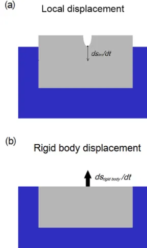
1. First, the topography at a pointrat the surface changes when ice at that point melts (Fig. 1a). Here, the rate of change of topography at a point depends only on lo-cal characteristics of that particular point. For this rea-son, we will call this type of motion “local.” Points on the surface that melt locally move “downwards,” i.e., to lower elevations above sea level.
Figure 1. (a) Local displacement represents the movement of a point on the ice surface as a result of ice melting at that particular point. It is a function only of local ice characteristics at that point. For both local and hydrostatic displacements the positive direction is defined as upwards.(b)Rigid body displacement represents the motion of a floe as a whole in an effort to maintain hydrostatic bal-ance because melting removes mass above or below sea level. Melt-ing above sea level induces an upward rigid body motion of the floe, whereas melting below sea level induces a downward motion.
type of motion the “rigid body” motion. Melting above sea level induces an upward rigid body motion, whereas melting below sea level induces a downward rigid body motion. An ice floe is not a rigid body, but up to its flex-ural wavelength (roughly 30 m on 1.5 m thick ice) we can approximate it as such. As the flexural wavelength is larger than the typical scale of melt ponds (roughly 10 m), the rigid body approximation is likely good. At each point on the ice surface the change in elevation above sea level can be calculated as the sum of these two contributions.
In our model, ponds grow in two ways, “freeboard sink-ing” and “enhanced meltsink-ing”:
1. Freeboard sinking represents the average change in free-board height (average height above sea level of bare ice). In this way the topography of ice above sea level remains unchanged. Freeboard sinking should not be confused with rigid body motion: the average freeboard height always decreases as a response to ice thinning, whereas the rigid body motion can point both upward and downward depending on whether mass is lost above
or below sea level. Both rigid body motion and average local melting contribute to freeboard sinking.
2. Enhanced melting represents the change in the shape of the topography without changing its average height. Ponds can grow in this way if some regions melt faster than average. Therefore, a positive deviation in the local melt rate can grow ponds. Conversely, a negative devia-tion in the local melt rate can slow down or even reverse pond growth. Pond growth only occurs due to topogra-phy changes near sea level. Therefore, deviations from the mean melt rate for points high above the sea level do not influence pond evolution since these points are correlated with points close to sea level only through hydrostatic adjustment, which is determined by the erage melt rates rather than the deviations from the av-erage.
2.2 Equation for the evolution of topography
We now proceed to build the quantitative model of pond evo-lution. Following the above ideas, we divide the total rate of change of vertical position of the pointr on the surface of the ice, ddst(r), into a contribution from rigid body motion,
dsrigid body
dt , and a contribution from local melting,
dsloc
dt (r): ds
dt(r)=
dsrigid body
dt +
dsloc
dt (r). (1)
Ice above sea level (asl) must hydrostatically balance ice below sea level (bsl). We can write this hydrostatic balance as
masl=
ρw−ρi
ρi
mbsl, (2)
wheremasl and mbsl represent the mass of ice above and
below sea level, and ρw and ρi represent the densities of
sea water and pure ice. Throughout the paper we useρw=
1025 kg m−3andρi=916 kg m−3.
The mass above and below sea level can change either be-cause the ice melts or bebe-cause the floe moves as a rigid body, changing the proportion of ice above and below sea level. Therefore, differentiating Eq. (2) and splitting into melt and rigid body contributions, we find
dmmeltasl +dmrigid bodyasl =ρw−ρi
ρw h
dmmeltbsl +dmrigid bodybsl
i
, (3)
where dmmelt/rigid bodyasl/bsl represents changes in mass above and below sea level due to either ice melting or the entire floe floating up or down.
The mass melted above and below sea level after some time dt is
dmmeltasl = −Abi
Fbi
dmmeltbsl = −Amp
Fmp
l dt−A Fbot
l dt, (4b)
wherel=334 kJ kg−1is the latent heat of melting,Fbiis the
total energy flux used for melting bare ice averaged over all bare ice,Fmpis the total energy flux used for melting ponded
ice averaged over ponded ice, and Fbot is the total energy
flux used for melting the ice bottom averaged over the ice bottom.Abi,Amp, andAare the area of bare ice, the area of
melt ponds, and the area of the entire floe, respectively. Since floating up or down does not change the total mass of the ice, mass changes above and below sea level due to rigid body motion are equal with an opposite sign, dmrigid bodyasl = −dmrigid bodybsl . We can express dmrigid body in terms of rigid body displacement of the floe as
dmrigid bodyasl =ρbAbidsrigid body, (5a)
dmrigid bodybsl = −ρbAbidsrigid body, (5b)
whereρb is the bulk ice density. This is the density of sea
ice once all the brine has drained and is always less thanρi.
We assume it to be uniform throughout the vertical ice col-umn, but we discuss the effects of vertical variations inρbin
Sect. 7.2.
Substituting Eqs. (4) and (5) into Eq. (3), solving for dsrigid body, and differentiating with respect to time, we find
the rate of change of surface topography due to rigid body motion to be
dsrigid body
dt =
" ρi ρw Fbi lρb # − "
ρw−ρi
ρw Amp Abi Fmp lρb # − "
ρw−ρi
ρw A Abi Fbot lρb # . (6)
The three terms in large square brackets correspond to to-pography change due to bare ice melting, ponded ice melting, and ice bottom melting. Rigid body motion depends only on spatially averaged energy fluxes, which in turn depend on parameters such as the average insolation on the floe, the av-erage albedo, and the avav-erage longwave, sensible, latent, and bottom heat fluxes. If bare and ponded ice melt only from en-ergy absorbed by the upper surface of the ice, the fluxesFbi
andFmpcan also be written in terms of albedo as
Fbi=(1−αbi)Fsol+Fr, (7)
Fmp=(1−αmp)Fsol+Fr, (8)
where αbi and αmp are the average albedos of bare and
ponded ice,Fsolis the solar flux, andFris equal to the sum of
net longwave, net sensible, and net latent heat fluxes. This pa-rameterization neglects light transmission and assumes that all of the energy is deposited in the surface. Much of the variation in albedo of ponded ice is due to the fact that the pond bottom is partially transparent, and energy is deposited
in the ocean instead of directly in the ice. However, this does not make much difference in our model since the energy de-posited in the ocean is likely used for melting ice below sea level anyway.
Local displacement, dsloc, quantifies how much the ice
sur-face topography changes as a result of local melt. We can de-termine the local melt rate fromFsurf(r), the flux of energy
used for melting the ice surface at a pointr: dsloc
dt (r)= − Fsurf(r)
lρb
, (9)
where the positive direction is defined as upwards. The lo-cal flux depends on parameters such as the lolo-cal albedo, the local insolation, the local longwave, sensible and latent heat fluxes, and the angle between ice and incoming radiation at that point.
The fluxFsurf(r)averaged over all the points on the
sur-face of the ice above sea level equalsFbi:
< Fsurf(r) >=Fbi, (10)
where< . . . > represents averaging over all the points on bare ice. For this reason, we will parameterize the rate of local melting as
dsloc
dt (r)= −k(r) Fbi
lρb
, (11)
wherek(r)is a nondimensional number that quantifies the deviation of the melt rate at the pointr from the mean melt rate of the bare ice surface, which depends on the detailed conditions of ice and its environment. The parameterkcould be either greater than or less than 1. Here we will takekto be constant in time, but in reality it need not be. Finally, accord-ing to Eq. (1) we add Eqs. (6) and (11) to get the equation for the evolution of the bare ice topography. We express this in terms of melt pond fraction,x≡Amp
A : ds
dt(r)= −
"
(k(r)−1)Fbi lρb
#
−
ρ
w−ρi
ρw
1
lρb
Fbi+
x
1−xFmp+
1 1−xFbot
. (12) Here, we split the equation into two terms, enclosed by the square brackets. The first term represents the local deviation from the average surface melt rate, which changes the general shape of the topography while preserving its average height above sea level. We identify this term with enhanced melt-ing. The second term represents a global shift of the average elevation above sea level due to freeboard sinking.
In this way, the topographic evolution equation can be split into two terms, enhanced melting and freeboard sinking: ds
dt =
dsem
dt +
dsfs
dt , (13)
wheredsem
dt and
dsfs
2.3 Model for the evolution of pond coverage
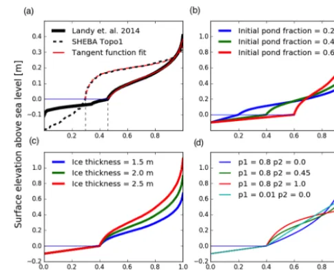
We now need to relate the vertical displacements near the sea level to the change in area of the melt ponds. To this end we define the hypsographic curve,s(xh), which relates the ele-vation above sea level,s, to the percent of ice surface below that elevation,xh (Fig. 2). Such curves have been measured and reported on several occasions (e.g., Fig. 8 of Eicken et al., 2004, or Fig. 8 of Landy et al., 2014). If the ice is highly permeable, the melt pond fraction, x, can be inferred from a hypsographic curve as the intersection of sea level with the curve. Since ponds are hydraulically connected with the ocean, the average freeboard height of bare ice,h, depends on the pond fraction. The average freeboard height, h, can be expressed in terms of the ice thickness H and the pond fraction as
h=ρw−ρi
ρw
H
1−x. (14)
Here, the average freeboard height is defined as the eleva-tion of the ice surface above sea level averaged over bare ice. For two ice floes of the same thickness, the one with higher pond coverage will also need to have a higher average free-board in order to maintain hydrostatic balance.
The above sea level part of every measured hypsographic curve we tested can be fit relatively well with a tangent func-tion (Fig. 2a, red line). We will assume that this fit holds for a wide range of different sea ice floes and use it to initial-ize our model with different physical parameters. We give the exact form of this function in Appendix A (Eq. A1). To get a hypsographic curve for a particular initial pond frac-tion,xi, and ice thickness,H, we set it to zero at the initial pond coverage,s(xh=xi)=0, and rescale it vertically to get a freeboard that hydrostatically balances the floe. The topog-raphy below sea level is not important for the evolution of pond coverage if the pond coverage grows, and we replace it with a straight line.
We show several curves for different initial ice thickness and initial pond coverage in Fig. 2b and c. We note that the initial pond fraction, xi, corresponds to the pond fraction when ice first becomes permeable. Once we choose xi and H, the tangent function Eq. (A1) has only two unconstrained parameters, p1 and p2, that determine the exact shape of
the curve. Knowing additional physical parameters, such as ice roughness, we can constrain additional parameters of this curve. Throughout this paper we will mostly usep1andp2
that fit the measurements of the hypsographic curve made by Landy et al. (2014) for 25 June 2011 or the measure-ments made during the SHEBA mission along the topogra-phy profile “1” on 10 July 1998. However, when examining the effects of sea ice roughness, we will vary these param-eters to get curves of different shape. Several examples of hypsographic with differentp1andp2are shown in Fig. 2d.
In the case of pure freeboard sinking the overall shape of the hypsographic curve does not change as the ice melts.
In-Figure 2.Hypsographic curves showing the percentage of the sea ice surface that is lower than a particular elevation. Pond coverage on highly permeable sea ice can be inferred from here as the in-tersection of sea level (horizontal blue line) with the hypsographic curve.(a)A hypsographic curve measured by Landy et al. (2014) on 25 June 2011 (solid black line) and a hypsographic curve mea-sured during SHEBA along a 100 m long “topography profile 1” on 10 July 1998 (black dashed line). The vertical dashed lines rep-resent the pond coverage, assuming that ice is permeable. The red line represents a fit to the part of the hypsographic curve above sea level with a tangent function, Eq. (A1).(b)Adjusted hypsographic curves for different initial pond coverage and the same ice thick-ness.(c)Adjusted hypsographic curves for the same initial pond coverage and different ice thickness.(d)Hypsographic curves for different shape parameters,p1andp2, defined and discussed in
Ap-pendix A, Eq. (A1). Parameterp1controls the amount of curvature,
whilep2controls the position of the inflection point of the tangent
function.
stead the whole curve is shifted following a displacement of dsfs(Fig. 3a). We can calculate the resulting change in pond
coverage as dx
dt =
dxh ds (x)
dsfs
dt , (15)
where dsfsis the vertical displacement of the bare ice
topog-raphy due to freeboard sinking (as determined by the second term in Eq. 12), anddxh
ds (x)is the change in pond fraction for a vertical shift of the ice surface of dsfswhen the pond
frac-tion is equal tox. It is equal to the reciprocal of the derivative of the hypsographic curve,s(xh), evaluated atxh=x. Sub-stitutingdsfs
dt from Eq. (12) we find dx
dt =
dxˆh dsˆ (x)
Sbi+Smp b
x
[ 1−x
+Sbot
1 [ 1−x
, (16)
wherebx≡ x
xi and 1[−x≡ 1−x
1−xi are the pond and bare ice
fractions normalized by the initial pond and bare ice frac-tions, anddxˆh
dsˆ(x)≡
h
1−xi dxh
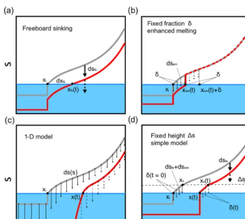
Figure 3.Explanation of different models of pond growth. Models evolve a hypsographic curve,s(xh), above sea level to find the pond coverage evolution. Evolution of the hypsographic curve below sea level is not relevant for pond growth and, apart from the 1-D model, is not captured well in these models.(a)Freeboard sinking shifts the entire hypsographic curve downward following a displacement of dsfs. (b) Enhanced melting acts on a constant ice fraction,δ,
and there is no freeboard sinking. The hypsographic curve changes only betweenxh=xandxh=x+δand remains unchanged other-wise. After a time1t= s(x+δ)
dsem/dt pond coverage grows byδ. The 0-D model, Eq. (26), assumes that the total pond evolution is the sum of pond evolution due to such enhanced melting and freeboard sinking (panela).(c)The 1-D model prescribes a melt rate at each point on the hypsographic curve as a function of height above sea level,
ds
dt(s).(d) A simplified model that assumes both freeboard sink-ing and enhanced meltsink-ing (Appendix B). Enhanced meltsink-ing occurs only below height1s. After some time, the fraction of ice affected by enhanced melting,δ, becomes constant, meaning that a constant fraction model (panelb) and a constant height model are equivalent ifδand1sare related appropriately.
of the hypsographic curve. We have defined the strengths of pond growth by freeboard sinking due to melting bare, ponded, and ice bottom,Sbi,Smp, andSbot, as
Sbi≡
(1−xi)2Fbi
H lρb
, (17a)
Smp≡
(1−xi)xiFmp
H lρb
, (17b)
Sbot≡
(1−xi)Fbot
H lρb
. (17c)
The nondimensional factorsbx,1[−x, and dxˆh
dsˆ (x)are
cho-sen to be of the order unity, so thatSbi,Smp, andSbotcontrol
the strengths of pond growth by melting bare ice, melting
ponded ice, and melting ice bottom. The reciprocals of the strengths represent the timescales of the growth modes.
The set of parameters needed to describe pure freeboard sinking can be further reduced by rewriting Eq. (16) as dx
dt =
dxˆh dsˆ (x)
S1 b
x
[ 1−x
+S2
1 [ 1−x
, (18)
whereS1≡Smp−xiSbi/(1−xi)andS2≡Sbot+Sbi/(1−xi) represent a minimal set of parameters needed to describe pure freeboard sinking. However, these parameters do not have a clear physical interpretation, and we will henceforth focus only onSbi,Smp, andSbot.
Next we need to consider the contribution from enhanced melting. Before doing so we need to make some assumptions about the nature of enhanced melt. There are multiple phys-ical processes that can cause the melt rate to deviate from the mean. One process that stands out as being particularly important is albedo decrease due to ice wetting: ice close to sea level will likely be wet and therefore have a lower albedo compared to ice higher up. The deviation from the mean melt rate in this case depends primarily on the height above sea level. Another potential contribution to height-dependent en-hanced melt may effectively come from random fluctuations in the melt rate around the average: ice near the sea level has a higher probability of falling below sea level due to random fluctuations than ice higher up. After falling below sea level, ice becomes ponded, melts faster, and is unable to return to its previous position. Other processes, such as lateral melt, may not depend on height above sea level, but for now we neglect this possibility (see Sect. 7.1 for discussion).
Because of the processes described above, we will assume that the deviation from the mean melt rate,k(r)−1, depends only on height above sea level,s. In this scenario, we need to consider enhanced melting together with freeboard sink-ing, as freeboard sinking constantly supplies new ice to low elevations to be affected by enhanced melting. Effects of en-hanced melting and freeboard sinking can be approximately separated if, instead of height dependence, enhanced melt-ing is constrained to act on a fixed fraction of bare ice. In this case, a constant fraction of bare ice that would experi-ence enhanced melting would evolve, at least approximately, independently of freeboard sinking.
Therefore, we will consider two cases of enhanced melt-ing. Firstly, we will consider a height-dependent enhanced melting. In particular, we will assume thatk(0< s < 1s)≡
ifδis appropriately chosen, a height-dependent model and a fixed fraction model become equivalent. Therefore, we will first solve a model assuming a fixedδand no freeboard sink-ing and then relate it to a fixed 1s model by choosing the appropriateδ.
We note that the assumption thatk(r)=1 high above the sea level and k(r) >1 near the sea level is strictly not true since averaged over all of bare ice k(r) needs to equal 1. However, it is approximately true if1sorδ are small, such that the area wherek(r)6=1 is small compared to the total area of bare ice. Also, we have assumedk(r)=1 high above the sea level without loss of generality, since deviations from the mean melt rate high above the sea level are not important, as only ice close to sea level may become ponded.
Now we proceed to consider the case of “pure enhanced melting” that assumes a fixed fraction of the ice, δ, melts, and there is no freeboard sinking (Fig. 3b). If there is no to-pographic variation above sea level, and the entire ice floe above sea level has the same height, h, the pond coverage would grow by δ after a time1t= h
dsem/dt, where dsem/dt
is the rate of change of topography due to enhanced melting as determined by the first term of Eq. (12). Therefore, the pond growth rate in this case would be 1x1t =δ
h
dsem
dt . If there is non-negligible topography above sea level described by the hypsographic curve, the time1t it takes for pond coverage to grow byδwould be1t=s(xh=x+δ)
dsem/dt . Here,s(xh=x+δ)
is the original hypsographic curve evaluated at xh=x+δ. We will assume this expression generally holds for enhanced melting. Thus, we arrive at the expression for pond growth due to pure enhanced melting with fixedδ:
dx
dt = δ s(x+δ)
dsem
dt . (19)
Ifδ is small compared to the variation in the hypsographic curve, we can substitutes(x+δ)withs(x). This is only not justified near the beginning of the melt, whens(x)≈0. Sub-stituting dsem
dt from Eq. (12) we find dx
dt =Sem
1
ˆ
s(x+δ), (20)
where s(x)ˆ ≡s(x)
h is the nondimensional hypsographic curve, and the strength of the enhanced melting,Sem, is
de-fined as
Sem≡
ρw
ρw−ρi
(1−xi)δ(k−1)Fbi
H lρb
. (21)
Ultimately, however, our goal was to describe the height-dependent enhanced melting. In Appendix B, we showed that such a model can be approximated with a fixed fraction model, if we appropriately relateδ and1s. Here we simply state the result:
δ= ρw
ρw−ρi
21s(1−xi)2 3H1+dsem
dsfs
. (22)
Here, dsem
dsfs represents the ratio of the topographic rate of
change due to enhanced melting to freeboard sinking and is given by
dsem
dsfs
= ρw
ρw−ρi
|Fbi|(k−1)
|Fbi| +1−xixi|Fmp| + 1 1−xi|Fbot|
, (23)
where |F| are the representative values of energy fluxes, e.g., their time averages. Therefore, the strength of height-dependent enhanced melting becomes
Sem=
ρ
w
ρw−ρi
221s(1−x
i)3(k−1)Fbi
3H2lρ b
1+dsem
dsfs
. (24) We have made a number of assumptions in deriving the expression for enhanced melting. Below we compare this model to a more complicated “1-D” model and show that all these assumptions are justified. We also show that if the function describing the local melt rate,k(s), has a nontriv-ial dependence on height above sea level, parameterSemis
better replaced with a parameter:
< Sem>≡
ρw ρw−ρi
2
2(1−xi)3Fbi 3H2lρ
b ∞ Z
0
k(s)−1 1+dsem
dsfs(s)
ds. (25)
In this way, we have separated the effects of freeboard sinking and enhanced melting. Finally, we will assume that contributions from freeboard sinking and enhanced melting can be added independently. Therefore, we solve Eq. (16) for pure freeboard sinking and Eq. (20) for enhanced melt-ing independently, and we add them together to get the full evolution of pond coverage,x(t ):
x(t )=xfs(t )+xem(t )−xi, (26)
wherexfs(t )andxem(t )are solutions to Eqs. (16) and (20),
both forced using the same parameters and initialized with the same initial pond fraction xi. This concludes the 0-D model.
Equation (26) represents a sum of solutions to two simple ordinary differential equations, in which the rate of change of pond fraction depends on the pond fraction. Here, we have reduced the number of parameters from the original 10 (H,
xi,ρb,Fbot, Fsol,Fr, αbi,αmp,k, and1s) to 4 (Sbi,Smp,
Sbot, andSem). The strengths of freeboard sinking,Sbi,Smp,
andSbot, depend only on the parameters that are available
in GCM simulations and are relatively easily measured in observational studies. The enhanced melting strength,Sem,
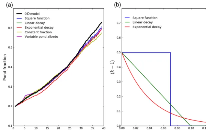
Figure 4. (a)A comparison between pond evolution in the 0-D model and the 1-D model. The black curve represents the 0-D model. The blue, green, and red curves represent the 1-D model for different functionsk(s)shown in panel(b). These different functions were chosen such that the integral parameter< Sem>(Eq. 25) is the same as for the 0-D model. The yellow curve represents the 1-D model where
enhanced melting acts on a constant fraction of bare ice,δ, chosen according to Eq. (22). The magenta curve represents the 1-D model with pond albedo varying with depth. There is significant agreement between all of the curves, suggesting that the simplifications made in the simple model were justified. Since including variable pond albedo does not change the pond evolution significantly, this detail can be neglected when estimating the pond coverage on permeable ice.(b)The blue, green, and red lines represent functionsk(s)−1 used to run the 1-D model.
2.4 Testing the model
In order to test the assumptions we made to simplify the model, we have developed a “1-D” model in which we ex-plicitly determine pond evolution when both freeboard sink-ing and enhanced meltsink-ing are happensink-ing simultaneously. Apart from resolving the melt rates in one dimension, the underlying assumptions for the 1-D model are essentially the same as for the simple model. For this reason, we simply give an outline for this model, without discussing it in much detail.
In the 1-D model, we evolve the hypsographic curve by prescribing a melt rate, dsloc, to each point on the
hyp-sographic curve depending on the height above sea level (Fig. 3c). The hypsographic curve high above sea level melts at a uniform rate, whereas the hypsographic curve slightly above sea level melts at an enhanced rate. Parts of the curve below sea level melt at a uniform rate determined by the flux used for melting ponded ice, Fmp. Finally, hydrostatic
ad-justment is calculated by finding the ice thickness directly at each time step and placing the floe in hydrostatic balance. The evolution of pond coverage obtained from this model is shown in Fig. 4a. The comparison with the simple 0-D model is excellent.
The 1-D model allows us some freedom to test the detailed assumptions of the 0-D model. First, we can test how the functional form ofk(s)affects the pond evolution (Fig. 4b).
The functionsk(s)were chosen such that they all have the same integral parameter< Sem>defined in Eq. (25).
Fig-ure 4a shows that in each of these cases the evolution of pond coverage proceeds nearly identically. Second, we can test the difference between an assumption that enhanced melting acts below a constant height1sand an assumption that enhanced melting acts on a constant fraction of ice,δ. The yellow line in Fig. 4a shows that if δ and1s are chosen according to Eq. (22), both assumptions yield very similar results. Finally, we can test the effects of varying pond albedo. In reality pond albedo decreases as the ponds deepen. We assume a depen-dence of pond albedo on pond depth reported in Table VII of Morassutti and Ledrew (1996) for mean broadband albedo. The magenta line in Fig. 4a shows that allowing for pond albedo to vary has a negligible effect on pond evolution.
3 A 0-D model can approximate observations well using realistic parameters
In Fig. 5, we compare the results from our model to obser-vations made on a 200 m long albedo line during SHEBA (red line). Ice along the albedo line was level multiyear ice, but the ponds drained to sea level after some time, which makes them amenable to our model (Perovich et al., 2003). The pond coverage along the albedo line dropped to a mini-mum around the end of June. Therefore, we choose to model only the period after 1 July. In order to keep the albedo line pristine, no thickness measurements were made. However, relatively close to the albedo line, topography measurements were made along a level multiyear ice profile roughly ev-ery 10 days. After approximately 10 July, ponds along the topography profile also drained to sea level. We show the topography profile pond coverage in blue dots (we have ar-tificially subtracted 0.05 from the pond coverage to facilitate comparison with the pond coverage along the albedo line). The pond coverage both along the topography profile and along the albedo line follows roughly the same trend, sug-gesting that the physical parameters driving the pond evolu-tion in the two places are likely similar. Based on the average freeboard height, we estimate the ice thickness on 10 July to be roughly 1.4 m along the topography profile, meaning that on 1 July ice thickness was around 1.6 m. Therefore, we assume the same thickness for the ice along the albedo line and use a hypsographic curve corresponding to the one measured along the topography profile on 10 July (Fig. 2a, dashed line). In order to run our model, we use the melt rates of bare ice, ponded ice, and ice bottom measured directly us-ing ablation stakes durus-ing SHEBA (Perovich et al., 2003). We choose a realisticρb=850 kg m−3(Timco and
Frederk-ing, 1996). We have no way of directly constraining the pa-rameters1sandkthat control the strength of enhanced melt-ing. Therefore, we treatSemas a fitting parameter. Choosing
Sem=0.22 month−1 fits the observations well by eye. This
value can be obtained using1s=15 cm andk=1.7, which likely fall at the upper end of the range of reasonable values for these constants (see Sect. 4 for a discussion on 1sand
k). Such a high value ofSem can be explained by a
signifi-cant contribution from lateral melting.
The full black line in Fig. 5 represents a solution to the full Eq. (26). The agreement between model and observa-tion is excellent, with a maximum discrepancy of 3 % pond coverage at the end of the melt season. The dashed black line represents the contribution to pond growth due to free-board sinking, whereas the dotted line corresponds to en-hanced melting. Almost all pond growth in this case is due to enhanced melting. This is due to ice topography. On mul-tiyear ice, meltwater typically collects in depressions formed by ponds in previous years. The topography created in this way is highly bimodal, and, after drainage, ponds typically have steep walls. Bare ice topography, in contrast, is rela-tively smooth, preventing new pond formation. This is
ap-parent in the hypsographic curve we used. Such a topography inhibits freeboard sinking, and pond coverage grows mostly by enhanced melting acting near the pond sidewalls, growing the existing ponds. In addition to height-dependent enhanced melting we introduced in the previous section, in this case there is likely a significant contribution from lateral melting as well. This contribution helps explain the high value ofSem
we had to choose to get a close agreement between our model and observations. First-year ice topography, in contrast, per-mits ample pond growth through freeboard sinking. Observa-tions suggest that on first-year ice ponds grow primarily due to freeboard sinking (Polashenski et al., 2012; Landy et al., 2014).
4 Numerical solutions
We now solve Eq. (26) numerically to gain intuition about the behavior of our model. We use a set of realistic parameters we will henceforth refer to as the “default parameters.”
For shortwave, longwave, latent, and sensible heat fluxes, we use values inferred by Skyllingstad et al. (2009) using hourly measurements from the SHEBA mission. We use the bottom heat flux inferred from measurements of ice bottom ablation during the SHEBA mission (Perovich et al., 2003). The albedo of bare ice can vary between 0.5 and 0.7 (Hane-siak et al., 2001), while the albedo of melt ponds can vary be-tween 0.1 and 0.6, depending on pond depth and conditions of ice at the pond bottom (Morassutti and Ledrew, 1996; Per-ovich et al., 1998; PerPer-ovich, 1996). Here we prescribe a de-fault bare ice albedo of 0.55 and a default pond albedo of 0.2. We use a realistic bulk ice density ofρb=850 kg m−3
(Timco and Frederking, 1996). We use an initial ice thickness of 1.5 m and use the first-year ice topography measured by Landy et al. (2014) adjusted for the prescribed ice thickness and initial pond fraction (usuallyxi=0.2). We will assume enhanced melting is entirely due the albedo dependence on height above sea level. Some preliminary results based on field measurements of bare ice albedo on first-year ice sug-gest that albedo changes from around 0.3 near sea level to around 0.55 at a height of around 10 cm above sea level, af-ter which the correlation between albedo and surface eleva-tion tapers off (Chris Polashenski, personal communicaeleva-tion, 2017). Using such an albedo and the average values of short-wave, longshort-wave, latent, and sensible heat fluxes, we can esti-mate the rate of melt as a function of height above sea level,
k(s)=F (s)
Fbi
. Using Eq. (25), we can then find the integral pa-rameter< Sem>. We choose1s=6 cm andk=1.7 to
cor-respond to the same integral parameter. We should note that there is significant scatter in the data, and measurements cor-respond to only one study. Therefore, this is a rough estimate of enhanced melting, but it is likely of the correct order of magnitude.
Figure 5.A comparison between measurements of pond fraction made during SHEBA along the albedo line (red line), along a to-pography profile (blue dots), and our model (black line). The blue dots have been shifted downward by 0.05 to make a more obvious comparison between albedo line and topography profile trends. The black dashed line is the contribution to our model from freeboard sinking and the black dotted line is the contribution from enhanced melting. Ponds grow almost entirely due to enhanced melting as a result of the steep topography of multiyear ice.
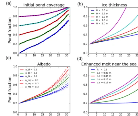
when the initial pond coverage is lower, and the pond evo-lution curves cluster together as time progresses. This is be-cause lower initial pond coverage corresponds to lower initial freeboard height, making the pond growth more rapid. The dashed line corresponds to the solution using the fluxes time-averaged over the 30-day run. The solutions using the aver-aged fluxes are very similar to the ones using time-varying fluxes, meaning that daily and even monthly variations in the forcing have little effect on pond growth. This insensi-tivity to short timescale variations in the forcing means that pond coverage evolution may be faithfully represented in the large-scale models, as it would not be affected by the coarse timescales of those models. Henceforth, we will use the time-averaged fluxes.
A larger ice thickness means a higher freeboard. For this reason, ponds grow more slowly on thicker ice. Because the pond growth rate is inversely proportional to ice thickness, pond coverage is more sensitive to variations in ice thickness when the ice is thin (Fig. 6b). In Fig. 6b we see that a 0.5 m difference in the initial ice thickness (between a floe 1.5 m and a floe 2 m thick) can mean a 20 % difference in pond coverage at the end of the melt season.
Figure 6c shows the dependence of pond coverage on albedo. A variation of 0.1 in bare ice albedo has a much larger effect on pond evolution than the same change in pond albedo. The reason is that melting ponded ice only affects pond coverage through downward rigid body motion of the floe, whereas melting bare ice grows the ponds through both
Figure 6.Numerical solutions to Eq. (26) with parameters varied around the defaults described in the text.(a)Varying initial pond coverage. Solid lines represent solutions using full time-varying fluxes, while dashed lines represent solutions using time-averaged fluxes. The two solutions are very similar, so we subsequently use only the time-averaged fluxes. (b) Varying ice thickness. Ponds grow slower on thicker floes.(c)Varying pond and bare ice albedo. Different colors represent different bare ice albedos, and full, dot-ted, and dashed lines represent different pond albedos. A change in bare ice albedo has a much larger effect on pond fraction than the same change in pond albedo.(d)Varying the1sandk. Fork=0.8, the ponds shrink. However, pond evolution fork <1 is not repre-sented well in our model, so this curve serves only as an illustration.
enhanced melting and freeboard sinking. Furthermore, when pond coverage is low, rigid body motion due to ponded ice melting is less efficient than that due to bare ice melting be-cause it is proportional to melt pond fraction.
The parameters controlling the strength of enhanced melt-ing are the least constrained parameters in our model. In Fig. 6d we show the dependence of pond evolution on the height below which enhanced melting is active,1s. Explor-ing a range of realistic values for1s, 0< 1s <15 cm, we find that the pond fraction at the end of the melt season can vary by about 30 %. This difference would be larger if we chose a smaller ice thickness. The effects of changingkare relatively small, so long askis large enough (not shown). For example, using current parameters, pond coverage evolution becomes fairly insensitive tokwhenk >1.5. Smaller values ofk, however, can significantly impact pond evolution. Ifk
is sufficiently smaller than 1,Semcan become negative and
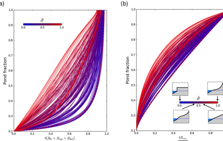
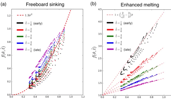
Figure 7.Exploring the effects of sea ice roughness.(a)Pond evolution due to pure freeboard sinking for hypsographic curves with different shape parametersp1andp2. Thexaxis shows nondimensional timetˆ=
t (Sbi+Smp+Sbot)
1−xi . Color represents normalized roughness,σˆ, with
blue colors corresponding to smallσˆ and red colors corresponding to largeσˆ. Thick red solid line represents pond evolution on the measured first-year ice hypsographic curve, and the thick red dashed line represents pond evolution on the measured multiyear ice hypsographic curve. All else equal, rougher ice has a larger pond fraction.(b)Pond evolution due to pure enhanced melting for hypsographic curves with different shapes. Thexaxis shows nondimensional timetˆ= t Sem
1−xi. Cartoon examples of hypsographic curves and their approximate positions along
theσˆ axis are also shown.
becomes invalid in this case, and the blue curve in Fig. 6d serves therefore simply as an illustration.
5 Pond evolution is slower on smoother ice
The evolution of pond coverage in our model depends on the detailed shape of the hypsographic curve, which is not captured by the strengths of freeboard sinking and enhanced melting. As we show below, pond coverage is sensitive to such details and in particular to ice roughness. Below we will introduce the “effective strengths”, S∗, which approxi-mately capture the effects of roughness and allow us to esti-mate mean pond coverage after a period of time. Using effec-tive strengths, we will demonstrate how multiyear ice topog-raphy suppresses pond growth by freeboard sinking, while first-year ice topography permits it.
In the tangent function parameterization, Eq. (A1), the ex-act shape of the hypsographic curve is determined by param-etersp1andp2. Here, we will not discuss these parameters
individually but will rather focus on often measured bare ice roughness,σ, defined as the standard deviation of surface el-evation of ice above sea level:
σ ≡
R1 xis
2(x
h)dxh 1−xi
−h2
!
1 2
. (27)
We will use the nondimensional form of bare ice roughness, defined asσˆ ≡σ
h. Typically, a concave hypsographic curve (e.g., Fig. 2d, red curve) will have a smallσˆ, whereas a con-vex hypsographic curve (e.g., Fig. 2d, blue curve) will have a highσˆ.
During the permeable stage, all else equal, ponds will grow more rapidly on rougher ice, since a larger fraction of ice is close to sea level. This is not true on impermeable ice, as meltwater filling deep topographic lows on rough ice will cover a smaller area relative to the same amount of meltwa-ter filling shallow topographic lows on smooth ice. For this reason, the initial pond coverage will likely be smaller on rougher ice due to a smaller pond coverage during the imper-meable stage.
Figure 7 shows the pond coverage evolution due to pure freeboard sinking (Fig. 7a) and pure enhanced melting (Fig. 7b) for hypsographic curves with different parameters
p1andp2and all other parameters kept constant. For each
choice ofp1andp2, we find the normalized bare ice
We wish to quantify the effect of roughness by its impact on the mean pond coverage. In particular, we hope to find the “effective strengths”,S∗(σ )ˆ , which include the roughness ef-fects and allow us to easily estimate the average pond cover-age after some timet:
< x(t ) >≈1
2S
∗
t+xi, (28)
where < x(t ) >≡
Rt
0x(t )dt
t . Effective strengths are propor-tional to strengths of freeboard sinking and enhanced melting we derived in Sect. 2.3. In general they themselves may de-pend on time and are indede-pendent of time only if pond cover-age evolution is linear,x(t )=St+xi, in which caseS∗=S, whereSis eitherSfs≡(Sbi+Smp+Sbot)in the case of
free-board sinking orSemin case of enhanced melting.
In Appendix C, we describe the procedure to estimate the effective strengths as functions of nondimensional roughness and time. Here, we only state the result:
Sfs∗ ≈h1.3σˆ2i Sbi+Smp+Sbot
, (29a)
Sem∗ ≈
"
1+ 2
p
ˆ
tem
−3
2 !
ˆ
σ
#
Sem, (29b)
whereSfs∗ is the effective strength of freeboard sinking,Sem∗
is the effective strength of enhanced melting, andtˆem≡ Semt
1−xi
is the nondimensional time of pond evolution due to en-hanced melting. The terms in square brackets represent the corrections due to roughness. If both freeboard sinking and enhanced melting occur simultaneously the total effective strength is the sum of these two, S∗=Sfs∗+Sem∗ . Knowing the effective strengths allows us estimate the mean pond cov-erage after a period of time without having to run the model. Roughness has a different effect on freeboard sinking and enhanced melting. Freeboard sinking is roughly indepen-dent of time and proportional to the square of nondimen-sional roughness. Therefore, it is very sensitive to variations in roughness: doubling the ice roughness roughly quadru-ples the mean pond coverage due to freeboard sinking after some time. Enhanced melting depends roughly linearly on roughness. However, as roughness tends to zero, the effec-tive strength remains nonzero, Sem∗ (σˆ →0)→Sem.
There-fore, ponds on smooth ice grow primarily due to enhanced melting. Effective strength also depends on the nondimen-sional time,tˆ, and is higher and more sensitive to variations
in roughness early in the melt season.
Multiyear ice topography shown in Fig. 2a, dashed line, hasσˆ ≈0.25 and is significantly smoother than first-year ice topography shown in Fig. 2a, solid line, which hasσˆ ≈0.55. From Eq. (29) it follows that freeboard sinking on multiyear ice is roughly 5 times less efficient in growing the ponds than on first-year ice.
6 Analyzing the 0-D model yields useful insight into factors influencing the pond evolution
Extracting the dependence of a desired property on physical parameters and understanding its scaling is the main strength of our model. These types of relationships would be difficult to obtain in a more complex model.
The parametersSbi∗,Smp∗ ,Sbot∗ , andSem∗ control the mean rates of pond growth by melting different regions of ice. Roughly, they represent the amount of pond growth per unit time by freeboard sinking due to melting bare ice, freeboard sinking due to melting ponded ice, freeboard sinking due to melting ice bottom, and enhanced melting. Knowing these parameters allows us to estimate mean pond coverage after a period of time with significant accuracy without having to run the numerical model. Moreover, analyzing them can yield useful insight into the behavior of melt ponds under general circumstances.
We can estimate the change in magnitude of the strength of each of the growth modes when a physical parametersp
changes by1pas
1Si∗=∂S
∗
i
∂p 1p, (30)
where 1Si∗ is the change in magnitude of the effective strength of the ith growth mode. This equation holds so long as the change in the physical parameter is not too large. A change in pond growth rate can then be estimated as 1S∗=P
i1Si∗. Then, using Eq. (28), we can roughly estimate a change in mean pond fraction, 1 < x >, after some time,1t, following a change in physical parameter,p, as 1 < x >≈1
21S
∗1t. This provides a means to estimate
changes in mean pond coverage under different environmen-tal conditions.
6.1 Ponds are more sensitive to changes in bare ice albedo than changes in pond albedo
We will illustrate the use of effective strengths using an ex-ample where we vary the ice and pond albedos. If the bare ice albedo changes by1αbi, the change in growth rate would
be roughly
1S∗=
S
∗ bi+
ρw−ρi
ρw (dsem/dsfs)
2+(k−1)
1+dsem
dsfs
(k−1)
Sem∗
×Fsol
Fbi
1αbi≈ −0.9
1
If the melt pond albedo changes by1αmp, the change in
growth rate would be roughly
1S∗= −
S
∗
mp+
(ρw−ρi) xi(dsem/dsfs)2Fmp
ρw
1+dsem
dsfs
(k−1)(1−xi)Fbi
Sem∗
× Fsol
Fmp
1αmp≈ −0.2
1
month1αmp. (32)
It follows from these estimates that after a month the mean pond fraction would differ by roughly 4.5 % for a bare ice albedo difference of 0.1 and by around 1 % for a pond albedo difference of 0.1. Therefore, variation in pond albedo affects pond evolution roughly 5 times less than variation in bare ice albedo. This explains our observation from Fig. 6c that pond evolution is much more sensitive to variations in bare ice albedo than to variations in pond albedo. In this way, we also extract the dependence of sensitivity on physical param-eters. A major difference between the two sensitivities is their dependence on the initial pond coverage: the sensitivity to pond albedo is proportional toxi, whereas the sensitivity to bare ice albedo is proportional to 1−xi. In the above ex-ample we used xi =0.2, which explains most of the large difference between the two sensitivities. If the pond cover-age were higher, variations in the pond albedo could become more important than variations in bare ice albedo. For exam-ple, assuming no enhanced melting, the sensitivity to pond albedo would become greater than the sensitivity to bare ice albedo at 50 % pond coverage1S
∗
mp 1S∗
bi
= xi 1−xi
1αmp 1αbi
.
6.2 Under global warming, pond feedback could lead to significant ice thinning
We now use the effective strengths to roughly estimate the impact of global warming on the pond coverage. At high lat-itudes, feedbacks due to changes in albedo, the atmospheric lapse rate, and clouds can amplify the forcing due to global warming (Holland and Bitz, 2006). For this reason forcing at high latitudes is generally larger than direct radiative forcing due to an increase in CO2concentration. In a global
warm-ing scenario, the pond growth rate would increase because the ice melts faster but also because ice at the beginning of the melt would be thinner. We can emulate a global warming scenario by increasing the fluxFrby a certain amount,1Fr, and by assuming that the initial ice thickness decreases by
1H≡ ∂H
∂Fr1Fr, where
∂H
∂Fr is the ice thinning per 1 W m −2
of warming. Therefore, we split the change in pond growth rate due to global warming, 1S∗, into a contribution from direct forcing, 1SF∗, and a contribution from ice thinning,
1SH∗. Using the above formalism, we find
1SF∗ ≡X
i ∂Si∗ ∂Fr
1Fr
= "
Sbi∗
Fbi +S ∗ mp Fmp +
ρw−ρi
ρw (dsem/dsfs)
2+(k−1)(1−x
i)
(1+dsem
dsfs)(k−1)(1−xi)
Sem∗ Fbi #
1Fr
≈ 0.5 %
W m−2×month1Fr, (33a)
1SH∗ ≡X
i ∂Si∗
∂H ∂H ∂Fr
1Fr
= −Sbi∗+Smp∗ +Sbot∗ +2Sem∗ 1 H
∂H ∂Fr
1Fr
≈ 1.9 %
W/m2×month1Fr, (33b)
1S∗≡1S∗F+1SH∗ ≈ 2.4 %
W m−2×month1Fr. (33c)
The numbers in Eq. (33) were obtained using the default val-ues of the parameters, and∂F∂H
r = −0.05 m
3W−1roughly
es-timated using the Eisenman and Wettlaufer (2008) model. This means that after a month’s growth global warming would increase mean pond coverage by roughly 1.2 % per 1 W m−2of warming. Nearly half of this increase in the mean pond coverage comes from an increase in the strength of en-hanced melting due to ice thinning. Simulating a 30-day melt numerically using our model predicts an increase in mean pond coverage with forcing at a rate of 1.5 % per 1 W m−2 of warming for small forcing (1Fr≈0), which confirms the approximate validity of our linearization. For larger forcing, the sensitivity of pond coverage to forcing increases because the ice thins. Our linearized estimate, Eq. (33), also gives the dependence of the sensitivity on physical parameters. In a likely scenario where the forcing is around 10 W m−2, our
es-timate predicts that after a month mean pond coverage would increase by around 15 %, which corresponds to around 12 cm of ice thinning solely due to the pond feedback. Ice thinning after a month directly due to forcing would be only around 9 cm, meaning that the pond feedback must be taken into ac-count to understand ice thinning under global warming. In-creased forcing could also lead to changes in initial pond cov-erage, changes in ice roughness, or changes in1sork. We ignored these feedbacks, as we have no way of reliably esti-mating∂F∂p
r for these parameters.
6.3 Different growth modes yield different pond evolution
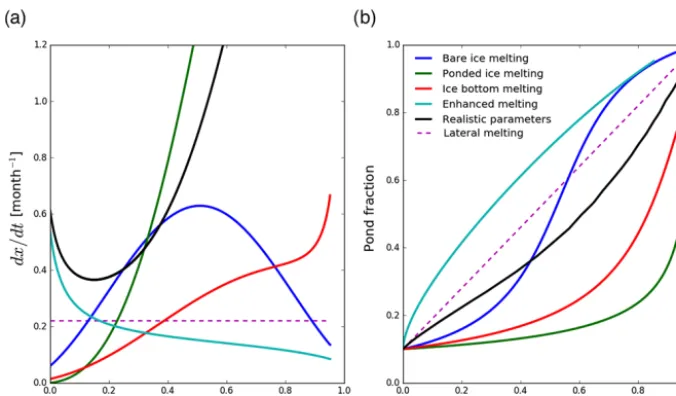
Figure 8. (a)Dependence of growth rate on pond coverage for different modes of pond growth. Theyaxis shows the growth rate, ddxt, for each of the growth modes calculated using the default parameters andxi=0. Pond growth rate for bare ice melting (blue line) first increases up to a certain pond coverage and then decreases. Ponded ice melting (green line) increases with pond coverage fromddxt =0 atx=0 to very high values at high pond coverage. The ice bottom melting rate (red line) gradually increases with pond coverage. The vertical enhanced melting rate (cyan line) decreases with pond coverage. The black line represents a realistic combination of the four growth modes and shows that pond growth is dominated by enhanced melting early in the season and by freeboard sinking late in the season. The dashed magenta line represents lateral melting estimated using parameters described in Sect. 7.1.(b)Solutions to Eq. (26) when only one of the growth modes is active. Thexaxis shows the normalized time, where 0 corresponds to the beginning of the melt and 1 to entire floe being flooded.
Eq. (26) when only one of the strengths is nonzero, assum-ing a first-year ice topography. Figure 9 shows the evolution of pond coverage distribution when only one of the strengths is nonzero.
All modes of growth depend in the same way on the bulk ice density,ρb. Each of the strengths is inversely proportional
to ρb, meaning that ponds grow faster on ice with a lower
bulk density. The effect is, however, modest: within a reason-able range of 916 kg m−3> ρb>750 kg m−3, pond growth
rate can vary by at most 20 %.
We will first discuss freeboard sinking. Common to all modes of freeboard sinking is the dependence on ice thick-ness. Each freeboard sinking growth mode is inversely pro-portional to the ice thickness,Sfs∗∝ 1
H, meaning that, all else equal, ponds grow proportionally slower on thicker ice.
Although ice roughness may have a different effect on each of the individual modes of freeboard sinking, for sim-plicity we will assume that they are all affected by rough-ness in the same way, as parameterized in Eq. (29). In that case, each of these strengths is roughly proportional to the square of the nondimensional ice roughness,Sfs∗ ∝ ˆσ2, mean-ing that pond growth due to freeboard sinkmean-ing is suppressed on smooth ice.
We will now focus on individual components of freeboard sinking. The parameter Sbi∗ controls pond growth by free-board sinking due to melting bare ice. On first-year ice, ow-ing to the shape of the hypsographic curve, the pond growth rate by bare ice melting increases up to a certain pond
cov-erage and decreases afterwards (Fig. 8, blue line).Sbi∗ is pro-portional to the fluxFbiand depends on the initial pond
cov-erage asSbi∗ ∝(1−xi)2. The quadratic dependence on ini-tial bare ice fraction means that ponds on floes with less initial pond coverage grow faster. It also means that floes that start off less ponded can at some point become more ponded than floes that start off more heavily ponded. We can see this in Fig. 9a, where the pond coverage distribu-tion narrows up to a certain point, after which it starts to widen again because floes with lowerxi overtake the floes with higherxi. Using the default values of physical parame-ters ofFbi=85 W m−2,H=1.5 m,xi=0.2, andσˆ =0.55, we getSbi∗ ≈0.13 month−1.
The parameter Smp∗ controls pond growth by freeboard sinking due to melting ponded ice. The pond growth rate increases with pond fraction from 0 atx=0 to very high values at high pond coverage and can be the dominant mode of pond growth if the pond coverage is high enough (Fig. 8, green line). For this reason, giving a representative number to pond growth rate, such asSmp, is only meaningful if the
melt season is short enough such that pond coverage during that period does not change substantially. The dependence on initial pond coverage isSmp∗ ∝xi(1−xi). For this reason the pond coverage distribution widens over time whenSmp∗
is dominant (Fig. 9b). Using Fmp=171 W m−2 and other
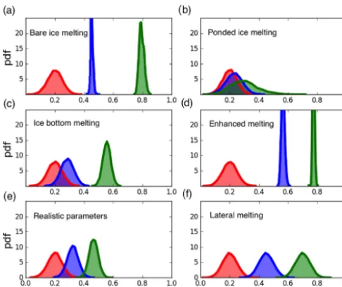
Figure 9.In this figure we have evolved an ensemble of 105floes with varying initial pond coverage according to Eq. (26) when only one of the growth modes is active. Red curves represent the ini-tial pond fraction distribution, blue curves represent the pond frac-tion distribufrac-tion after a time, t, while the green curves represent the pond fraction distribution after 2t. A time used in panel(a)is t= 1
2 1−xi
Sbi , in panel(b)it ist=
1 6
1−xi
Smp , and in panels(c)through(f) it ist= 1
4 1−xi
S , wherexi is the mean pond fraction of the initial distribution andSis an appropriate strength. We show how differ-ent growth modes have differdiffer-ent effects on the pond fraction distri-bution.(a)Bare ice melting first narrows the distribution and then widens it.(b)Ponded ice melting widens the distribution.(c) Bot-tom ice melting narrows the distribution, while the mean of the dis-tribution increases at an increasing rate.(d)Enhanced melting nar-rows the distribution, while the mean of the distribution increases at a decreasing rate.(e)Using realistic parameters, the pond distri-bution slowly narrows and accelerates. (f)Due to lateral melting, pond coverage distribution does not change width, and the growth is linear.
the pond coverage is higher. For example, Smp∗ andSbi∗ are roughly the same atx=0.35, while atx=0.5Smp∗ is roughly twice as large asSbi∗.
The parameter Sbot∗ controls pond growth by freeboard sinking due to melting of the ice bottom. The pond growth rate due to bottom melting increases with increasing melt pond fraction, although more gradually than in the ponded ice melting case (Fig. 8, red line). Since the growth rate is proportional to the bare ice fraction,Sbot∗ ∝(1−xi), the pond coverage distribution gets concentrated over time (Fig. 9c). Using Fbot=20 W m−2 and other parameters the same as
above, we get Sbot∗ ≈0.04 month−1. The contribution from ice bottom melting becomes larger than the contribution from bare ice melting only at highx.
Now, we will turn to enhanced melting. The parameterSem∗
controls pond growth by enhanced melting and is the least constrained in our model due to the many poorly constrained
physical processes that potentially contribute to it. Here we will only consider enhanced melting due to height-dependent processes (Eq. 24) and leave lateral melting for the discus-sion (Sect. 7.1).
Because the growth rate by enhanced melting is inversely proportional to the hypsographic curve, pond growth by en-hanced melting is very fast at the beginning of the melt and decelerates afterwards (Fig. 8, cyan line). The enhanced melting strength is inversely proportional to the square of the ice thickness,S∗em∝ 1
H2, meaning that it is significantly
more sensitive to variations in thickness than freeboard sink-ing. However, it is significantly less sensitive to variations in ice roughness (Eq. 29). Even on perfectly smooth ice,
ˆ
σ=0, ponds will grow due to enhanced melting. In that case, however, lateral melt, rather than height-dependent enhanced melting, may dominate.
The strength of enhanced melting is proportional to the height below which enhanced melting is operational,Sem∗ ∝
1s. If we take ice wetting as a physical example, this means that enhanced melting is sensitive to microphysical processes that determine how high above sea level the ice will be wet. The dependence on the parameter k depends on its mag-nitude. It appears inSem∗ in the term ds k−1
em/dsfs+1. The term
dsem/dsfsis proportional tok−1. Therefore, if dsem/dsfs
1, enhanced melting is proportional to k−1. However, if dsem/dsfs1, enhanced melting becomes independent ofk.
Using default parameters, we find this transition happens at around k≈1.2. In the example of ice wetting, this means that enhanced melting is sensitive to albedo variations near sea level when ice near sea level has a similar albedo to the rest of the floe. However, if the albedo near sea level is sig-nificantly lower than the average, pond growth is insensitive to variations in properties of ice near sea level.
Enhanced melting is proportional to the cube of the bare ice fraction,Sem∗ ∝(1−xi)3, making it very sensitive to vari-ations in initial pond coverage. For this reason, the pond cov-erage distribution gets quickly concentrated (Fig. 9d), and it is possible for initially less ponded floes to overtake initially more ponded floes. If we assume ice wetting is the only phys-ical process responsible for enhanced melting, we can place a rough estimate onSsm∗ . Takingk=1.7,1s=0.06 m, andt=
30 days, we get for default parametersSem∗ ≈0.31 month−1. This suggests that the contribution to mean pond coverage from enhanced melting is slightly larger than the contribu-tion from freeboard sinking after 30 days of melt.
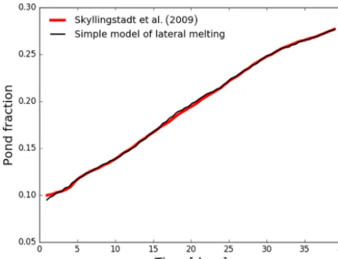
Figure 10.The red curve is the results of Skyllingstad et al. (2009). The black curve is the solution to Eq. (34) withFlat=KlatFmp.
The pond albedo and the shortwave, longwave, sensible, and latent heat fluxes used to findFmpare the same as used in Skyllingstad et
al. (2009) andKlat=1.5. A nearly perfect agreement between the
two curves suggests that a single nondimensional constant,Klat, is
enough to describe pond growth by lateral melting, and the compli-cated physics of lateral melting are important only in determining the value ofKlat.
season and then increases, indicating that freeboard sinking dominates later in the season. The pond coverage distribu-tion using realistic parameters narrows with time (Fig. 9e). Since each growth mode affects the pond coverage distribu-tion in a distinct way, fitting both the evoludistribu-tion of the mean and the standard deviation of the pond coverage distribu-tion in observadistribu-tional data could add constraints on the rel-evant strengths. Using the above values of strengths, we find that after a month of growth bare ice melting contributes to roughly 25 % of mean pond coverage, ponded ice melting contributes to around 13 %, ice bottom melting contributes to around 7 %, and enhanced melting contributes to roughly 55 %.
7 Discussion
7.1 Lateral melting of pond walls by pond water In our model, we focused on vertical changes in topography, and neglected pond growth by lateral melting of pond side-walls by pond water. We will now briefly discuss this possi-bility.
This type of melt was the main focus of Skyllingstad et al. (2009), who carefully calculated the lateral melt rates of pond sidewalls by pond water. The red line in Fig. 10 shows their results. The rate of change of pond fraction due to a
lateral melt fluxFlatis
dxlat
dt = P A
Flat
lρb
, (34)
whereP is the total perimeter of the ponds andAis the area of the floe. IfFlat is constant and the dependence ofP on
pond fraction is weak, pond growth is linear, which explains the roughly linear pond coverage evolution in Skyllingstad et al. (2009). In Fig. 10, black line, we solve Eq. (34) assuming a lateral melt flux proportional to the ponded ice melting flux,
Flat=KlatFmp, where Klat is a constant. We use the same
energy fluxes used by Skyllingstad et al. (2009) and esti-matePA≈0.1 m−1from the aerial photographs taken during SHEBA. A nearly perfect match is obtained withKlat=1.5.
Therefore, a single constant that relates the rate of melt of ponded ice to the rate of melt of pond walls,Klat, is enough
to capture the effects of lateral melting on pond growth. This suggests that the complicated physics of lateral melting can, to a large extent, be ignored. More work would, however, be needed to determine to what degreeKlatvaries under
differ-ent circumstances.
If we ignore the topographic variation above sea level, pond growth due to enhanced melting also becomes linear (Eq. 20). Therefore, lateral melting can approximately be considered a contribution to enhanced melting,Sem, although
it scales differently with physical parameters than the height-dependent enhanced melting (Eq. 24). It is important to note that in this model lateral melt does not depend on ice thick-ness,H, or on initial pond coverage,xi, although, in reality, it may depend on these to some degree. For this reason, the pond coverage distribution width does not change in time, while the mean increases linearly (Fig. 9f).