Interpreting SBUV smoothing errors: an example using the quasi-biennial oscillation

(1)

Atmos. Meas. Tech., 6, 2089–2099, 2013 www.atmos-meas-tech.net/6/2089/2013/ doi:10.5194/amt-6-2089-2013

Sciences

Atmospheric

Chemistry

and Physics

Open Access

Atmospheric

Chemistry

and Physics

Open Access Discussions

Atmospheric

Measurement

Techniques

Open Access

Atmospheric

Measurement

Techniques

Biogeosciences

Open Access Open Access

Biogeosciences

Discussions

Climate

of the Past

Climate

of the Past

Discussions

Earth System

Dynamics

Earth System

Dynamics

Discussions

Geoscientific

Instrumentation

Methods and

Data Systems

Open Access

_{Geoscientific}

Instrumentation

Methods and

Data Systems

Geoscientific

Model Development

Geoscientific

Model Development

Discussions

Hydrology and

Earth System

Sciences

Open Access

Hydrology and

Earth System

Sciences

Ocean Science

Discussions

Solid Earth

Discussions

The Cryosphere

Discussions

Sciences

Discussions

Interpreting SBUV smoothing errors: an example using the

quasi-biennial oscillation

N. A. Kramarova1, P. K. Bhartia2, S. M. Frith1, R. D. McPeters2, and R. S. Stolarski3

1_{Science Systems and Applications Inc., Lanham, MD, USA} 2_{NASA Goddard Space Flight Center, Greenbelt, MD, USA} 3_{John Hopkins University, Baltimore, MD, USA}

Correspondence to: N. A. Kramarova ([email protected])

Received: 31 January 2013 – Published in Atmos. Meas. Tech. Discuss.: 19 March 2013 Revised: 26 July 2013 – Accepted: 30 July 2013 – Published: 22 August 2013

Abstract. The Solar Backscattered Ultraviolet (SBUV)

ob-serving system consists of a series of instruments that have been measuring both total ozone and the ozone profile since 1970. SBUV measures the profile in the upper stratosphere with a resolution that is adequate to resolve most of the im-portant features of that region. In the lower stratosphere the limited vertical resolution of the SBUV system means that there are components of the profile variability that SBUV cannot measure. The smoothing error, as defined in the opti-mal estimation retrieval method, describes the components of the profile variability that the SBUV observing system can-not measure. In this paper we provide a simple visual inter-pretation of the SBUV smoothing error by comparing SBUV ozone anomalies in the lower tropical stratosphere associated with the quasi-biennial oscillation (QBO) to anomalies ob-tained from the Aura Microwave Limb Sounder (MLS). We describe a methodology for estimating the SBUV smooth-ing error for monthly zonal mean (mzm) profiles. We con-struct covariance matrices that describe the statistics of the inter-annual ozone variability using a 6 yr record of Aura MLS and ozonesonde data. We find that the smoothing er-ror is of the order of 1 % between 10 and 1 hPa, increas-ing up to 15–20 % in the troposphere and up to 5 % in the mesosphere. The smoothing error for total ozone columns is small, mostly less than 0.5 %. We demonstrate that by merging the partial ozone columns from several layers in the lower stratosphere/troposphere into one thick layer, we can minimize the smoothing error. We recommend using the fol-lowing layer combinations to reduce the smoothing error to about 1 %: surface to 25 hPa (16 hPa) outside (inside) of the narrow equatorial zone 20◦S–20◦N.

1 Introduction

(2)

of this paper is to demonstrate the benefits and limitations of the SBUV retrieval algorithm and provide clear recommen-dations for SBUV data users.

In Sect. 2 we visually illustrate the SBUV smoothing error due to the limited vertical resolution. We then describe the methodology used to estimate the smoothing error for the SBUV monthly zonal mean (mzm) ozone profiles. We also introduce and analyze parameters that compose the smooth-ing error. In Sect. 3 we analyze the patterns of the SBUV smoothing error and make recommendations for best use of the data. In the last section we summarize our results. Here-after we will use “SBUV” to refer to all instruments.

2 Smoothing error

The primary source of error in the SBUV retrieval algorithm, particularly in the troposphere and lower stratosphere, is the smoothing error due to the limited vertical resolution of the SBUV observing system (Bhartia et al., 2012). The smooth-ing error represents the difference between the retrieved pro-file and the true propro-file due to vertical smoothing by the re-trieval algorithm and a potential bias introduced by a priori constraints (Rodgers, 2000). When the vertical resolution of the observing system is low, the retrieval algorithm relies on the a priori constraints, which could introduce biases into the retrieved profiles. Therefore the smoothing error depends on the vertical resolution of the observing system, the accuracy of the a priori data, and the magnitude and inter-level corre-lations of the natural ozone variability (Rodgers, 2000). For the first time with the v8.6 data set we include estimates of the smoothing error for the mzm SBUV data product, also newly available in v8.6.

2.1 QBO Detection: a smoothing error example

A vivid example of the smoothing error is the misrepre-sentation of the quasi-biennial oscillation (QBO) signal in the SBUV data in the lower tropical stratosphere (e.g., Hol-landsworth et al., 1995). The QBO is a quasi-periodic oscilla-tion between easterly and westerly regimes of the equatorial zonal wind, which in turn effects the distribution of chemical constituents, such as ozone, water vapor, and methane, due to induced circulation changes (e.g., Baldwin et al., 2001). The period of the QBO varies from 24 to 32 months with an average period of about 28 months. One of the pronounced features of the equatorial QBO is its downward vertical prop-agation with a rate of about 1 km per month (e.g., Baldwin et al., 2001).

Figure 1 shows time series of the deseasonalized mzm ozone anomalies obtained from NOAA17 SBUV/2 (black lines) and Aura Microwave Limb Sounder (MLS) (red lines) over the tropics (0–5◦N) for several layers in the strato-sphere. The deseasonalized anomalies are calculated by sub-tracting seasonal cycles from each data set independently to

remove systematical biases between the observing systems. There is a clear QBO signal in both data sets between 100 and 6.4 hPa, but the phases of the QBO signals are shifted. SBUV “sees” the same phase of the QBO at all layers, while MLS shows a vertical downward propagation of the QBO signal over time. Also, the amplitude of the QBO signal derived from MLS is larger compared to that derived from SBUV. Neither data set shows a QBO above 6.4 hPa. The magenta lines in the panels of Fig. 1 show the MLS anomalies con-volved by the SBUV averaging kernels. The concon-volved MLS anomalies agree well with the SBUV anomalies, meaning that the differences in the original profiles are due solely to the differing vertical resolutions. This is particularly ev-ident in layers below 16 hPa. For the layers between 100 and 6.4 hPa, the convolved MLS now shows the same QBO phase lag as the SBUV measurements. The difference between the deseasonalized MLS and SBUV anomalies shows the portion of ozone variability that the SBUV observing system cannot measure, and this quantity can be understood as the SBUV smoothing error.

We will now describe the methodology for estimating the smoothing error and introduce and analyze parameters that compose the smoothing error.

2.2 Mathematical definition of smoothing error

According to Rodgers (2000) smoothing error can be calcu-lated as

Sserr=(A−I)·C·(A−I)T, (1)

where I is a unit matrix, A is a matrix that represents the sensitivity of the SBUV retrievalxˆ to the true statex:A= ∂x/∂xˆ ; and C is the covariance matrix of an ensemble of states about the mean state, calculated as

C=covn(x− ¯x)(x− ¯x)To. (2) In Eq. (2),x is a set of independent high-resolution ozone profiles that characterize the ozone variability.

In this representation, the resulting quantity Sserr is the

smoothing error covariance matrix, which can be understood as an “error pattern” (Rodgers, 1990). Sserris defined by two

parameters: the SBUV A matrix and the covariance matrix

C. In short, the A matrix shows how information from

(3)

Fig. 1. Deseasonalized time series of the ozone mzm columns in the lower tropical stratosphere (0–5◦N). Black lines correspond to SBUV anomalies, red lines show MLS anomalies and magenta lines indicate convolved MLS anomalies. The MLS mixing ratio profiles were converted first to the partial ozone columns at the SBUV layers.

2.3 SBUV A matrix

2.3.1 SBUV version 8.6 algorithm

In this section we outline the main features of the SBUV v8.6 retrieval algorithm, fully described by Bhartia et al. (2012), that are relevant to the present study. In v8.6 the optimal es-timation technique (Rodgers, 2000) is used to retrieve ozone profiles as partial ozone columns (DU per layer) at 80 pres-sure layers plus a top layer above 0.1 hPa. The seasonal ozone climatology, derived from Aura MLS and ozonesonde ob-servations (McPeters and Labow, 2012), is used by the re-trieval algorithm as the a priori information. The a priori covariance matrix Sa is constructed assuming that the

vari-ance at each layer is equal to a constant fraction of the a pri-ori, and that adjacent layers are highly correlated: Sa(i,j)=

σ2xa(i)xa(j )e−|i−j|/Nc , wherexa is the SBUV a priori;i

andj are layer indices;σ2is the fractional ozone variance, andNcis a number of adjacent layers that are highly

corre-lated. We setσ=0.5 andNc=12 (∼10 km) in the v8.6

al-gorithm. The algorithm uses the same a priori covariance ma-trix for all latitude bins and seasons. The measurement error covariance matrix Seis constructed as a diagonal matrix with

the diagonal elements σe=0.43 N value, whereN value

is the logarithm of the backscattered radiance to solar ir-radiance ratio: Nvalue= −100 log10I /I0(see Bhartia et al.,

2012).

In v8.6 ozone profiles are reported as partial ozone columns (DU per layer) at 20 pressure layers (plus a top layer above 0.1 hPa) by combining ozone in every 4 retrieved lay-ers. The 81 layers (80 plus a top layer) are needed to increase the accuracy of the forward model calculations, but the ver-tical resolution of the SBUV measurement system is much coarser, thus it is reasonable to report data at thicker layers. All correlative quantities, such as a priori, Jacobian, A ma-trix, etc., are reported at the same 20 layers. The total ozone columns are calculated as sums of the partial ozone columns at all 21 layers.

(4)

2.3.2 SBUV averaging kernels

The SBUV A matrix has dimensions of number of layers by number of layers, though the top layer is not included, so the dimensions are 20 by 20. The A matrix shows how infor-mation from measurements and a priori are utilized during the retrieval process. A column of the A matrix at a given layerl (wherel is a layer index from 1 to 20) gives the re-sponse of the retrieval at each layer to a delta-function pertur-bation of ozone amount in layerl; a row of the A matrix at a given layerlindicates the sensitivity of the retrieved ozone at layerlto delta-function perturbations of ozone at each layer (Rodgers, 2000). Rows of the A matrices are called the av-eraging kernels (AK), while columns are referred to as the response functions. Hereafter, we will follow Rodgers termi-nology and use a term “AK” to refer to rows of the A matrix. The shape of the AK for each layer describes the vertical resolution of the observing system at that layer. An idealized AK for a defined layer would have aδ-function shape with an integrated value of about one, and a width within the bound-ary of the layer. Limitations of the resolution are indicated when the AK peak is very broad and displaced in altitude (Rodgers, 2000).

The A matrix is relevant to profiles of partial ozone columns in units of DU per layer, but the shapes of averaging kernels (rows of A matrix) are different from the well-known bell shape. To simplify visual analysis, we show rows of nor-malized An matrix in Fig. 2. The normalization is done as

follows:

An(i, j )=A(i, j )·xa(j )xa(i), (3)

wherexais the SBUV a priori profile, andiandj are layer

indices from 1 to 20. This normalized An matrix is

appli-cable to the ozone profiles expressed as a fraction from the a priori. We need to emphasize that for the smoothing error calculations the original A matrices have been used.

Figure 2 shows typical normalized SBUV AK for the northern midlatitudes and tropics. The normalized SBUV AK for layers between 16 and 1 hPa have sharp maxima at nominal altitudes. This means that the SBUV algorithm is capable of accurately retrieving layer ozone amounts in this vertical range. The normalized AK for layers below 16 hPa (and above 1 hPa) have broad peaks, which are shifted up-ward (downup-ward) from the layer nominal altitude, showing that the retrievals are more sensitive to ozone changes at higher (lower) layers. In these vertical ranges, the SBUV retrievals contain less information about the true ozone changes at these layers, and the retrieval algorithm relies on the a priori. In the tropics the shapes of the normalized AK for layers below 10 hPa differ from those at midlatitudes (see Fig. 2). Peaks of the normalized tropical AK for layers below 25 hPa are shifted upward with the maximum around 25 hPa, and the amplitudes of the normalized AK are significantly reduced below 60 hPa. Thus, compared to midlatitudes, the tropical retrievals are less sensitive to ozone changes in the

lower stratosphere and troposphere and heavily rely on a pri-ori information.

The number of independent pieces of information avail-able from measurements is given by the diagonal elements of the A matrix, known as degrees of freedom for signal (DFS) (Rodgers, 2000). Note that the diagonal elements of A and

Anare the same. The sum of all diagonal elements of the A

matrix – the total DFS – varies from 3.7 to 6.9 out of the 6–9 wavelengths used in the retrieval algorithm depending on the solar zenith angle (SZA). The retrieval algorithm uses only 6 wavelengths for small SZA and 9 wavelengths for high SZA (Bhartia et al., 2012). As a result the DFS is larger for higher SZA.

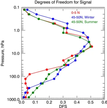
Each diagonal element of the A matrix in turn indicates the DFS for the individual layer. Figure 3 shows the layer DFS for the northern midlatitudes in winter and summer (blue and green lines, respectively) and for the tropics (red line). Peaks of the layer DFS occur between 25 and 1 hPa, where the layer DFS are about 0.5. The total DFS is larger in northern mid-latitudes in winter (5.5) and decreases slightly in summer (5.0). The increase of total DFS in winter is due to the higher SZAs and subsequent increased vertical resolution in the up-per layers. The layer DFS also increases in the upup-per layers above 1 hPa when the satellite approaches the terminator and SZA rapidly increases. In the tropics, SZA does not signif-icantly change with season, and the A matrices are similar for all seasons. The shapes of the layer DFS in the tropics and midlatitudes in summer (red and green lines in Fig. 3) are very similar above 25 hPa, but below 40 hPa the tropical layer DFS abruptly decreases, due to fewer wavelengths used to retrieve ozone at small SZAs and the higher altitude of the ozone peak in the tropics. The longest wavelength used in the retrieval varies from 302 nm at small SZA to 317.5 nm at large SZA to minimize effects of absorbing aerosols.

Since the diagonal elementsds of the A matrix give the DFS per layer, one can estimate the vertical resolution as the number of layers per degree of freedom 1/ds (Rodgers, 2000). The AK show that the vertical resolution of the SBUV algorithm is about 6–7 km near 3 hPa, decreasing to 15 km in the troposphere (Bhartia et al., 2012).

2.4 Ozone mzm covariance matrix

The second parameter that defines the smoothing error is the covariance matrix C, which is used to represent the statistics of ozone variability. We are computing the smoothing error for SBUV mzm profiles, and therefore we need to construct appropriate covariance matrices that characterize the typical year-to-year variability of the ozone mzm profiles for each latitude bin.

(5)

Fig. 2. Typical SBUV averaging kernels for (a) the tropics and (b) northern middle latitudes. Different colors correspond to individual layers, and layer numbers are indicated on the right.

Fig. 3. Typical profiles of layer DFS for the northern midlatitudes in summer (green line), in winter (blue line) and for the tropics (red line). Profiles from NOAA 17, January and July 2007. The connect-ing lines between the data points have no physical meanconnect-ing and are drawn only to guide the eye.

Table 1. We construct MLS mzm time series over the 6 yr pe-riod from January 2005 to December 2010 for each 5◦_zonal bin using version 3.3 daytime-only MLS profiles with SZAs less than 83◦_{. Additional filtering is applied according to} rec-ommendations outlined in the MLS version 3.3 users guide (Livesey et al., 2011). We distribute sonde data by 10◦ lati-tude bins following the guidance provided by McPeters and Labow (2012) to account for limited sampling in some lati-tude bins. The 10◦zonal sonde data for each month and alti-tude level have been interpolated to the 5◦latitude scale. Data from many sonde stations were not available during the Aura

MLS period, so we instead used sonde data over the 6 yr pe-riod from January 2000 to December 2005. The sonde mzm time series were smoothed using a 3 month moving average to reduce noise. Both MLS and sonde profiles were converted into ozone partial columns at SBUV pressure layers.

For each month and latitude bin we merge sonde and Aura MLS mzm profiles in layers 5, 6 and 7 (between 160 and 40 hPa) using a proportional 75, 50 and 25 % weighting for the sonde data in layers 5, 6 and 7. Since the SBUV technique depends on backscattered solar radiation, measurements at high latitudes are not possible in winter months. Thus we estimate the statistics of the ozone variability at high latitudes using data only in months when SBUV ozone measurements exist (see Table 2).

The covariance matrices C for each 5◦ latitude bin have been calculated by employing Eq. (2), and are included in the SBUV mzm data files. The resulting covariance matrix

C for each latitude bin is a matrix with dimensions of

num-ber of layers by numnum-ber of layers (20 by 20; top layer not included), with the diagonal elements equal to the squares of the standard deviations of mzm merged MLS/sonde profiles. The calculated covariance matrices C represent the variabil-ity of the merged MLS/sonde data about their mean. We as-sume that the MLS and sonde measurement error covariance matrices Seare small compared to C, thus the C matrix

rep-resents natural ozone variability. However, we should note that to compute the actual smoothing error we need to know the variability of the “true” ozone profiles about the SBUV a priori. The difference between the estimated and “true” vari-ability will add additional errors in smoothing error calcu-lations, but since the “true” state is not known these errors cannot be estimated.

(6)

Table 1. List of ozonesonde stations used to estimate inter-annual ozone variability for smoothing error calculations over the time pe-riod from 1 January 2000 to 31 December 2005.

Latitude Number of

bin Station Latitude Longitude profiles

80–90◦_S _{South Pole} ₋_89.9 _24.8 ₃₄₇

70–80◦_S _Neumayer ₋_70.7 ₋₈ ₄₂₅

60–70◦S Davis −68.6 79.9 61

Marambio −64.2 −56.7 121

Syowa −69 39.58 397

50–60◦_S _Macquarie ₋_54.5 _158.9 ₂₄₈

40–50◦S Lauder −45 169.6 337

30–40◦_S _Laverton ₋_37.8 _144.7 ₂₅₇

20–30◦S Irene −25.2 28.18 170

Reunion −21 55.48 175

10–20◦_S _Reunion ₋₂₁ _55.48 ₁₇₅

Samoa −14.2 −170 205

Fiji −17.4 178.3 154

0–10◦S Ascension Island −7.58 −14.2 259

Java −7.5 112.6 191

Nairobi −1.27 36.8 343

Natal −5.42 −35.3 241

San Cristobal −0.92 −89.6 216

0–10◦_N _Cotonou _6.21 _2.23 ₃₉

Kuala Lumpur 2.73 101.7 148

Paramaribo 5.81 −55.2 261

Trivandrum 8.29 76.95 45

10–20◦_N _Hilo _19.72 ₋₁₅₅ ₃₁₃

Poona 18.53 73.85 25

20–30◦_N _Hanoi _21.02 _105.8 ₂₃

Hilo 19.72 −155 313

Kagoshima 31.55 130.5 246

Naha 26.2 127.6 245

30–40◦N Boulder 40.02 −105 291

Huntsville 34.72 −86.6 228

Madrid 40.46 −3.65 152

Tateno 36.05 140.1 333

Wallops 37.93 −75.4 241

40–50◦_N _{Canada (Yarmouth, Kelowna)} ₄₇ ₋₉₂ ₁₃₈

Hohenpeisenberg 47.8 11.02 755

Payerne 46.8 6.95 904

Sapporo 43.05 141.3 275

50–60◦_N _Edmonton _53.55 ₋₁₁₄ ₂₆₉

Goose 53.32 −60.3 266

Lindenberg 52.21 14.12 288

Uccle 50.8 4.35 823

60–70◦_N _Churchill _58.75 ₋₉₄ ₂₂₁

Lerwick 60.13 −1.18 233

Sodankyl¨a 67.39 26.65 409

70–80◦N Ny- ˚Alesund 78.93 11.88 521

Resolute 74.72 −94.9 148

Scoresbysund 70.49 −21.9 188

Thule 76.53 −68.7 66

80–90◦_N _Alert _82.5 ₋_62.3 ₃₀₀

a percent of the mean annual SBUV a priori at each latitude (also see Fig. S1 in Supplement, which shows profiles for all latitude bins). Standard deviations vary between 2 and 15 %, increasing in the troposphere and lower stratosphere. However, in the tropical lower stratosphere between 100 and

Fig. 4. Vertical profiles of the square roots of diagonal elements of the covariance matrix for three latitude bins as percent relative to the a priori. These quantities are equal to the standard deviations of the mzm profiles.

10 hPa standard deviations are larger compared to mid and high latitudes due to the QBO.

Off-diagonal elements of C reveal correlations among the layers. Figure S2 in the Supplement shows correlation pat-terns of C for four different latitude bins. If the correla-tion between any two layers is high, the corresponding off-diagonal elements will also be large, and vice versa. We do not analyze off-diagonal elements of C here, because a sim-ple sensitivity test in which the smoothing error was calcu-lated with the off-diagonal elements of covariance matrices set to zero showed that in our case the off-diagonal elements had a very small effect on the smoothing error values. For this reason, the mismatch of the time periods between MLS (2005–2010) and sonde measurements (2000–2005) used to construct the covariance matrices C should not affect the smoothing error calculations, because only the off-diagonal elements of C, which indicate the inter-level correlation, are sensitive to the time mismatch. We expect the ozone vari-ances (presented by the diagonal elements of C) over the two considered 6 yr time periods to be very similar. Nevertheless off-diagonal elements of the covariance matrices C are in-cluded in the computation of the smoothing error.

3 Application of smoothing error concept to SBUV data analysis

For each SBUV mzm profile the smoothing error covariance matrix Sserrwas calculated using Eq. (1). All elements

(diag-onal and off-diag(diag-onal) of the C and A matrices are included in the computation of the smoothing error. The diagonal el-ements of Sserrrepresent the error variances of the elements

(7)

missed

month 6 4 3 2 1 3 4 5

of Sserr indicate the inter-level error correlations (Rodgers,

1990). When the off-diagonal elements of Sserrindicate that

the errors are highly correlated, then we have more informa-tion aboutx (Rodgers, 1990) and the errors are expected to be smaller.

It is not easy to analyze and interpret errors represented in terms of the smoothing error covariance matrix Sserr(see

Fig. S3 in Supplement). To simplify the analysis, we ignore inter-level correlation and assume that the square roots of the diagonal elements of Sserrrepresent the smoothing errors for

individual layers. We also calculated eigenvectors of Sserrand

found that in our case diagonal elements provide a reason-able estimation of the layer smoothing errors. Figure S4 in the Supplement shows the five first eigenvectors of Sserr. The

smoothing error for total ozone is calculated as a square root of the sum of all elements of Sserr (including off-diagonal

elements). In the mzm SBUV files we report the smoothing error as a percent of the retrieved layer ozone amount.

3.1 Profile and total ozone smoothing error

Figure 5 shows profiles of the smoothing error at 45–50◦N in winter and summer (blue and green lines, respectively) and at 0–5◦N (red line). Figures S5–S7 in the Supplement also demonstrate profiles of the smoothing errors for differ-ent seasons and latitude bins. In the stratosphere between 10 and 1 hPa, where the SBUV vertical resolution is the high-est, the smoothing errors are of the order of 1–2 %. Larger smoothing errors (in some cases as large as 15–20 %) oc-cur in the troposphere. Errors also increase up to 5 % in the mesosphere above 1 hPa.

In the midlatitudes the layer smoothing errors vary with season due to seasonal changes of the AK. It is important to remember that the covariance matrix is a function of latitude only. Thus, all temporal changes in the smoothing errors are caused by the temporal changes in the AK. Overall, there is a very good consistency between seasonal changes of the layer DFS and smoothing error (Figs. 3 and 5). At those layers where the DFS is larger the corresponding smoothing errors are smaller and vice versa.

Fig. 5. Typical profiles of SBUV smoothing error (% from the mean a priori profile) for the northern midlatitudes in summer (green line), in winter (blue line) and for the tropics (red line). Profiles from NOAA 17, January and July 2007.

In the tropical stratosphere below 10 hPa, the layer smoothing errors are notably greater compared to the mid and high latitudes. We previously noted a decrease of the tropical layer DFS below 40 hPa. However, the smoothing error increases in the tropics primarily because of the larger inter-annual ozone variability in the tropical lower strato-sphere associated with the QBO (see Fig. 4). In very few cases, for example in layers 6 (100–63 hPa) and 10 (16– 10 hPa) in the tropics, 10◦S–10◦N, the smoothing errors are larger than the estimated ozone standard deviations (square roots of the diagonal elements of C, Fig. 4). This is a limita-tion of our approach considering only the diagonal elements of Sserrand ignoring inter-level error correlations to estimate

the layer smoothing errors.

Figure 6 shows time series of the total ozone smoothing error at 0–5◦N and 45–50◦N. The total ozone smoothing er-ror is calculated as a square root of the sum of all elements of Sserr. Smoothing errors for the total ozone vary between

(8)

a significant role in defining the error range for total ozone. The total ozone errors notably increase when the satellites approach the terminator and SZA increases. This might seem contradictory, since the total DFS increases with increasing SZA due to the larger number of wavelengths used to retrieve ozone at high SZA, implying that we have more information from measurements. But the increase in total DFS is related to increased sensitivity in the upper layers, not in the lower layers, which dominate total ozone. In the lower layers the diagonal elements of A change little with the SZA, while the off-diagonal elements of A in turn are very sensitive to SZA changes and decrease as SZA increases. Thus, as a result the total ozone smoothing error increases with increasing SZA.

We confirmed these results by running a sensitivity test in which the smoothing error was calculated with the off-diagonal elements of A set to zero. The changes to the layer smoothing error were small, but the total ozone smoothing errors increased by a factor of 5–10 (up to 2–6 %) when off-diagonal elements of A were ignored.

3.2 Recommendations for reducing the smoothing error

As we demonstrated, the smoothing error in the lower strato-sphere and tropostrato-sphere can be significant and caution should be taken when comparing SBUV ozone profiles with highly resolved profiles. One approach to such comparisons is to convolve the highly resolved profile with the SBUV AK as shown in Fig. 1. The profile with finer vertical resolution should be degraded first onto the SBUV vertical scale and then convolved using the SBUV A matrix (Rodgers and Con-nor, 2003):

xsmoothed=xa+A·(xhr−xa), (4)

wherexhr is the highly resolved profile converted to partial

ozone columns and degraded to the SBUV vertical scale. However, it is not clear how to convolve a highly resolved profile that covers only a part of the atmosphere. For exam-ple, lidar instruments typically measure ozone only between 20 and 50 km, while the SBUV A matrix is supposed to be applied to the entire profile from the surface to top of the at-mosphere. Liu et al. (2010) use MLS partial ozone columns complemented with Ozone Monitoring Instrument (OMI) re-trievals below 215 hPa to convolve MLS ozone profiles with OMI AK. But different observing systems have different sen-sitivities and vertical resolutions, and this approach might “project” the uncertainties of one observing system onto the other. Alternatively, the missing part of the profile could be assumed to be equal to the a priori, and then the term in brackets in Eq. (4) will be equal to zero in the vertical range where measurements are missing.

We tested these two approaches to convolving Aura MLS profiles (which cover the vertical range between 250 and 0.1 hPa) with the SBUV A matrix. In the first approach we extended MLS profiles below 250 hPa with SBUV retrievals,

Fig. 6. Time series of the SBUV smoothing error for mzm total ozone column. (a) for 40–45◦N latitude zone and (b) for 0–5◦N latitude zone. Different colors correspond to individual SBUV in-struments.

and in the second approach we used the SBUV a priori pro-files. We found that the difference between the two convolved profiles is fairly small (less 0.5 %) in the vertical range be-tween 25 and 1 hPa, where the SBUV vertical resolution is the highest. At the same time, between 250 and 25 hPa, where the SBUV vertical resolution is limited, the difference between the two approaches was up to±3 %. We found even larger differences (up to±10 %) between the two approaches when we convolved lidar profiles. These differences reflect an additional source of uncertainty in the convolved profile.

To avoid these complications, we propose merging sev-eral layers in the lower stratosphere/troposphere, where the smoothing errors are large, into a single thick combined layer. If the thickness of the combined layer is close to the vertical resolution of the measured signal, then the smooth-ing error for the combined layer will decrease. The DFS of the combined layer is equal to the sum of the “parent” layer DFS. The analysis of the AK (see Fig. 2) indicates a limita-tion of the retrievals below 25 hPa (below 16 hPa) outside the tropics (in the tropics). Thus we test the resulting smoothing error when combining all layers below these thresholds.

(9)

Figure 7 shows the smoothing error as a function of lat-itude for several layer combinations. It is very important to note that even when the smoothing error for any indi-vidual layer in the troposphere/lower stratosphere is large, the smoothing error for the combined layer is substantially less. The high negative inter-level correlation of errors (off-diagonal elements of Sserr)plays a significant role in

reduc-ing the merged layer error (see Supplement Fig. S3). The smoothing errors are larger in the tropics compared to the mid and high latitudes. At high latitudes errors are larger in winter and smaller in boreal summer as the SZA changes.

In the narrow tropical zone between 20◦S and 20◦N, the smoothing errors are about 2–3 % for the surface–25 hPa and 250–25 hPa layers (see Fig. 7a, c). The smoothing error drops to about 1 % in the tropics when all layers up to 16 hPa are combined (see Fig. 7b, d). If we require the smoothing er-ror for the combined layer to be∼1 % or less (1σ interval), this condition is satisfied for the layer combinations from the surface (or from 250 hPa) to 25 hPa outside of the tropics. In the narrow tropical zone between 20◦S and 20◦N the upper boundary for the combined layers should be extended up to 16 hPa. With caution, users might choose other layer combi-nations depending on the scientific objectives of the study.

Comparisons with independent measurements in the de-fined broad layers support the theoretical results presented above. Comparisons of SBUV ozone amounts in the lower stratosphere/troposphere layer with Aura MLS (Kramarova et al., 2013) showed that the standard deviations of the dif-ferences between SBUV and MLS mzm measurements in the tropics decreased from 3–4 % for the 250–25 hPa layer to 1 % for the 250–16 hPa layer. Labow et al. (2013) show a±5 % agreement between ozone amounts in the surface– 25 hPa layer measured by the SBUV and several ozonesonde stations over a 40 yr time period.

3.3 QBO detection: interpretation of the SBUV smoothing error

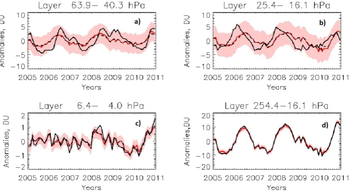
In this section we will discuss a simple interpretation of the SBUV smoothing error by considering again the QBO ozone anomalies in the lower tropical stratosphere. Figure 8 shows the time series of the mzm seasonal anomalies for three in-dividual layers and the combined layer (250–16 hPa) in the equatorial stratosphere. Red lines show the SBUV anomalies and black lines represent Aura MLS anomalies. The shad-owed pink areas indicate the ±2σ range of the calculated

Fig. 7. Smoothing error as a function of latitude for different combi-nations of layers in the lower stratosphere/troposphere: (a) surface– 25 hPa; (b) surface–16 hPa; (c) 250–25 hPa; and (d) 250–16 hPa. Blue lines show errors in winter months (DJF) and red lines errors in summer months (JJA).

SBUV layer smoothing error. At each layer in the lower stratosphere the amplitudes of the ozone anomalies asso-ciated with the QBO are of the same order as the SBUV smoothing errors. Thus, the smoothing error can be under-stood as the limit (or range) of the SBUV sensitivity – if the amplitude of ozone anomalies at a particular layer is less than the corresponding layer smoothing error, the observing sys-tem cannot retrieve these anomalies. It is also important to note that the differences between MLS and SBUV anoma-lies are within the 2σ smoothing error bars. This means the instruments are measuring the same ozone profile and the difference between the two retrieval results is indeed due to the SBUV smoothing error. However, when we merge the recommended layers, the SBUV integrated ozone column contains the QBO signal with a proper amplitude and phase (Fig. 8d), and the smoothing error is substantially less than the amplitude of the QBO.

(10)

Fig. 8. Time series of the deseasonalized ozone anomalies obtained from SBUV and Aura MLS for several layers in the tropical stratosphere: (a) 63–40 hPa layer; (b) 25–16 hPa layer; (c) 6–4 hPa layer; and (d) 254–16 hPa layer. Red lines show SBUV anomalies along with the corresponding smoothing errors (shadowed pink areas indicate±2σ range). Black lines show MLS anomalies, and black dashed lines indicate convolved MLS anomalies. The 254–16 hPa ozone columns (for both SBUV and MLS) were calculated by simply summing partial ozone columns in six individual layers (layers 4–9).

4 Conclusions

In this study we present the methodology used to estimate the smoothing error for SBUV ozone monthly zonal mean pro-files. The smoothing error represents the error in the vertical profile due to the limited vertical resolution of the observ-ing system. The smoothobserv-ing error depends on two parameters – the SBUV averaging kernels that characterize the retrieval algorithm and its vertical resolution, and the covariance ma-trix that describes the natural variability of ozone fields. To estimate the smoothing error for the monthly zonal mean profiles, we constructed covariance matrices that character-ize the inter-annual ozone variability for each latitude bin by using Aura MLS and sonde monthly zonal mean profiles over a 6 yr time period.

Between the 10 and 1 hPa layers the smoothing error is about 1 %. Outside of this vertical range the smoothing er-rors increase to as high as 15–20 % in the troposphere. The smoothing errors for total ozone are much smaller, mostly less than 0.5 %. The smoothing errors for the SBUV monthly mean time series over any particular location (for example, overpasses over ground-based stations) can be considered to be the same order of magnitude as the monthly zonal mean errors for the corresponding latitude bin.

The smoothing effect should be taken into account when analyzing SBUV ozone data at individual layers. When sev-eral ozone layers are merged together in the lower strato-sphere and tropostrato-sphere, the corresponding smoothing error decreases. We recommend using the following layer com-binations to reduce the smoothing error to 1 % or less: surface–25 hPa or 250–25 hPa everywhere outside of the

narrow tropical zone from 20◦S to 20◦N. In these tropical latitudes we recommend merging all layers up to 16 hPa.

We found that the amplitude of the QBO ozone anomalies at any individual layer in the lower tropical stratosphere are of the same order as the SBUV layer smoothing error, mean-ing that the observmean-ing system cannot properly retrieve the signal at individual layers. The smoothing error can be un-derstood as the limit (or range) of the SBUV sensitivity. If the amplitude of ozone anomalies at a particular layer is less than the corresponding layer smoothing error, the observing sys-tem cannot properly retrieve these anomalies. This explains why the SBUV algorithm produces an incorrect phase and amplitude of the QBO ozone anomalies at any individual layer and misses the vertical downward propagation of the QBO signal. However, we showed that the SBUV accurately captures both the amplitude and phase of the QBO signal in the thick 250–16 hPa layer.

(11)

satellite ozone data set. We would like to thank two anonymous referees for their thoughtful comments that helped us to improve the manuscript.

Edited by: J. Urban

References

Baldwin, M. P., Gray, L. J., Dunkerton, T. J., Hamilton, K., Haynes, P. H., Randel, W. J., Holton, J. R., Alexander, M. J., Hirota, I., Horinouchi, T., Jones, D. B. A., Kinnersley, J. S., Marquardt, C., Sato, K., and Takahashi, M.: The Quasi-Biennial Oscillation, Rev. Geophys., 39, 179–229, doi:10.1029/1999RG000073, 2001. Bhartia, P. K., McPeters, R. D., Flynn, L. E., Taylor, S., Kramrova, N. A., Frith, S., Fisher, B., and DeLand, M.: Solar Backscatter UV (SBUV) total ozone and profile algorithm, Atmos. Meas. Tech. Discuss., 5, 5913–5951, doi:10.5194/amtd-5-5913-2012, 2012.

DeLand, M. T., Taylor, S. L., Huang, L. K., and Fisher, B. L.: Calibration of the SBUV version 8.6 ozone data product, At-mos. Meas. Tech., 5, 2951–2967, doi:10.5194/amt-5-2951-2012, 2012.

Froidevaux, L., Jiang, Y. B., Lambert, A., Livesey, N. J., Read, W. G., Waters, J. W., Browell, E. V., Hair, J. W., Avery, M. A., McGee, T. J., Twigg, L. W., Sumnicht, G. K., Jucks, K. W., Mar-gitan, J. J., Sen, B., Stachnik, R. A., Toon, G. C., Bernath, P. F., Boone, C. D., Walker, K. A., Filipiak, M. J., Harwood, R. S., Fuller, R. A., Manney, G. L., Schwartz, M. J., Daffer, W. H., Drouin, B. J., Cofield, R. E., Cuddy, D. T., Jarnot, R. F., Knosp, B. W., Perun, V. S., Snyder, W. V., Stek, P. C., Thurstans, R. P., and Wagner, P. A.: Validation of Aura Microwave Limb Sounder stratospheric ozone measurements, J. Geophys. Res. 113, D15S20, doi:10.1029/2007JD008771, 2008.

Ozone with Data from the Dobson/Brewer Network, J. Geophys. Res. Atmos., 118, 7370–7378, doi:10.1002/jgrd.50503, 2013. Liu, X., Bhartia, P. K., Chance, K., Froidevaux, L., Spurr, R. J.

D., and Kurosu, T. P.: Validation of Ozone Monitoring Instru-ment (OMI) ozone profiles and stratospheric ozone columns with Microwave Limb Sounder (MLS) measurements, Atmos. Chem. Phys., 10, 2539–2549, doi:10.5194/acp-10-2539-2010, 2010. Livesey, N. J., Read, W. G., Froidevaux, L., Lambert, A., Manney,

G. L., Pumphrey, H. C., Santee, M. L., Schwartz, M. J., Wang, S., Cofeld, R. E., Cuddy, D. T., Fuller, R. A, Jarnot, R. F., Jiang, J. H., Knosp, B. W., Stek, P. C., Wagner, P. A., and Wu, D. L.: Earth Observing System (EOS) Aura Microwave Limb Sounder (MLS) Version 3.3 Level 2 data quality and description document, Tech. Rep. NASA JPL D-33509, NASA Jet Propul. Lab., Pasadena, California, available at: http://mls.jpl.nasa.gov, 162 pp., 2011. McPeters, R. D. and Labow, G. J.: Climatology 2011: An

MLS and sonde derived ozone climatology for satel-lite retrieval algorithms, J. Geophys. Res., 117, D10303, doi:10.1029/2011JD017006, 2012.

McPeters, R. D., Bhartia, P. K., Haffner, D., Labow, G. J., and Flynn, L.: The v8.6 SBUV Ozone Data Record: An Overview, J. Geophys. Res. Atmos., 118, 8032–8039, doi:10.1002/jgrd.50597, 2013.

Rodgers, C. D.: Characterization and error analysis of profiles re-trieved from remote sounding measurements, J. Geophys. Res., 95, 5587–5595, doi:10.1029/JD095iD05p05587, 1990.

Rodgers, C. D.: Inverse methods for atmospheric sounding, The-ory and Practice; Series on Atmospheric, Oceanic and Planetary Physics, Vol. 2, World Scientific, 2000.