Lithosphere and upper-mantle structure of the southern Baltic Sea estimated from modelling relative sea-level data with glacial isostatic adjustment

(1)

www.solid-earth.net/5/447/2014/ doi:10.5194/se-5-447-2014

Lithosphere and upper-mantle structure of the southern Baltic Sea

estimated from modelling relative sea-level data with glacial isostatic

adjustment

H. Steffen1, G. Kaufmann2, and R. Lampe3

1_{Lantmäteriet, Lantmäterigatan 2c, 80182 Gävle, Sweden}

2_{Freie Universität Berlin, Institut für Geologische Wissenschaften, Fachrichtung Geophysik, Malteserstr. 74–100, Haus D,}

12249 Berlin, Germany

3_{Ernst-Moritz-Arndt-Universität Greifswald, Institut für Geographie und Geologie, F.-L.-Jahn-Str. 16, 17487 Greifswald,}

Germany

Correspondence to: H. Steffen (holger-soren.steffen@lm.se)

Received: 26 November 2013 – Published in Solid Earth Discuss.: 23 December 2013 Revised: 4 April 2014 – Accepted: 4 April 2014 – Published: 10 June 2014

Abstract. During the last glacial maximum, a large ice sheet covered Scandinavia, which depressed the earth’s surface by several 100 m. In northern central Europe, mass redistribu-tion in the upper mantle led to the development of a periph-eral bulge. It has been subsiding since the begin of deglacia-tion due to the viscoelastic behaviour of the mantle.

We analyse relative sea-level (RSL) data of southern Swe-den, Denmark, Germany, Poland and Lithuania to deter-mine the lithospheric thickness and radial mantle viscosity structure for distinct regional RSL subsets. We load a 1-D Maxwell-viscoelastic earth model with a global ice-load his-tory model of the last glaciation. We test two commonly used ice histories, RSES from the Australian National University and ICE-5G from the University of Toronto.

Our results indicate that the lithospheric thickness varies, depending on the ice model used, between 60 and 160 km. The lowest values are found in the Oslo Graben area and the western German Baltic Sea coast. In between, thickness in-creases by at least 30 km tracing the Ringkøbing-Fyn High. In Poland and Lithuania, lithospheric thickness reaches up to 160 km. However, the latter values are not well constrained as the confidence regions are large. Upper-mantle viscosity is found to bracket [2–7]×1020Pa s when using ICE-5G. Employing RSES much higher values of 2×1021Pa s are obtained for the southern Baltic Sea. Further investigations should evaluate whether this ice-model version and/or the

RSL data need revision. We confirm that the lower-mantle viscosity in Fennoscandia can only be poorly resolved.

The lithospheric structure inferred from RSES partly sup-ports structural features of regional and global lithosphere models based on thermal or seismological data. While there is agreement in eastern Europe and southwest Sweden, the structure in an area from south of Norway to northern Ger-many shows large discrepancies for two of the tested litho-sphere models. The lithospheric thickness as determined with ICE-5G does not agree with the lithosphere models. Hence, more investigations have to be undertaken to suf-ficiently determine structures such as the Ringkøbing-Fyn High as seen with seismics with the help of glacial isostatic adjustment modelling.

1 Introduction

During the last colder climatic phase with average surface temperatures being about 10◦_{C lower than today (Petit et}

(2)

area. This narrow band of 100–200 km width was uplifted up to a few tens of metres (Steffen and Wu, 2011). During and after the deglaciation phase, the mass redistribution is reversed, forcing uplift of the formerly glaciated areas and subsidence of the peripheral bulge. These changes are, due to the viscoelastic and thus time-delayed behaviour of the mantle, still observable today.

This dynamic response of the earth during glacial cycles is known as glacial isostatic adjustment (GIA). There are sev-eral observation methods for this process, and Fennoscandia has turned out to be the key area for GIA studies (e.g. Stef-fen and Wu, 2011, and references therein). Relative sea-level (RSL) data provide the longest observational data set from all observations, occasionally dating back several thousands of years. They document the movement of coastlines as a consequence of both the water redistribution between oceans and ice sheets and the deformation of the earth’s surface that occurred in the past.

RSL data can be employed for the determination of the earth’s internal structure, in particular the lithospheric thick-ness and mantle viscosities (e.g. Steffen and Wu, 2011, and references therein). Often, this is done in formerly glaciated areas, e.g. Fennoscandia, the Barents Sea or the British Isles. As an example, Steffen and Kaufmann (2005) subdivided the Fennoscandian RSL data set into RSL data located in the cen-tre around the Baltic Sea and coastal data mainly along the Norwegian coast. They found clear differences in the earth’s structure of the two regions. Vink et al. (2007) subdivided a RSL data set of the southern North Sea into three dis-tinct regional subsets. A regional variation of the lithospheric thickness as well as regionally differing isostatic subsidence curves were determined.

The earth structure beneath northern Europe derived from GIA data can be summarized as follows: in Fennoscandia, the lithosphere is laterally varying with a thick root of more than 200 km in central-east Fennoscandia, becoming thinner towards the west (Steffen and Wu, 2011). Southwest Sweden is predicted to have a lithospheric thickness of about 100 km, and the German North Sea coast as well as the Norwegian Atlantic coast of about 80 km (Vink et al., 2007; Steffen and Wu, 2011). Note that we use the term lithosphere to refer to the strong outer shell of the earth composed of the crust and upper part of the mantle, which both have a purely elastic rheology on the GIA timescale.

Below the lithosphere, investigations have found upper-mantle viscosity to be between 1020 and 1021Pa s (Stef-fen and Wu, 2011). The latest results calculated from dif-ferent data are in the range [3–8]×1020Pa s. The viscos-ity increases towards the lower mantle (Steffen and Kauf-mann, 2005). The lower-mantle viscosity is assumed to be around 1–2 orders of magnitude higher. Its determination, however, is complicated, as the resolving power of all data in Fennoscandia is too low to resolve more accurate values for the lower mantle (Steffen and Wu, 2011).

The values above have mainly been determined with spherically symmetric models using Maxwell rheology. However, other rheologies such as composite rheology (van der Wal et al., 2013) or models with laterally varying litho-spheric thickness and/or mantle viscosities (Wu et al., 2005; Steffen et al., 2006; Wang et al., 2008; van der Wal et al., 2013; Wu et al., 2013) can also fit the observations in Fennoscandia reasonably well.

The lithosphere determined in GIA studies should be com-parable to results from other studies, e.g. seismological stud-ies. However, there are different geophysical definitions of the lithosphere depending on the method used for its determi-nation. There are rheological, petrological, elastic, thermal, electrical and seismic definitions. It is beyond the scope of this paper to discuss individual definitions or their determi-nation in detail, or the relation of one lithosphere definition to another. We therefore refer the interested reader to Tesauro et al. (2009), Eaton et al. (2009) and Artemieva (2009) for a detailed overview. But it has been noted that some of the defi-nitions should coincide, such as the thermal definition and the seismological one (Tesauro et al., 2009). Eaton et al. (2009) define the lithosphere as “a rheological term referring to the strong outer shell of the earth composed of the crust and up-per part of the mantle; also called a mechanical boundary layer”. The seismological lithosphere is generally the high-velocity outer layer of the earth, approximately coincident with the lithosphere as a rheological term, which typically overlies a low-velocity zone (Eaton et al., 2009). The thermal lithosphere is defined by a depth to a constant isotherm or by the depth of the intersection of a continental geotherm either with a mantle adiabat or with a temperature close to mantle solidus (Artemieva, 2009). We will see that the lithospheric structure in northern Europe as derived with GIA modelling and outlined above, partly agrees with thermal and seismo-logical studies on the lithosphere on a broad scale, but only in terms of lateral variation and not in an exact match of thick-nesses.

(3)

exercise, we compare the lithospheric thickness as derived in regional subsets to three lithospheric thickness models avail-able to us.

In Sect. 2, we describe the RSL data used. This is followed by an overview of the modelling technique and the ice mod-els implemented in this study (Sect. 3). Results are presented in Sect. 4 and discussed in Sect. 5. This includes a compar-ison to lithosphere models available to us. Finally, we sum-marize our main findings in Sect. 6.

2 Relative sea-level data

In the past decades mostly basal peat layers (sensu Lange and Menke, 1967) found in sediment cores were used to re-construct the postglacial sea-level rise along the southern and western Baltic coast. However, these sea-level indicators, of-ten scattered over larger areas, may have experienced differ-ent vertical movemdiffer-ents due to isostasy and/or compaction and thus are compromised by large uncertainties in many respects. More recently, new sampling, positioning and dat-ing techniques have allowed the detection of archaeological underwater finds such as settlement refuse, boats, fish weirs and fire places, or drowned in situ tree stumps (Tauber, 2007; Lübke et al., 2011). Such finds provide numerous samples for a distinct site and a specific elevation relative to modern sea level. Other approaches use a set of isolation basins or coastal mires to trace the sea-level variation over a longer period in a very limited area (Yu et al., 2004; Lampe et al., 2011). Such investigations allow the construction of sea-level curves ow-ing to better resolution and minor altitude errors and thus higher precision. They provide an excellent base to test dif-ferent ice-load history models and earth models as well.

For this study we use published data sets from Denmark (Great Belt and Halsskov Fjord: Christensen et al., 1997), northeastern Germany (Schleswig-Holstein: Winn et al., 1986; Jakobsen, 2004; Mecklenburg-Vorpommern: Lampe et al., 2007; Hoffmann et al., 2009; Poland: U´scinowicz, 2003 and a few data from Lithuania: Curonian Lagoon and adja-cent areas: Bitinas et al., 2000, 2002). A common feature of the investigated regions is that the postglacial sea-level rise did not start until the transgressing ocean inundated the Dan-ish Great Belt and invaded the Baltic Basin. Age determina-tions of the earliest marine influence in the southern Baltic therefore lie between 9.4 and 8.0 ka cal BP (Hofmann and Winn, 2000; Rößler et al., 2011; Bennike et al., 2004). Be-cause the maximum depth of the Danish Great Belt amounts to 25 m below sea level, the rising ocean could not invade the Baltic Basin before it inundated this threshold and thus the sea-level change cannot be traced to greater depths. In coastal regions the Pleistocene relief further restricts the depth where the former sea level can be determined.

Therefore, the lowest sea-level indicators used in the study come from offshore areas in the Great Belt and Bay of Kiel, while all other indicators are from near-coastal on- and

off-shore areas that are located at much lesser depths. Mostly, the data used belong to larger data sets compiled by archaeo-logical, palaeoecological or geological investigations. From these sets data were chosen which are evaluated as reliably related to the former sea level, considering the kind of dated material and probability of relocation, sedimentary facies, accuracy of altitude determination and age–depth relations in the entire data set.

In addition to these new data for the southern Baltic Sea coast, we investigate RSL data in the southwestern part of Fennoscandia that were used by Steffen and Kaufmann (2005) and Schmitt et al. (2009). We group these data into five regional subsets according to dominant structures visi-ble in the regional geology (Scheck-Wenderoth et al., 2005) and crust–mantle boundary (Dèzes and Ziegler, 2002), see our additional remarks on each subset below.

The first covers the Oslo Graben and the eastern part of the Norwegian–Danish Basin (Fig. 1). It contains 77 data from northern Denmark (Limfjord) and the Oslo Fjord. Lambeck et al. (1998) used a subset for the Oslo Fjord only while the Limfjord data were included in a Danish subset together with data from the Great Belt. We will see that both regions, Lim-fjord and Oslo Fjord, can be combined into one subset. The second subset includes 44 data from southwest (SW) Swe-den that were used by Lambeck et al. (1998) in a subset for SW Sweden as well. In addition, 12 archaeological data from dated Hensbacka sites around the city of Gothenburg as de-scribed and used in Schmitt et al. (2009) are added result-ing in a total of 56 data for this data set, which is located east of the Teisseyre–Tornquist Zone. The third subset, called Fyn, consists of 128 indicators from the Great Belt and north-eastern Germany, but east of Rostock. These data are located within the Rinkøping-Fyn High and extend the area further east almost parallel to the former ice margin. The fourth sub-set contains 65 data of the bays of Kiel and Lübeck along the western coast of the German Baltic Sea. This area is part of the North German Basin. As there are RSL data which are at the border of the third and fourth subset, we test the influ-ence of these data on the determined best-fitting earth model for each subset. These data are located at Rostock (yellow dots in Fig. 1), Körkwitz (light blue) and the Darss Penin-sula (dark blue). As we test all three locations in each subset, this results in four different subset of “Fyn” and “bays of Kiel and Lübeck”. The fifth subset encompasses 31 indica-tors from Poland and Lithuania. These data are found east of the Teisseyre–Tornquist Zone.

(4)

−50 0 50 100 150 200 250

Land uplift [m

]

0 3 6 9 12 15 18

Time BP [ka]

10˚ 15˚ 20˚

54˚ 54˚

56˚ 56˚

58˚ 58˚

60˚ 60˚

6

5 4 2

3 1

Figure 1. Spatial and temporal distribution of relative sea-level data

used in this study. Colours indicate five regional subsets: (I) South-west Sweden (red), (II) Oslo Graben (dark and light green for Oslo Fjord and Limfjord, respectively), (III) Fyn with Great Belt, Rügen, Usedom (violet), Darss Peninsula (dark blue) and Körkwitz (light blue), (IV) bays of Kiel and Lübeck (orange) and Rostock (yellow), (V) Poland and Lithuania (black). Data uncertainties are indicated by vertical error bars. Geographical information: 1 Oslo Fjord; 2 Great Belt; 3 Fyn; 4 Bay of Lübeck; 5 Darss Peninsula; 6 Rügen. Dashed lines mark the location of the Rinkøping-Fyn High.

of near-field data, here more than 200 m, is much larger than that of the far-field data, which has a range of less than 30 m. The main sea-level change visible in the latter data happens before 7 ka BP. After that, the change is in the metre range.

3 Modelling 3.1 Earth models

The modelling is undertaken with the software package ICEAGE (Kaufmann, 2004), which was successfully used in earlier GIA studies (e.g. Steffen and Kaufmann, 2005; Vink et al., 2007; Steffen et al., 2010). We briefly summarize the

main characteristics and methods only, and refer the reader to Steffen and Kaufmann (2005) for more information.

We employ a spherically symmetric (1-D), compressible, Maxwell-viscoelastic earth model having three layers to be varied; lithospheric thickness, upper- and lower-mantle vis-cosity. The depth of the boundary between upper and lower mantle is set to 670 km. An inviscid earth’s core is set as lower boundary. The viscosity is kept constant within a layer. Elastic parameters are taken from the Preliminary Refer-ence Earth Model (PREM Dziewonski and Anderson, 1981). Lithospheric thickness is varied between 60 and 160 km, upper-mantle viscosity between 1019 and 4×1021Pa s, and lower-mantle viscosity between 1021 and 1023Pa s. Based on former investigations (e.g. Steffen and Kaufmann, 2005; Vink et al., 2007) these values cover plausible values for three-layer models well.

We follow the pseudo-spectral approach described in Mitrovica et al. (1994) and Mitrovica and Milne (1998) for the calculation of relative sea levels with our models. It is an iterative procedure in the spectral domain with a spherical harmonic expansion up to degree 192, which solves the sea-level equation (Farrell and Clark, 1976) for a rotating earth. Relative sea levels are calculated for 1089 (11×11×9) dif-ferent so-called three-layer earth models which are then com-pared to our regional RSL data sets based on a least-squares misfit

χ=

v u u t

1

n n X

i=1

_o

i−pi(aj) 1oi

2

, (1)

withn the number of observations, oi the observed RSL, pi(aj)the predicted RSL for a specific earth modelaj, and 1oi the error of the observed RSL. The lowest value of χ

relates to the best-fitting earth modelabout of the 1089 pro-vided. In addition, we analyse the model confidence within the observational errors by calculating the confidence param-eter

ψ=

v u u t

1

n n X

i=1

_p

i(ab)−pi(aj) 1oi

2

(2)

of the predicted RSL for the best-fitting earth modelpi(ab) to all other earth models. We show the 1σ and 2σuncertainty for models that obeyψ≤1 and 1< ψ≤2, respectively, of the best-fitting earth model.

3.2 Ice models

(5)

of the one presented in Lambeck et al. (1998). The other global ice model is the commonly used ICE-5G ice history (Peltier, 2004). Both RSES and ICE-5G belong to the type of ice models which are constrained by solid-earth models. Hence, best-fitting models usually tend to converge to a ra-dial profile of specific lithospheric thickness and several vis-cosity layers as used in the ice-model generation. This is es-pecially the case when the same observational data are used in an investigation. In our case, we test a large set of RSL data that have not been used to generate the respective ice models. This may either imply modifications for the ice model if the best-fitting earth model is different, or may shed a light into lateral lithosphere and mantle viscosity variations if the ice model is assumed to be correct. RSES is associated with a 1-D earth model that has a lithospheric thickness of 65–85 km, an upper-mantle viscosity of 3–4×1020Pa s and a lower-mantle viscosity about one order of magnitude larger than the upper mantle. ICE-5G’s underlying earth model, called VM2, has a lithospheric thickness of 90 km, and then sev-eral viscoelastic layers in the mantle. The average viscosities in the upper and lower mantle are about 6×1020Pa s and 2×1021Pa s, respectively.

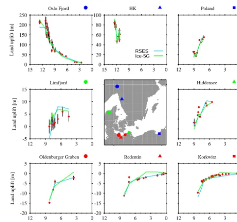
We exemplarily show the extent of the Fennoscandian ice sheet at Last Glacial Maximum of the two models in Fig. 2. There are distinct differences in collapse history, ice height and extent of the models, such as the bridge between Fennoscandia and the British Isles. The ice-sheet maximum is located over the Gulf of Bothnia and central Sweden, with more ice in ICE-5G than RSES. Such differences between the ice models will consequently produce different patterns of rebound in the modelling.

4 Results

We start presentation of the results with a discussion of the best-fitting three-layer earth models (Table 1) for each ice model and regional RSL data set, which includes a brief pre-sentation of results of the different groupings of sea-level data. We calculated the best-fitting earth model for two sub-sets of the Oslo Graben, the Oslo Fjord and Limfjord (see Ta-ble 1). We find almost the same best-fitting earth model for each RSL data subset, and thus combination of Oslo Fjord and Limfjord RSL data is possible. For the grouping of RSL data either in the Fyn or bays of Kiel and Lübeck subset we provide the results of four different combinations. For both ice models, we consider the combination with Rostock data in the bays of Kiel and Lübeck subset as best (Table 1). There is almost no change in the best-fitting earth model pa-rameters for the Fyn subset using RSES, but the misfit gets worse the more data are moved to the other subset. The other subset (bays of Kiel and Lübeck) has the same best-fitting earth model parameters with and without the Rostock data set, but the misfit is better when including the Rostock data. Assigning more easterly located RSL data, of Körkwitz and

Figure 2. Ice extent at Last Glacial Maximum in Fennoscandia from

global ice models (a) RSES (Lambeck et al., 1998) and (b) ICE-5G (Peltier, 2004).

Darss Peninsula, from the Fyn subset to this data set, the earth model parameters change abruptly and the misfit gets worse. Using ICE-5G, there is also a remarkable change in the earth model parameters if RSL data from Körkwitz and Darss Peninsula are moved from one subset to the other. As the misfit gets worse for Fyn when moving more data, and the misfit does not significantly change for the bays of Kiel and Lübeck subset, we use combination (2) in Table 1 in the discussion below.

(6)

Table 1. Best-fitting three-layer 1-D earth models with RSES and ICE-5G ice-load history, respectively, as derived for each regional RSL

data subset. Values in parentheses show theσ1range for each model parameter. If no parentheses appear, theσ1range encompasses the

best-fitting model only.Hllithospheric thickness,ηUMupper-mantle viscosity,ηLMlower-mantle viscosity,χmisfit.

Region Hl ηUM ηLM χ

in km in 1020Pa s in 1022Pa s RSES

SW Sweden 130 (100–160) 4 (3–10) 0.1 (0.1–1) 1.18 Oslo Graben 60 (60–70) 2 4 (0.4–10) 1.58 Oslo Fjord 60 (60–90) 2 4 (0.4–10) 1.61 Limfjord 60 (60–70) 1 (0.5–2) 0.2 (0.2–10) 1.13 Fyn1 90 (70–150) 20 (7–20) 10 (0.7–10) 3.88 Fyn2 90 (70–150) 20 (7–20) 10 (0.7–10) 3.91 Fyn3 90 (70–140) 20 (7–20) 10 (0.7–10) 4.17 Fyn4 100 (80–160) 20 (7–20) 10 (1–10) 4.18 Bays of Kiel and Lübeck1 60 (60–150) 20 2 (2–3) 1.92 Bays of Kiel and Lübeck2 60 (60–150) 20 2 (2–3) 1.84 Bays of Kiel and Lübeck3 110 (60–150) 20 (7–20) 2 (0.3–3) 1.97 Bays of Kiel and Lübeck4 160 (120–160) 20 4 (3–7) 2.01 Polish Baltic Sea 160 (120–160) 20 10 (7–10) 5.70 ICE-5G

SW Sweden 90 (60–140) 2 (0.6–2) 0.1 (0.1–10) 0.87 Oslo Graben 60 (60–70) 2 0.4 (0.3–0.9) 2.19 Oslo Fjord 70 (60–100) 2 1 (0.4–10) 1.44 Limfjord 60 (60–80) 0.7 (0.3–1) 0.1 (0.1–0.2) 1.82 Fyn1 100 (90–110) 2 0.1 3.19 Fyn2 100 (90–110) 2 0.1 3.25 Fyn3 80 (70–90) 4 (4–5) 7 (4–10) 3.47 Fyn4 80 (70–90) 4 (4–5) 7 (7–10) 3.48 Bays of Kiel and Lübeck1 60 (60–120) 7 (6–10) 0.7 (0.3–1) 1.95 Bays of Kiel and Lübeck2 60 (60–70) 4 4 (2–10) 1.95 Bays of Kiel and Lübeck3 100 (70–140) 2 0.1 1.90 Bays of Kiel and Lübeck4 100 (70–140) 2 0.1 1.91 Polish Baltic Sea 80 7 (6–7) 7 (6–9) 5.04

1_{Initial RSL data subsets of Fyn and Bays of Kiel and Lübeck.}

2_{RSL data from Rostock (yellow dots in Fig. 1) are moved from Fyn}1_{to Bays of Kiel and Lübeck}1_. 3_{RSL data from Rostock and Körkwitz (yellow and light blue dots in Fig. 1) are moved from Fyn}1_{to Bays of} Kiel and Lübeck1_.

4_{RSL data from Rostock, Körkwitz and Darss Peninsula (yellow, light and dark blue dots in Fig. 1) are moved} from Fyn1to Bays of Kiel and Lübeck1.

Pronounced differences exist for the upper-mantle viscos-ity. While for ICE-5G only small variances between [2– 7]×1020Pa s appear for the five investigated regions, the viscosity as determined with RSES varies by one order of magnitude with quite high upper-mantle viscosities of 2×1021Pa s for southern Baltic Sea RSL data. In SW Swe-den and Oslo Graben the viscosity values are comparable to those of ICE-5G. Lower-mantle viscosity also shows a wide range of values; however, it has already been often noted that lower-mantle viscosity cannot be well determined with Fennoscandian RSL data due to their low resolving power to such great depths. Lower-mantle viscosity is generally higher than the upper-mantle viscosity. For SW Sweden, this statement needs to be further evaluated as the lower-mantle

(7)

a) f) 3 4 4 5 5 6 6 7 7 8 9 1019 1020 1021

Upper mantle viscosity (Pa s)

60 70 80 90 100 110 120 130 140 150 160

Lithosphere thickness (km)

A 2 3 3 4 4 5 5 6 6 7 8

1021 1022 1023

Lower mantle viscosity (Pa s)

B Oslo Graben 4 5 5 6 6 7 8 9 1019 1020 1021

60 70 80 90 100 110 120 130 140 150 160

A 3 3 4 4 5 5 5 6 6 7 8 9

1021 1022 1023

B Oslo Graben b) g) 2 2 3 3 4 5 1019 1020 1021

60 70 80 90 100 110 120 130 140 150 160

A 2 2 3 3 4 4 5

1021 1022 1023

B SW Sweden 1 2 2 2 3 3 3 4 4 5 1019 1020 1021

60 70 80 90 100 110 120 130 140 150 160

A 1 2 2 2 3 3 3 4 4 5 5

1021 1022 1023

B SW Sweden c) h) 4 4 6 6 6 6 8 8 8 10 10 12 12 14 14 16 16 18 18 20 20 22

2224 26

1019

1020

1021

60 70 80 90 100 110 120 130 140 150 160

A 6 6 6 8 8 8 10 10 12 12 14 14 16 16 18 20 22

1021 1022 1023

B Fyn without Rostock RSL data

4 4 6 6 6 8 8 8 10 10 10 12 12 12 1019 1020 1021

60 70 80 90 100 110 120 130 140 150 160

A 4 6 6 6 8 8 8 10 10 10 12 12 12 14 14 16 16 18 18 20 20 22 24 26 28

1021 1022 1023

B Fyn without Rostock RSL data

d) i) 2 2 4 4 4 6 6 6 8 8 10 10 12 12 14 14 16 16 1019 1020 1021

60 70 80 90 100 110 120 130 140 150 160

A 4 4 4 4 6 6 6 8 8 10 10 12 12 14 16

1021 1022 1023

B Bays of Kiel and Lubeck, and Rostock RSL data

4 4 4 4 6 6 6 6 8 8 8 10 10 12 12 14 14 16 16 18 18 20 20 22 1019 1020 1021

60 70 80 90 100 110 120 130 140 150 160

A 2 4 4 4 4 6 6 6 8 8 10 10 12 12 14 14 16 18

1021 1022 1023

B Bays of Kiel and Lubeck, and Rostock RSL data

e) j) 6 9 9 12 12 15 15 18 18 21 21 24 24 27 27 30 30 33 33 36 36 39 1019 1020 1021

60 70 80 90 100 110 120 130 140 150 160

A 9 9 12 12 12 15 15 15 18 18 21 21 24 24 27 27 30 30 33 36 39

1021 1022 1023

B Poland and Lithuania

6 6 9 9 9 9 12 12 15 15 18 18 21 21 24 24 27 27 30 30 33 33 36 36 39 39 42 42 45 45 48 48 51 1019 1020 1021

60 70 80 90 100 110 120 130 140 150 160

A 9 9 12 12 15 15 15 18 18 18 21 21 21 24 24 24 27 27 27 30 30 33 33 36 39 42

45

1021 1022 1023

B Poland and Lithuania

Fig. 3. Misfit for ice models RSES (a-e) and ICE-5G (f-j), three-layer earth model and different datasets. (A) is the misfit map as a function

of lithospheric thickness and upper-mantle viscosity for a fixed lower-mantle viscosity according to the best-fitting earth model, see Table 1. (B) is the misfit map as a function of upper and lower-mantle viscosities according to the best-fitting earth model for a fixed lithospheric thickness, see Table 1. (a, f) Misfit map for Oslo Graben RSL data (light and dark green dots in Fig. 1). (b, g) Misfit map for SW-Sweden RSL data (red dots in Fig. 1). (c, h) Misfit map for Fyn without Rostock RSL data (violet, dark and light blue dots in Fig. 1). (d, i) Misfit map for Bays of Kiel and L¨ubeck and Rostock RSL data (orange and yellow dots in Fig. 1). (e, j) Misfit map for Polish & Lithuanian RSL data (black dots in Fig. 1). The best 3-layer earth model is marked with a diamond, the light and dark shadings indicate the confidence regions

ψ≤1and1< ψ≤2, respectively.

Figure 3. Misfit for ice models RSES (a–e) and ICE-5G (f–j), three-layer earth model and different data sets. Panel A: the misfit map as

a function of lithospheric thickness and upper-mantle viscosity for a fixed lower-mantle viscosity according to the best-fitting earth model, see Table 1. Panel B: the misfit map as a function of upper- and lower-mantle viscosities according to the best-fitting earth model for a fixed lithospheric thickness, see Table 1. (a, f) Misfit map for Oslo Graben RSL data (light and dark green dots in Fig. 1). (b, g) Misfit map for SW Sweden RSL data (red dots in Fig. 1). (c, h) Misfit map for Fyn without Rostock RSL data (violet, dark and light blue dots in Fig. 1).

(d, i) Misfit map for bays of Kiel and Lübeck and Rostock RSL data (orange and yellow dots in Fig. 1). (e, j) Misfit map for Polish and

(8)

454 H. Steffen et al.: Lithosphere and upper-mantle structure of the southern Baltic Sea

For Fyn as well as the bays of Kiel and Lübeck the 1σ

ranges for the viscosities become much narrower than for SW Sweden. Only lithospheric thickness as determined with RSES may be varied over almost the whole tested parame-ter range. These two data sets as well as that of SW Sweden show the feature of bifurcation in the misfit maps of litho-spheric thickness vs. upper-mantle viscosity. There are two regions of high misfits, one at about 1021Pa s and thinner lithospheric thicknesses, and another one at about 1020Pa s and lower covering the whole thickness range. This lower bound and the “island” at 1021Pa s seem to force the best-fitting model to adopt upper-mantle viscosity values either of [2–7]×1020Pa s or of 2×1021Pa s and larger. Lithospheric thickness is not strongly bounded for these two areas of low fits. While ICE-5G prefers the lower upper-mantle viscos-ity area, RSES tends to higher viscosities. Although the 1σ

range for the RSES results does not cover the lower upper-mantle viscosity range, new deeper and older RSL data and an updated ice model may help shift the results to similar values as determined with ICE-5G.

Another interesting behaviour is that lower-mantle viscos-ity appears to be, except for SW Sweden, clearly determined. This also holds for the Polish and Lithuanian data. Instead, the island at 1021Pa s for upper-mantle viscosity does not appear and lithospheric thickness is better determined (espe-cially for ICE-5G) than for the other regions.

5 Discussion

In the previous section we derived bounds for lithospheric thickness and upper- and lower-mantle viscosity for the dif-ferent regions. We now take closer look at the fitted RSL data. While the locations Oslo Graben and SW Sweden are mainly near-field data with a large time and height/depth range, the other three regional subsets contain far-field data of younger age and smaller depth ranges, i.e. there is only a window of about 4000 years where relative sea levels change by more than 30 m. Thus, it is challenging to identify the best-fitting modelled sea-level curve within the given error bars of the samples out of a large range of possible curves, despite the large number of samples within each subset. The determina-tion of the best-fitting model can be much better achieved for Oslo Graben and SW Sweden. Here, we also note that the clear determination is much better for Oslo Graben as it con-tains a non-monotonic RSL change with rising and falling sea levels. We can only speculate for the reason of the poorer misfit to the Polish and Lithuanian data. It may be the RSL data themselves, which may be affected by unknown tectonic behaviour or subsidence, imperfections in the ice model, or a combination of both.

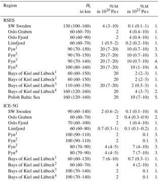
Further evaluation of our results is enabled by comparison of calculated sea-level curves from the best-fitting regional earth models to RSL data used. Figure 4 presents sea-level curves at eight selected locations. In the Oslo Fjord and in

-20 -15 -10 -5 0 5

Land uplift [m]

0 3 6 9 12

Time BP [ka] Oldenburger Graben

-20 -15 -10 -5 0 5

0 3 6 9 12

Time BP [ka] Redentin

-20 -15 -10 -5 0 5

0 3 6 9 12

Time BP [ka] Korkwitz -5

0 5 10 15

Land uplift [m]

0 3 6 9 12

Limfjord

-20 -15 -10 -5 0 5

0 3 6 9 12

Hiddensee 0

50 100 150 200 250

Land uplift [m]

0 3 6 9 12 15

Oslo Fjord

0 20 40 60 80 100

0 3 6 9 12 15

HK

-20 -15 -10 -5 0 5

0 3 6 9 12

Poland

RSES Ice-5G

Fig. 4. Comparison of RSL data (red dots) at selected locations to sea-level curves as calculated with the best earth model for a respective region and ice model RSES (Lambeck et al., 1998, blue) and ICE-5G (Peltier, 2004, green).

Figure 4. Comparison of RSL data (red dots) at selected locations

to sea-level curves as calculated with the best earth model for a respective region and ice model RSES (Lambeck et al., 1998, blue) and ICE-5G (Peltier, 2004, green).

SW Sweden (HK, the archaeological data from Hensbacka culture sites), there is a very good fit between observations and the modelled curves. The RSL data from Limfjord in northern Denmark are not fitted well, but one has to note that there is only small variation of about 5 m in 5000 years in this data set, which is hard to trace for the model. Along the Ger-man Baltic Sea coast, this variation is much larger and thus better fits can be achieved. In Hiddensee both RSES and ICE-5G ice models result in a good match of the sea-level data, but partly outside the given error bars of the RSL data. In the Oldenburger Graben and Redentin, the RSES ice model traces the RSL data better than ICE-5G, while in Körkwitz the ICE-5G ice model performs better than RSES. In Poland both ice models predict the sea-level rise well. Our compison shows that although good fits are achieved in some ar-eas, each ice model cannot perfectly fit all data, and some sea-level curves as predicted by the models lie outside the error bars of the observations. Errors in the ice model affect the behaviour of calculated sea-level curves and may lead to a worse misfit, which eventually alters the confidence ranges in Fig. 3. This does not necessarily mean that another earth model would be preferred, but the RSL curve of this earth– ice model combination is disarranged.

(9)

Table 2. Overview of three-layer 1-D earth models derived for regional RSL data subsets in the southern Baltic Sea.Hllithospheric thickness,

ηUMupper-mantle viscosity,ηLMlower-mantle viscosity,χmisfit.∗This regional result from Lambeck et al. (1998) contains additional RSL

data that were considered to be less satisfactory by Lambeck et al. (1998).

Region Reference Ice Hl ηUM ηLM

model in km in 1020Pa s in 1022Pa s SW Sweden this study RSES 130 4 0.1 this study ICE-5G 90 2 0.1 Lambeck et al. (1998) RSES 50 2.5 3

∗ _{Lambeck et al. (1998)} _RSES ₈₀ ₁ ₁

Oslo Fjord this study RSES 60 2 4 this study ICE-5G 70 2 1 Lambeck et al. (1998) RSES 80 1.5 3 Fyn this study RSES 90 20 10 this study ICE-5G 100 2 0.1 (Denmark) Lambeck et al. (1998) RSES 150 4 3

three subsets with available data: Oslo Fjord, SW Sweden and Denmark. This choice is similar to our study, but the SW Sweden data set from Lambeck et al. (1998) did not contain RSL data from the Hensbacka sites and their Dan-ish data set contained data from the Great Belt and the Limfjord. For Oslo Fjord, the authors found a 80 km thick lithosphere and an upper-mantle viscosity of 1.5×1020Pa s with an older version of the RSES ice model (Table 2). In SW Sweden lithospheric thickness of 50 km thickness was 30 km thinner than that of Oslo Fjord. Upper-mantle vis-cosity is here slightly higher at 2.5×1020Pa s. Higher val-ues were found in Denmark. Lithospheric thickness was determined to be 150 km and upper-mantle viscosity with 4×1020Pa s. While these results confirm the thicker litho-sphere in Denmark/Rinkøping-Fyn High as well as the upper-mantle viscosities of our study, the differences be-tween SW Sweden and the Oslo Fjord are large both in the lithospheric thickness estimate and also in the structural im-plications. These differences can be explained due to our slightly different grouping, the new data in the SW Sweden subset and the usage of an updated version of RSES that was available to us.

We note in this regard that Kaufmann and Wu (2002) showed that if the ice-load history is known, then it is only possible to accurately estimate lateral changes in lithospheric thickness with 1-D earth models and regional RSL data sub-sets if there is no lateral change in mantle viscosity below the lithosphere. Otherwise the inferred lateral variations in litho-spheric thickness can only be estimated qualitatively. This condition is not met with our RSES ice-load history and thus these results have to be cautiously interpreted. ICE-5G shows smaller variations in upper-mantle viscosity for each region than RSES; therefore, these results are more reliable in view of the findings by Kaufmann and Wu (2002). However, the results from ICE-5G do not agree with seismological results,

which show large increase in lithospheric thickness towards the east.

To further evaluate this, we therefore turn to the litho-sphere models derived from seismological data and com-pare them to our results. Gregersen et al. (2002) provided a NE–SW profile from southern Sweden to central Ger-many based on P-wave velocity perturbation. The general-ized profile shows a 300 km thick lithosphere northeast of the Teisseyre–Tornquist Zone, but we note that the lower bound-ary cannot be clearly defined due to the relatively high ve-locities in the upper mantle. Therefore, the lithosphere might be thinner than 300 km. The lithospheric thickness then de-creases to about 125 km between the Rinkøping-Fyn High and the Teisseyre–Tornquist Zone in Denmark, and about 80 km southwest of the Rinkøping-Fyn High in Germany.

Tesauro et al. (2009) showed a map of thermal lithospheric thickness in Europe south of 60◦N latitude. The model is based on the inversion of a tomography model of Koulakov et al. (2009) and was provided to us in a 0.25×0.25 degree grid. In southern Sweden, they find a thickness exceeding 180 km (Fig. 5a, isolines). The thickness then decreases to about 120 km in northeastern Germany. In the southern North Sea, they find an average of about 135 km for Belgium and about 110 km for the Netherlands and northwest Germany. A comparison with receiver function data mirrored the lat-eral variation (Tesauro et al., 2009), and visual comparison with newer S-receiver function results (Geissler et al., 2010) supports the results as well. The British Isles have varying thicknesses between 100 and 180 km.

(10)

5˚ 10˚ 15˚ 20˚ 25˚ 52˚

54˚ 56˚ 58˚ 60˚

160

170

180

180 200 2

20

220

240

260280

B

5˚ 10˚ 15˚ 20˚ 25˚52˚

54˚ 56˚ 58˚ 60˚

110 120

120

130

140

150 160170180 200 220

240

260 C

5˚ 10˚ 15˚ 20˚ 25˚

52˚ 52˚

54˚ 54˚

56˚ 56˚

58˚ 58˚

60˚ 60˚

110

12₀

120

130 130

140 140

150

150 160

160

170

180

200

220

A

60 70 80 90 100 110 120 130 140 150 160

km

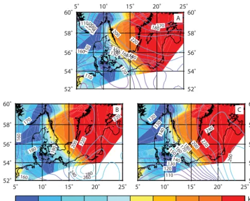
Figure 5. Comparison of calculated regional lithospheric thickness

variations with the RSES ice model (filled contour maps) to seis-mically and thermally derived lithospheric thicknesses (solid lines) by (A) Tesauro et al. (2009), (B) Hamza and Vieira (2012) and (C) Priestley and McKenzie (2013). Contour maps are drawn with the GMT pscontour function.

Recently, Priestley and McKenzie (2013) introduced a 2×2 degree seismologically determined lithosphere model that also includes thermal information. They combined a sur-face wave tomography model with temperature (ocean and continents) and pressure (continents) estimates to generate shear-wave velocity estimates. These estimates and a de-scription of their relaxation behaviour at high temperatures is then used to infer the lithospheric thickness. In the south-ern Baltic Sea area, there are two major structural features (Fig. 5c, isolines). First, lithospheric thickness decreases from 260 km in the east to 110–120 km in the west. The gra-dient is almost constant, but slightly steeper in SW Sweden. Second, from western central Denmark towards the North Sea, an area encompassing the Rinkøping-Fyn High, litho-spheric thickness remains at an almost constant level of about 140 km. To the north and south it drops to about 110 km.

Figure 5 shows our results for the best lithospheric thick-ness estimates with the RSES ice model as coloured maps, with the additional estimates from Steffen and Kaufmann (2005) for Fennoscandia and from Vink et al. (2007) for the southern North Sea to give a more complete overview on GIA-inferred lithospheric thickness. We do not compare our ICE-5G results as (i) they do not show the pronounced thickness increase to the east and (ii) Steffen and Kaufmann (2005) and Vink et al. (2007) did not provide results for this ice model which would allow a comparison in the North Sea and central Fennoscandia. The GIA-inferred lithospheric thickness map is drawn using the GMT pscontour function (Wessel and Smith, 1998) by assigning the lithospheric thick-ness values of the best-fitting earth model for each region to

the coordinates of each RSL data sample location. The re-sults of Tesauro et al. (2009, A), Hamza and Vieira (2012, B) and Priestley and McKenzie (2013, C) are overlain with con-tour lines. In the south and east of the area shown no results exist for the GIA-inferred lithospheric thickness.

In general, the seismically and thermally inferred litho-spheric thickness values do not show a good match to our GIA-model results. All these models show lithospheric thick-nesses of at least 110 km in the area under investigation. Also, their maximum values exceed 200 km considerably. However, we note that these three lithosphere models also do not show a good fit to each other either, except for the general increase from west to east. The thicker lithospheres of the seismological and/or thermal models is due to the fact that a different timescale is addressed. Seismological results are related to observations and processes of seconds to minutes, while the GIA-inferred lithosphere is related to a process of 100 ka. Nonetheless, relative differences should agree.

The thickness according to Hamza and Vieira (2012) has a pronounced peak of 280 km in Poland and also shows de-creasing values from east to west with no distinct change in the gradient except a kind of plateau with about 180 km in northwestern Denmark. Except the decrease in lithospheric thickness from east to west, there is no other similar feature when compared to our GIA-model results.

The lithospheric thickness by Tesauro et al. (2009) reaches its highest value of 220 km in a broad band from southeastern Sweden to Latvia. It also shows decreasing values from east to west; however, the gradient is much steeper at the south-western Swedish coast. It thins to 150 km towards the north-west of Denmark, and then becoming thicker again. To the north and south of this area values drop to less than 110 km. There is a structural agreement in the form of the east–west decrease. The Rinkøping-Fyn High appears to lie further north in the thermal lithosphere. The thin GIA-lithosphere along the German Baltic Sea coast agrees with the plateau of 120 km in the thermal lithosphere. The structure of the Oslo Graben cannot be distinguished.

The best agreement of GIA-modelling-derived values is probably found in comparison to the new model by Priest-ley and McKenzie (2013). Both the EW-decrease trend and the location of the Rinkøping-Fyn High fit structurally well. Small differences are found in the northwest of our investi-gation area and in the German Bight. However, we also have to note that the spatial resolution of this model is two degrees and thus smaller features may not be clearly identified.

6 Conclusions

(11)

for the first time. We employed the software ICEAGE and two different global ice models.

However, we made several assumptions and there are cer-tain conditions to be kept in mind that may lead to different results in future investigations: we use ice models that are related to a certain earth model, and thus they are already bi-ased by a certain lithospheric thickness and mantle viscosity. Our earth model is based on Maxwell rheology. Furthermore, it is possible that the ice models have imperfections that are absorbed by a wrong earth model, but anyhow lead to a good fit to the observations. We also note that variation in litho-spheric thickness for regional subsets can only be clearly de-termined when mantle viscosity in each region is about con-stant (Kaufmann and Wu, 2002). This condition is not met for all regions. It is therefore possible that a 3-D earth model for the southern Baltic Sea with a different radial earth struc-ture in each subregion than our determined 1-D earth models fits much better than a combination of all our 1-D models. All these items can increase the confidence regions of our study.

Within our calculated confidence levels, the following re-sults were determined. The lithospheric thickness varies from 60 km in the Oslo Graben and the German Baltic Sea coast to up to 160 km in Poland. When only the best-fitting litho-sphere is analysed, we see a trend to thicker litholitho-sphere from west to east using the RSES ice model, but this is less pro-nounced with ICE-5G. The Rinkøping-Fyn High in between the Oslo Graben and Germany is at least 30 km thicker than the surrounding areas in the north and south. However, the confidence levels of the lithosphere are so large that an ac-curate determination is not possible. The variation in litho-spheric thickness based on RSES agrees to a certain extent, when compared visually, to thickness models based on seis-mological and/or thermal investigation. A direct comparison of thicknesses is not possible due to the different definitions of lithosphere in seismological/thermal and GIA investiga-tions.

Upper-mantle viscosity is about [2–7]×1020Pa s in the Oslo Graben and SW Sweden and thus confirms values found for Fennoscandia, the British Isles and the southern North Sea previously. In the southern Baltic Sea, similar values are obtained with ICE-5G, but we note quite high values of 2×1021Pa s for this region when using the RSES ice his-tory. Bifurcation indicates that lower values in the range of [4–10]×1020Pa s are likely. As expected, lower-mantle vis-cosity cannot be sufficiently determined.

Future investigations with hopefully more RSL data in the southern Baltic Sea and an updated ice model (both tested ice models have experienced major recent improvements, but these revised versions have not been published yet) may help to further confirm the results herein with smaller confidence regions than ours and also overcome the differences between the results from the two ice models in certain areas. However, it will not be possible to add RSL data in the southern Baltic Sea which are older and deeper than the ones used in our

study as the Pleistocene relief with the threshold of 25 m in the Great Belt did not allow an earlier deposition.

Acknowledgements. We are grateful for the excellent reviews

by Wouter van der Wal and Patrick Wu that helped improve the paper. We would like to thank Kurt Lambeck (Research School of Earth Sciences, Australian National University) and Magdala Tesauro (GFZ Potsdam) for kindly providing the RSES ice model and the thermal lithosphere model in central and southern Europe, respectively. Figures were prepared using GMT software (Wessel and Smith, 1998).

Special Issue: “Lithosphere-cryosphere interactions”

Edited by: M. Poutanen, B. Vermeersen, V. Klemann, and C. Pascal

References

Artemieva, I. M.: The continental lithosphere: Reconciling thermal, seismic, and petrologic data, Lithos, 109, 23–46, doi:10.1016/j.lithos.2008.09.015, 2009.

Bennike, O., Jensen, J. B., Lemke, W., Kuijpers, A., and Lomholt, S.: Late- and postglacial history of the Great Belt, Denmark, Boreas, 33, 18–33, doi:10.1111/j.1502-3885.2004.tb00993.x,2004.

Bitinas, A., Damušyte, A., Hütt, G., Martma, T., Ruplenaite, G., Stanˇcikaite, M., ¯Usaityte, D., and Vaikmäe, R.: Stratigraphic correlation of Late Weichselian and Holocene Deposits in the Lithuanian coastal region, P. Est. Acad. Sci.-Geol., 49, 200–217, 2000.

Bitinas, A., Damušyte, A., Stanˇcikaite, M., and Aleksa P.: Geologi-cal development of the Nemunas River Delta and adjacent areas, West Lithuania, Geological Quarterly, 46, 375–389, 2002. Christensen, Ch., Fischer, A., and Mathiassen, D. R.: The great sea

rise in the Storebælt, in: The Danish Storebælt since the Ice Age – man, sea and forest, edited by: Pedersen, L., Fischer, A., and Aaby, B., A/S Storebælt Fixed Link, Copenhagen, 45–54, 1997. Dèzes, P., and Ziegler, P. A.: Moho depth map of Western and Cen-tral Europe, avfailable at: https://comp1.geol.unibas.ch/, 2002. Dziewonski, A. M. and Anderson D. L.: Preliminary

refer-ence Earth model, Phys. Earth Planet. Inter., 25, 297–356, doi:10.1016/0031-9201(81)90046-7, 1981.

Eaton, D. W., Darbyshire, F., Evans, R. L., Grütter, H., Jones, A. G., and Yuan, X.: The elusive lithosphere-asthenosphere boundary (LAB) beneath cratons, Lithos, 109, 1– 22, doi:10.1016/j.lithos.2008.05.009, 2009.

Farrell, W. E. and Clark, J. A.: On postglacial sea level, Geophys. J. R. Astr. Soc., 46, 647–667, doi:10.1111/j.1365-246X.1976.tb01252.x, 1976.

Fjeldskaar, W.: Viscosity and thickness of the asthenosphere de-tected from the Fennoscandian uplift, Earth Planet. Sci. Lett., 126, 399–410, doi:10.1016/0012-821X(94)90120-1, 1994. Geissler, W. H., Sodoudi, F., and Kind, R.: Thickness of the

cen-tral and eastern european lithosphere as seen by S receiver functions, Geophys. J. Int., 181, 604–634, doi:10.1111/j.1365-246X.2010.04548.x, 2010.

(12)

Sweden, Tectonophysics, 360, 61–73, doi:10.1016/S0040-1951(02)00347-5, 2002.

Hamza, V. M. and Vieira, F. P.: Global distribution of the lithosphere-asthenosphere boundary: a new look, Solid Earth, 3, 199–212, doi:10.5194/se-3-199-2012, 2012.

Hoffmann, G., Schmedemann, N., and Schafmeister, M.-Th.: Rela-tive sea-level curve for SE Rügen and Usedom Island (SW Baltic Sea coast, Germany) using decompacted profiles, Z. dtsch. Ges. Geowiss., 160, 69–78, 2009.

Hofmann, W. and Winn, K.: The Littorina Transgression in the Western Baltic Sea as indicated by subfossil Chi-ronomidae (Diptera) and Cladocera (Crustacea), Int. Rev. Hydrobiol., 85, 267–291, doi:10.1002/(SICI)1522-2632(200004)85:2/3<267::AID-IROH267>3.0.CO;2-Q, 2000. Jakobsen, O.: Die Grube-Wesseker Niederung (Oldenburger

Graben, Ostholstein): Quartärgeologische und geoarchäologis-che Untersuchungen zur Landschaftsgeschichte vor dem Hin-tergrund des anhaltenden postglazialen Meeresspiegelanstiegs, PhD.-Thesis, Univ. Kiel, 190 pp., 2004.

Kaufmann, G.: Program package ICEAGE, Version 2004, Manuscript, Institut für Geophysik der Universität Göttingen, 40 pp., 2004.

Kaufmann, G. and Wu, P.: Glacial isostatic adjustment in Fennoscandia with a three-dimensional viscosity structure as an inverse problem, Earth Planet. Sci. Lett., 197, 1–10, doi:10.1016/S0012-821X(02)00477-6, 2002.

Koulakov, I., Kaban, M. K., Tesauro, M., Cloetingh, S.: P and S velocity anomalies in the upper mantle beneath Europe from to-mographic inversion of ISC data, Geophys. J. Int., 179, 345–366, doi:10.1111/j.1365-246X.2009.04279.x, 2009.

Lambeck K., Smither, C., and Johnston, P.: Sea-level change, glacial rebound and mantle viscosity for northern Europe, Geophys. J. Int., 134, 102–144, doi:10.1046/j.1365-246x.1998.00541.x, 1998.

Lampe, R., Meyer, H., Ziekur, R., Janke, W., and Endtmann, E.: Holocene evolution of an irregularly sinking coast and the inter-actions of sea-level rise, accumulation space and sediment sup-ply, Bericht der Römisch-Germanischen Kommission, 88, 15– 46, 2007.

Lampe, R., Endtmann, E., Janke, W., and Meyer, H.: Relative sea-level development and isostasy along the NE German Baltic Sea coast during the past 9 ka, Quaternary Sci. J., 59, 3–20, doi:10.3285/eg.59.1-2.01, 2011.

Lange, W. and Menke, B.: Beiträge zur frühpostglazialen erd-und vegetationsgeschichtlichen Entwicklung im Eidergebiet, ins-besondere zur Flußgeschichte und zur Genese des sogenannten Basistorfes, Meyniana, 17, 29–44, 1967.

Lübke, H., Schmölcke, U., and Tauber, F.: Mesolithic Hunter-Fishers in a Changing World: a case study of submerged sites on the Jäckelberg, Wismar Bay, northeastern Germany, in: Sub-merged Prehistory, edited by: Benjamin, J., Bonsall, C., Pickard, C., and Fischer, A., 21–37, Oxbow Books, Oxford, 2011. Mitrovica, J. X., and Milne, G. A.: Glaciation-induced perturbations

in the Earth’s rotation: a new appraisal, J. Geophys. Res., 103, 985–1005, doi:10.1029/97JB02121, 1998.

Mitrovica, J. X., Davis, J. L., and Shapiro, I. I.: A spectral for-malism for computing three–dimensional deformations due to surface loads 1. Theory, J. Geophys. Res., 99, 7057–7073, doi:10.1029/93JB03128, 1994.

Peltier, W. R.: Global glacial isostasy and the surface of the Ice-Age Earth: the ICE-5G (VM2) model and GRACE, Annu. Rev. Earth Pl. Sc., 32, 111–149, doi:10.1146/annurev.earth.32.082503.144359, 2004.

Petit, J. R., Jouzel, J., Raynaud, D., Barkov, N. I., Barnola, J. M., Basile, I., Bender, M., Chappellaz, J., Davis, J., Delaygue, G., Delmotte, M., Kotlyakov, V. M., Legrand, M., Lipenkov, V., Lo-rius, C., Pépin, L., Ritz, C., Saltzman, E., and Stievenard, M.: Climate and Atmospheric History of the Past 420,000 years from the Vostok Ice Core, Antarctica, Nature, 399, 429–436, doi:10.1038/20859, 1999.

Priestley, K. and McKenzie, D.: The relationship between shear wave velocity, temperature, attenuation and viscosity in the shal-low part of the mantle, Earth Planet. Sci. Lett., 381, 78–91, doi:10.1016/j.epsl.2013.08.022, 2013.

Rößler, D., Moros, M., and Lemke, W.: The Littorina transgres-sion in the southwestern Baltic Sea: new insights based on proxy methods and radiocarbon dating of sediment cores„ Boreas, 40, 231–241, doi:10.1111/j.1502-3885.2010.00180.x, 2011. Scheck-Wenderoth, M., and Lamarche, J.: Crustal memory and

basin evolution in the Central European Basin System – new in-sights from a 3D structural model, Tectonophysics, 397, 143– 165, doi:10.1016/j.tecto.2004.10.007, 2005.

Schmitt, L., Larsson, S., Burdukiewicz, J., Ziker, J., Svedhage, K., Zamon, J., Steffen, H.: Chronological insights, cultural change, and resource exploitation on the west coast of Sweden during the Late Paleolithic/early Mesolithic transition, Oxford J. Arch., 28, 1–27, doi:10.1111/j.1468-0092.2008.00317.x, 2009.

Steffen, H. and Kaufmann, G.: Glacial isostatic adjustment of Scandinavia and northwestern Europe and the radial viscosity structure of the Earth’s mantle, Geophys. J. Int., 163, 801–812, doi:10.1111/j.1365-246X.2005.02740.x, 2005.

Steffen, H. and Wu, P.: Glacial isostatic adjustment in Fennoscan-dia – A review of data and modeling, J. Geodyn., 52, 169–204, doi:10.1016/j.jog.2011.03.002, 2011.

Steffen, H., Kaufmann, G., and Wu, P.: Three-dimensional finite-element modelling of the glacial isostatic adjustment in Fennoscandia, Earth Planet. Sci. Lett., 250, 358–375, doi:10.1016/j.epsl.2006.08.003, 2006.

Steffen, H., Wu, P., and Wang, H. S.: Determination of the Earth’s structure in Fennoscandia from GRACE and implications on the optimal post-processing of GRACE data,Geophys. J. Int., 182, 1295–1310, doi:10.1111/j.1365-246X.2010.04718.x, 2010. Tauber, F.: Seafloor exploration with sidescan sonar for

geo-archaeological investigations, Berichte der Römisch-Germanischen Kommission, 88, 67–79, 2007.

Tesauro, M., Kaban, M. K., and Cloetingh, S. A. P. L.: A new ther-mal and rheological model of the European lithosphere, Tectono-physics, 476, 478–495, doi:10.1016/j.tecto.2009.07.022, 2009. U´scinowicz, S.: Relative sea level changes, glacio-isostatic rebound

and shoreline displacement in the Southern Baltic, Polish Geo-logical Institute Special Papers, 10, 1–80, 2003.

van der Wal, W., Barnhoorn, A., Stocchi, P., Gradmann, S., Wu, P., Drury., M., and Vermeersen, L. L. A.: Glacial Isostatic Adjust-ment Model with Composite 3D Earth Rheology for Fennoscan-dia, Geophys. J. Int., 194, 61–77, doi:10.1093/gji/ggt099, 2013. Vink, A., Steffen, H., Reinhardt L., and Kaufmann, G.: Holocene

(13)

the Netherlands, Germany, southern North Sea), Quat. Sci. Rev., 26, 3249–3275, doi:10.1016/j.quascirev.2007.07.014, 2007. Wang, H. S., Wu, P., and van der Wal, W.: Using postglacial sea

level, crustal velocities and gravity-rate-of-change to constrain the influence of thermal effects on mantle lateral heterogeneities, J. Geodyn., 46, 104–117, doi:10.1016/j.jog.2008.03.003, 2008. Wessel, P. and Smith, W. H. F.: New, improved version of

generic mapping tools released, EOS Trans. AGU, 79, p. 579, doi:10.1029/98EO00426, 1998.

Winn, K., Averdieck, F.-R., Erlenkeuser, H. and Werner, F.: Holocene sea level rise in the western Baltic and the question of isostatic subsidence, Meyniana, 38, 61–80, 1986.

Wu, P., Wang, H. S., and Schotman, H.: Postglacial induced sur-face motions, sea levels and geoid rates on a spherical, self-gravitating laterally heterogeneous earth, J. Geodyn., 39, 127– 142, doi:10.1016/j.jog.2004.08.006, 2005.

Wu, P., Wang, H., and Steffen, H.: The role of thermal effect on mantle seismic anomalies under Laurentia and Fennoscandia from observations of Glacial Isostatic Adjustment, Geophys. J. Int., 192, 7–17, doi:10.1093/gji/ggs009, 2013.