www.the-cryosphere.net/10/2191/2016/ doi:10.5194/tc-10-2191-2016
© Author(s) 2016. CC Attribution 3.0 License.
Mechanism of seasonal Arctic sea ice evolution and Arctic
amplification
Kwang-Yul Kim1, Benjamin D. Hamlington2, Hanna Na3, and Jinju Kim1
1School of Earth and Environmental Sciences, Seoul National University, Seoul 08826, Republic of Korea
2Department of Ocean, Earth and Atmospheric Sciences, Old Dominion University, Norfork, Virginia 23529, USA 3Ocean Circulation and Climate Research Center, Korea Institute of Ocean Science and Technology,
Ansan, 15627, Republic of Korea
Correspondence to:Kwang-Yul Kim (kwang56@snu.ac.kr)
Received: 15 March 2016 – Published in The Cryosphere Discuss.: 29 April 2016 Revised: 28 June 2016 – Accepted: 8 September 2016 – Published: 22 September 2016
Abstract. Sea ice loss is proposed as a primary reason for the Arctic amplification, although the physical mechanism of the Arctic amplification and its connection with sea ice melting is still in debate. In the present study, monthly ERA-Interim reanalysis data are analyzed via cyclostationary em-pirical orthogonal function analysis to understand the sea-sonal mechanism of sea ice loss in the Arctic Ocean and the Arctic amplification. While sea ice loss is widespread over much of the perimeter of the Arctic Ocean in summer, sea ice remains thin in winter only in the Barents–Kara seas. Ex-cessive turbulent heat flux through the sea surface exposed to air due to sea ice reduction warms the atmospheric col-umn. Warmer air increases the downward longwave radia-tion and subsequently surface air temperature, which facili-tates sea surface remains to be free of ice. This positive feed-back mechanism is not clearly observed in the Laptev, East Siberian, Chukchi, and Beaufort seas, since sea ice refreezes in late fall (November) before excessive turbulent heat flux is available for warming the atmospheric column in winter. A detailed seasonal heat budget is presented in order to un-derstand specific differences between the Barents–Kara seas and Laptev, East Siberian, Chukchi, and Beaufort seas.
1 Introduction
Warming over the Arctic Ocean is observed to accelerate in recent decades. The rate of warming in the Arctic is more than twice the rate of globally averaged warming. This warm-ing and subsequent acceleration is referred to as Arctic
am-plification (Screen and Simmonds, 2010a, b; Serreze and Barry, 2011). Reduction of sea ice in the Arctic Ocean is suggested to have contributed to the accelerated warming in the lower troposphere (Holland and Bitz, 2003; Serreze et al., 2009; Kumar et al., 2010; Screen and Simmonds, 2010a, b). The rate of sea ice loss in the Barents and Kara seas ap-pears to have increased significantly over the last 2 decades in comparison to that in the earlier period (Stroeve et al., 2007; Comiso et al., 2008; Serreze et al., 2009; Cavalieri and Parkinson, 2012). As should be expected, the accelerated loss of sea ice in the Arctic Ocean has a profound impact on the heat energy budget, sea ice stability, carbon cycle feedback, and atmospheric and oceanic circulation locally and remotely (IPCC, 2013, Serreze and Barry, 2011).
Another mechanism proposed is the water vapor feedback (Francis and Hunter, 2006; Sedlar et al., 2011; Park et al., 2015). As warming increases, water vapor content in the at-mospheric column increases, leading to an amplified green-house effect. Longwave radiation is trapped more in the at-mospheric column, resulting in warming of the atat-mospheric column. In a similar sense, the increased cloudiness due to increased amount of water vapor leaving sea surface may re-sult in an amplification of lower tropospheric warming (Fran-cis and Hunter, 2007).
The most widely accepted mechanism for Arctic ampli-fication is the “insulation feedback”. When sea surface mains to be free of ice in winter, turbulent heat flux is re-leased from the open ocean surface, which is instrumental for warming the lower troposphere (Francis et al., 2009; Serreze et al., 2009; Screen and Simmonds, 2010a, b; Deser et al., 2010; Overland et al., 2011; Serreze and Barry, 2011; Cohen et al., 2014; Screen et al., 2014). According to this hypothe-sis, increased reception of insolation through the sea surface exposed to air in summer keeps the sea surface warmer and is released in fall and early winter, making the atmosphere warmer. Through this so-called “delayed warming”, sea sur-face remains to be ice free in fall and winter, and excessive turbulent heat flux becomes available through the open sea surface in winter.
It is not clear, however, why such a mechanism is readily seen only in the Barents and Kara seas but not in other areas of the Arctic (Petoukhov and Semenov, 2010; Screen and Si-monds, 2010b). While summer sea ice melting is clearly seen in areas other than the Barents and Kara seas, Arctic ampli-fication is observed only in the latter area in winter. Further, the role and contribution of increased absorption of insola-tion in summer for increased sea ice loss in winter is not clear, primarily because the region of winter sea ice reduc-tion and that of increased insolareduc-tion recepreduc-tion do not match closely. Thus, it is necessary to understand each term of the feedback process not only from a physical perspective but also in a quantitative one. An accurate quantitative estima-tion of each term of the feedback process may provide a clearer insight and yield a more convincing physical mecha-nism for the feedback process and a reasonable explanation for the regional difference in the Arctic Ocean. Considering the importance of sea ice loss in the overall energy budget and atmospheric and oceanic circulation in the Arctic region, it is also crucial to understand how fast Arctic amplification progresses.
One key issue to be dealt with in the present study is the mechanism of Arctic amplification. Cyclostationary empir-ical orthogonal function (CSEOF) analysis is carried out to identify detailed and physically consistent seasonal evolution patterns of physical variables associated with sea ice loss in the Arctic Ocean. Specifically, the physical mechanism of sea ice reduction and Arctic amplification is investigated from both a spatial and temporal standpoint, so that any delayed response can be explicitly considered. Quantification of each
term in the feedback process is attempted in order to clarify their relative importance in the feedback. Further, the role of water vapor and cloud in the feedback process is assessed. Another key issue to be addressed is why and how sea ice loss in winter develops in the Barents and Kara seas but not in the Laptev and Chukchi seas. This issue is important in order to understand the key components of and reduce uncer-tainty in the feedback process. Also, it is pivotal to determine how fast the Arctic amplification progresses. The rate of ac-celeration of the Arctic amplification is estimated based on CSEOF analysis.
2 Data and method of analysis
The dataset used in the present study is the ERA-Interim 1.5◦×1.5◦monthly reanalysis (Dee et al., 2011) from 1979
to 2014. Surface variables analyzed in the present study in-clude sea surface temperature, sea ice concentration, latent and sensible heat fluxes, upward and downward longwave and shortwave radiations, and 2 m air temperature. Pressure-level variables analyzed include air temperature, geopoten-tial, zonal wind, meridional wind, and specific humidity. Low-level and total cloud fractions are also analyzed.
The analysis tool employed in this study is the CSEOF technique (Kim et al., 1996, 2015; Kim and North, 1997). In CSEOF analysis, dataT (r, t )are decomposed in the form
T (r, t )=X
nBn(r, t ) Tn(t ), (1)
whereBn(r, t )are mutually orthogonal CSEOF loading
vec-tors (CSLVs) andTn(t )are mutually uncorrelated principal
component (PC) time series of variableT (r, t ). As in empir-ical orthogonal function (EOF) analysis, a main motivation of CSEOF analysis is to decompose variability into uncorre-lated and orthogonal components in order to understand ma-jor constituents of variability inT (r, t ). Unlike EOF loading vector, which is a spatial pattern, CSLV is a function of space and time describing temporal evolution pertaining to a phys-ical process inT (r, t ). Further, CSLV is periodic in time:
Bn(r, t )=Bn(r, t+d), (2)
where the periodicitydis called the nested period. This peri-odicity derives from the cyclostationary assumption that the statistics ofT (r, t )is periodic. For example, space–time co-variance function ofT (r, t )is defined by
C r, t;r0, t0
=< T (r, t )T (r0, t0) >=C(r, t+d;r0, t0+d). (3) CSEOF loading vectors are derived as eigenvectors of pe-riodic space–time covariance function by solving
C r, t;r0, t0·Bn r0, t0=λnBn(r, t ), (4)
whereBn(r, t ) are eigenvectors and λn are eigenvalues of
periodicity of space–time covariance function, correspond-ing eigenvectors are also periodic with the same periodicity. Detailed solution procedures for CSEOF loading vectors are beyond the scope of this paper and can be found in Kim et al. (1996) and Kim and North (1997).
As in EOF analysis, CSLVs are mutually orthogonal and PC time series are uncorrelated. That is,
(Bm(r, t )·Bn(r, t ))
= 1 N d
XN r=1
Xd
t=1Bm(r, t )Bn(r, t )=δnm, (5) and
(Tm(t )·Tn(t ))=
1
M
XM
t=1Tm(t ) Tn(t )=λnδnm. (6) Here(A·B)denotes dot (inner) product betweenAandB,
N is the number of spatial points,Mis the number of tempo-ral points, andλn, called eigenvalue, represents the variance
of PC time seriesTn(t ). Thus, CSLVs are interpreted as
mu-tually orthogonal space–time evolution in the data, of which the amplitude (PC) time series are mutually uncorrelated. In fact, EOF analysis is a special case of CSEOF analysis with the nested periodd=1. Thus, each loading vector consists of one spatial pattern and can be found from a spatial covariance function. Sometimes, a different normalization convention is used, i.e.,
(Bm(r, t )·Bn(r, t ))=λnδnm, (7)
and
(Tm(t )·Tn(t ))=δnm. (8)
This normalization convention is used in the present study. It is often important to examine several variables to un-derstand the details of a physical process. A second variable
P (r, t )is similarly decomposed into
P (r, t )=X
nCn(r, t ) Pn(t ). (9)
In general, there is no one-to-one correspondence between
{Tn(t )}and{Pn(t )}. This means that{Bn(r, t )}and{Cn(r, t )}
are not physically consistent. In order to make physical evo-lutions derived from two variables to be consistent, P (r, t )
should be written as
P (r, t )=X
nC (r)
n (r, t ) Tn(t ), (10)
whereCn(r)(r, t )is a new set of loading vectors with
corre-sponding PC time series {Tn(t )}. In other words, two sets
of loading vectors, nBn(r, t ) , Cn(r)(r, t )
o
, are governed by identical PC time series. The loading vectors Bn(r, t )and
Cn(r)(r, t )represent an identical physical process manifested
in two different variables.
Table 1.Variables used in the present study with units andR2 val-ues of regression. The target variable for regression is 2 m air tem-perature.
Variable R2value
Sea ice (fraction) 0.960
Sea surface temperature (◦C) 0.937
Downward longwave radiation (W m−2) 0.995
Upward longwave radiation (W m−2) 0.999
Net shortwave radiation (W m−2) 0.907
Sensible heat flux (W m−2) 0.968
Latent heat flux (W m−2) 0.954
Low cloud cover (fraction) 0.947
Total cloud cover (fraction) 0.921
Specific humidity (g kg−1) 0.945
Air temperature (1000–850 hPa;◦C) 0.962
Geopotential (1000–850 hPa; m2s−2) 0.772
Wind (1000–850 hPa; m s−1) 0.844
The new set of loading vectors can be determined via the so-called regression analysis in CSEOF space (Kim et al., 2015). It is a two-step process:
Tn(t )=
XM
m=1α
(n)
m Pm(t )+ε(n)(t ), (11)
and
Cn(r)(r, t )=XM
m=1α
(n)
m Cm(r, t ), n=1,2,· · ·, (12)
where M is the number of PC time series used for mul-tivariate regression andε(n)(t )is regression error time se-ries. In this study, 20 PC time series are used for regression (M=20). The variableT (r, t )is called the target variable and is determined in such a way that the physical process under investigation is clearly identified and separated as a single CSEOF mode. TheR2value measures the accuracy of regression in Eq. (11). Namely,
R2=1− var(εn(t ))var(Tn(t )). (13)
Thus,R2value close to unity implies that variance of regres-sion error time series is very small compared to that of the target PC time series. As a result of regression analysis in CSEOF space, entire data (variables) can be written as Data(r, t )=
X n
n
Bn(r, t ) , Cn(r)(r, t ) , D (r) n (r, t ) , E
(r) n (r, t ) ,· · ·
o
Tn(t ), (14)
Sea ice concentration (%)
Barents & Barents & Kara Seas Kara Sea
s
Laptev Laptev Sea Sea
East East Siberian Siberian Sea Sea
Europe Europ
e
Russia
Russia Cana da Cana
da
Chukchi Chukchi Sea Sea
Beauf ort Beaufo
rt
Sea Sea Greenland
Gree nland
Figure 1.Geography of the Arctic Ocean (69–90◦N) and the sea-sonal patterns of average sea ice concentration (%) based on 1979– 2014 ERA-Interim data.
The nested period is set to 1 year in the present study. Therefore, each CSLV consists of 12 spatial patterns for each month of the year. As shown in Eq. (1), amplitude of each CSLV is governed by corresponding PC time series. Thus, the strength of evolution as depicted in curly braces in Eq. (14) varies on temporal scales longer than the nested period.
3 Results and discussion
Northern hemispheric (30–90◦N) 2 m air temperature is used as the target variable, since polar amplification in the North-ern Hemisphere is clearly identified as the leading mode in 2 m air temperature aside from the seasonal cycle. Then, CSEOF analysis followed by regression analysis is con-ducted on all other (predictor) variables to extract physically consistent space–time evolution patterns from these vari-ables. Table 1 shows theR2values of regression for different variables.
3.1 Seasonal patterns of sea ice concentration
Figure 1 shows the average seasonal patterns of sea ice con-centration in the Arctic Ocean. The sea ice boundary in the Atlantic sector appears to be most sensitive throughout the year. In the Russian and Canadian sectors of the Arctic Ocean, the ice boundary abuts the continents in winter and
(a) 2 m AIR T
(b)
Time (year)
Amplitude
Figure 2.The seasonal patterns of the northern hemispheric (30–
90◦N) warming mode (upper panel; 0.3 K) and the corresponding
amplitude time series (lower panel). The dashed curve is an expo-nential fit (see Eq. 8) to the PC time series.
spring but retreats to the north in summer and fall. During the melting season, sea ice concentration decreases signifi-cantly in the Laptev, East Siberian, Chukchi, and Beaufort seas.
3.2 The warming mode and associated anomalous patterns
Radiation
Figure 3.The regressed seasonal patterns of sea ice concentration
(shading; 1 %), net shortwave radiation (red contours;±1, 2, 4, 6,
8, 10 W m−2), and net longwave radiation (black contours;±0.5,
1, 2, 3, 4, 5 W m−2)in the Arctic region (64.5–90◦N). Net upward
longwave radiation and net downward shortwave radiation are de-fined as positive. Solid contours represent positive values and dotted contours represent negative values.
mode represents warming in the Northern Hemisphere. In particular, the PC time series shows a conspicuous trend dur-ing the study period, indicatdur-ing a persistent increase in SAT. Seasonal variation of the pattern and magnitude of warming is clear with significant warming in winter and weak warm-ing in summer. Other strikwarm-ing features include pronounced warming over the Barents–Kara seas in winter and weak cooling in East Asian midlatitudes (see also Fig. S2 in the Supplement). According to the PC time series, an accelera-tion of warming is obvious in the Arctic region, particularly over the Barents–Kara seas. In particular, 2006/07 warming in winter seems to have been unprecedented (Stroeve et al., 2008; Kumar et al., 2010).
Figure 3 shows the regressed seasonal patterns of sea ice concentration and radiation anomalies corresponding to the warming mode shown in Fig. 2. The anomalous pattern of sea ice concentration in winter looks similar to that in spring. However, the summer pattern looks similar to that in fall. In winter and spring, conspicuous decrease in sea ice concen-tration is primarily in the Barents–Kara seas, whereas sea ice melting is widespread in the Laptev, East Siberian, Chukchi, and Beaufort seas in summer and fall.
Surface flux
Figure 4.The regressed seasonal patterns of sea ice
concentra-tion (shading; 1 %), sensible heat flux (red contours;±1, 3, 5, 7,
10 W m−2), and latent heat flux (black contours;±0.2, 0.4, 0.6, 0.8,
1 W m−2)in the Arctic region (64.5–90◦N). Net upward heat flux
is defined as positive.
In winter, when insolation is weak, net longwave radiation is upward over the region of sea ice loss, while it is downward over much of the Arctic Ocean, particularly in the Atlantic sector. As sea ice decreases, warmer sea surface is exposed to air, yielding increased upward longwave radiation in the Barents–Kara seas. In the North Atlantic Ocean, where sea ice concentration is already low (Fig. 1), net longwave radi-ation is downward, suggesting that increase in atmospheric temperature is larger than that of sea surface temperature. In late spring (May), downward shortwave radiation increases significantly over the region of sea ice loss. The increase in shortwave radiation is much larger than the net longwave ra-diation, thereby resulting in net downward radiation flux over the region of sea ice loss. In summer, sea ice melting ex-pands into the Laptev, Chukchi, and Beaufort seas. There is little change in net longwave radiation, but downward short-wave radiation increases significantly over the region of sea ice loss. This marked increase in downward shortwave radi-ation in spring and summer is associated with the decreased albedo as open sea surface is exposed. In fall, the anomalous pattern of sea ice concentration is similar to that in summer, but the change in net longwave and shortwave radiation is small.
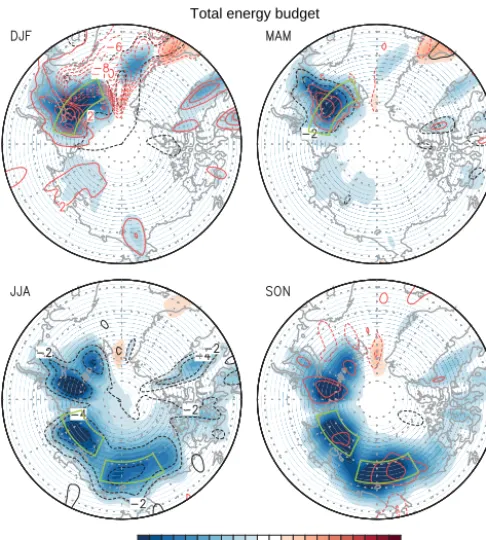
Total energy budget
Figure 5. The regressed seasonal patterns of sea ice
concentra-tion (shading; 1 %), net surface radiaconcentra-tion (black contours;±2, 4,
6, 8, 10 W m−2), and turbulent heat flux (red contours; ±2, 4,
8, 12, 16, 20 W m−2) in the Arctic region (64.5–90◦N).
Posi-tive values represent upward radiations and heat fluxes. The three green boxes represent the regions of significant change in sea ice
concentration: Barents and Kara seas (21–79.5◦E×75–79.5◦N),
Laptev Sea (105–154.5◦E×76.5–81◦N), and Chukchi Sea (165–
210◦E×72–76.5◦N).
to a lesser extent, latent heat flux increase over the Barents and Kara seas. Over the North Atlantic the anomalous sur-face flux is downward, primarily because of the increased atmospheric temperature; heat flux is reduced, since the dif-ference between sea surface temperature and air temperature is reduced due to atmospheric warming. In spring, a simi-lar increase in turbulent heat flux is clearly seen over the Barents–Kara seas. In summer, there is little change in tur-bulent heat flux although the area of sea ice melting is much expanded (Simmonds and Rudeva, 2012); note that there is little change in air temperature in summer (Fig. 2c). In fall, turbulent heat flux is increased primarily in the Kara and Chukchi seas because a wider area of sea surface is exposed to colder air above.
Figure 5 shows the seasonal patterns of anomalous net ra-diation and turbulent heat flux. In spring, net downward radi-ation and upward heat flux are similar in magnitude. In sum-mer, there is net downward radiation, which derives primar-ily from the increased absorption of solar radiation due to decreased albedo (Serreze and Francis, 2006; Serreze et al., 2009; Screen and Simmonds, 2010a; Screen and Simmonds,
2012). In fall heat flux is increased over the region of sea ice loss, but the amount of heat flux released is much less than the increased amount of shortwave radiation absorbed in summer. In winter, a significant increase in turbulent heat flux is observed over the Barents–Kara seas and a reduction of turbulent heat flux in the North Atlantic.
3.3 Seasonal patterns of sea surface temperature While sea surface temperature is observed to increase over the region of sea ice loss in summer and fall, anomalous sea surface temperature vanishes in the Laptev, East Siberian, Chukchi, and Beaufort seas as sea ice recovers over the area (Fig. 6). It should be pointed out that the increased net down-ward radiation in summer, and henceforth the increased sea surface temperature in summer and fall, does not lead to a pronounced thinning of sea ice in winter (see Fig. 6a). In-stead, sea ice loss is confined to the Barents–Kara seas in winter, where turbulent heat flux is significantly increased. It seems that the increased solar radiation as a result of albedo feedback is responsible for the sea ice loss and sea surface warming in summer, except for the western part of the Bar-ents Sea, where sea surface warming seems associated with oceanic heat transport. The increased energy, however, does not seem connected, at least directly, to the increased turbu-lent heat flux in winter. Note that the region of sea surface warming in summer does not match well with the region of sea ice loss in winter (Fig. 6).
3.4 Mechanism of sea ice loss
While significant loss is observed only during summer and fall over the Laptev and Chukchi seas, sea ice loss continues throughout the year over the Barents–Kara seas (see different regions of conspicuous sea ice loss in Fig. 5). In order to un-derstand why sea ice distribution differs markedly over the Barents and Kara seas, the monthly energy budget is com-puted in Fig. 7a. In April–June, absorption of shortwave ra-diation increases dramatically over the region; this excessive incoming energy explains the bulk of the total energy bud-get. During the rest of the year, net radiation change is fairly small (<3 W m−2). In contrast, turbulent energy is released mainly during January–April in addition to November when air temperature becomes much colder than sea surface tem-perature. The total incoming energy seems to be nearly in balance with the total outgoing energy.
Figure 6.The regressed seasonal patterns of sea surface temper-ature (shading; 0.05 K) and the reduction of sea ice concentration
(contours; 2 %) in the Arctic region (64.5–90◦N).
longwave radiation. The upward longwave radiation is de-termined primarily by the SAT. It should be noted that the net longwave radiation is upward in late fall–early spring (November–May). It is, then, immediately obvious that SAT cannot increase continuously in the absence of any other en-ergy flux. As a result, this process cannot be sustained with-out any additional source of energy.
Both the downward and upward radiation at the surface is maximized in winter (specifically February) with very small values in summer (Fig. 7b). Turbulent heat flux is maxi-mized when 850 hPa temperature is minimum in March and November (Fig. 7c). The energy budget in the Barents and Kara seas indicates that the release of turbulent flux through the sea surface exposed to air is a major component of energy source in winter (Fig. 7a). It appears that sea ice loss con-dition persists in winter, so that turbulent heat flux released from the surface of the ocean reaches a maximum in March. This physical relationship between temperature and long-wave radiation differs significantly in the Laptev or Chukchi seas, where net upward longwave radiation is maximized in October (Fig. 8a and b). Further, the energy budget exhibits substantially different seasonal patterns with a significant up-ward energy flux only briefly in October. Both the net radi-ation and turbulent heat flux contribute to this net upward energy flux in October, which is smaller in magnitude than that in the Barents–Kara seas. The most striking difference is
Flux
(
W
m
-2)
Month
Flux
(
W
m
-2)
Degree C
Flux
(
W
m
-2)
Degree C
(a)
(b)
(c)
Figure 7. (a)Monthly values of total energy flux (black), net long-wave radiation (red dotted), net shortlong-wave radiation (red dashed), net radiation (red solid), latent heat flux (blue dotted), sensible heat flux (blue dashed), and turbulent heat flux (blue solid) in the
Barents–Kara seas (21–79.5◦E×75–79.5◦N).(b)Monthly plot of
2 m air temperature (black), downward longwave radiation (red),
and upward longwave radiation (blue).(c)Monthly plot of 850 hPa
air temperature (black), downward longwave radiation (red), and upward longwave radiation (blue).
the magnitude of turbulent heat flux in January–April. Turbu-lent heat flux in January–April is much smaller in the Laptev and Chukchi seas than in the Barents and Kara seas. Thus, it seems that the increased absorption of shortwave via ice-albedo feedback in summer and the resulting delayed warm-ing are not so effective in sustainwarm-ing the ice-free condition in winter in the Laptev and Chukchi seas.
F
lux
(
W
m
)
-2
F
lux
(
W
m
)
-2
(c)
Month
S
e
a
i
c
e
m
e
lt
in
g
(
%
)
(a)
(b)
Figure 8.Monthly values of total energy flux (black), net longwave radiation (red dotted), net shortwave radiation (red dashed), net ra-diation (red solid), latent heat flux (blue dotted), sensible heat flux
(blue dashed), and turbulent heat flux (blue solid) in the(a)Laptev
Sea (105–154.5◦ E×76.5–81◦N), and (b) Chukchi Sea (165–
210◦E×72–76.5◦N).(c)Monthly sea ice concentration change in
the Barents–Kara seas (red), Laptev Sea (blue), and Chukchi Sea (black).
result is not entirely consistent with the conclusion in earlier studies (see Serreze et al., 2009) that heat energy stored in summer is released in the form of longwave radiation in cold seasons. It is clear that the magnitude of “delayed warming” (delayed release of energy from the ocean to the atmosphere) is much less than the increased absorption of insolation at sea surface during summer (Fig. 8a and b). It is not clear based on data analysis alone whether this excessive energy is trans-ported to other regions in the Arctic Ocean or is sequestered into the depth of the ocean.
Such a distinct behavior can be understood in terms of the distinct evolution of sea ice concentration in the three regions. Figure 8c shows that sea ice loss is maximized in July–October in the Laptev or Chukchi seas. By November, sea ice refreezes and sea ice concentration becomes nearly normal. Therefore, the release of turbulent heat flux through the exposed sea surface quickly diminishes to zero. Further, relatively warm air in August–October prevents vigorous re-lease of turbulent heat flux through the exposed sea surface. However, sea ice loss remains significant throughout late fall and winter in the Barents and Kara seas, which provides a favorable condition for releasing turbulent heat flux through the exposed sea surface.
3.5 Arctic amplification
While net longwave radiation is generally small compared to other energy terms throughout the year, it is an essen-tial ingredient for sea ice reduction and subsequent atmo-spheric warming. Although the net longwave radiation is less than 3 W m−2(Fig. 7a), upward and downward component of longwave radiation individually reach maximum values of ∼15 W m−2 in February (Fig. 7b), which is larger than the maximum turbulent flux in March. However, the upward longwave radiation is, in general, larger than the downward longwave radiation, resulting in a net deficit of longwave ra-diation at surface. This is not a favorable condition for main-taining ice-free condition; sea ice loss due to increased down-ward longwave radiation is followed by sea ice gain due to increased upward longwave radiation. Therefore, longwave radiation, by itself, cannot explain the winter loss of sea ice in the Barents–Kara seas unless other mechanisms are invoked. It is the release of turbulent heat flux through the exposed sea surface, which facilitates the open sea surface to survive cold winter without refreezing. The turbulent heat flux warms the lower troposphere and increases the downward longwave ra-diation.
(a) SIC (2%) & 2m AIR T (0.5° C) (b) SPEC HUM (0.01 g Kg )-1
(c) ULW at SFC ( 2 W m-2) (d) DLW at SFC (2 W m-2)
(e) Turbulent Flux (3 W m )-2 (f ) 850 hPa T (0.2° C)
Figure 9.The regressed DJF patterns of(a)sea ice (shading) and
2 m air temperature (contour),(b)900 hPa specific humidity,(c)
up-ward longwave radiation at surface, (d) downward longwave
ra-diation at surface, (e)turbulent (sensible+latent) heat flux, and
(f)850 hPa air temperature. The green contours in(b)–(f)represent
sea ice concentration in(a).
2012; Onarheim et al., 2015). Årthun et al. (2012), Årthun and Eldevik (2016), Smedsrud et al. (2013), and Onarheim et al. (2015) showed that there is a substantial link between the ocean heat transport into the western Barents Sea and the sea ice variability in the Barents–Kara seas. The DJF (December–January–February) pattern of sea surface tem-perature anomaly in Fig. 6 supports their analysis. It is clear, however, that oceanic heat transport alone cannot explain all the major features of sea ice reduction in the Barents– Kara seas. It should be pointed out that the magnitude of sea surface warming is much smaller than that of atmospheric warming (see Figs. 2 and 6).
As shown in Fig. 9, the anomalous patterns of SAT, long-wave radiation, and turbulent flux are closely related to that
of sea ice reduction. The winter pattern of specific humid-ity (see also Supplement Fig. S1) is also highly correlated with that of 850 hPa temperature (pattern corr=0.88) and of downward longwave radiation (pattern corr=0.81). In the Barents and Kara seas, the magnitude of winter specific hu-midity increases by 0.037 g kg−1per 1 % reduction in sea ice concentration. It appears that the increased atmospheric tem-perature is responsible for the increased specific humidity. In turn, the increased specific humidity may have contributed to an increase in atmospheric temperature by absorbing more longwave radiation (Francis and Hunter, 2007; Screen and Simmonds, 2010a). Thus, the increase in specific humidity together with the increase in atmospheric temperature may result in increased downward longwave radiation. The win-ter patwin-tern of total cloud cover, however, is not significantly correlated with that of downward longwave radiation (see Fig. S1). Thus, it does not seem likely that change in cloud cover is responsible for the increased downward longwave radiation (Screen and Simmonds, 2010b) in the Barents and Kara seas; this finding is somewhat different from that of Schweiger et al. (2008).
According to the PC time series in Fig. 2b, this positive feedback process is accelerating in time. The rate of acceler-ation can be estimated from the PC time series. Let us con-sider an exponential fit to the PC time series in the form
T (t )=aexp(γ t )+b=a eγt+b=. a(1+γ )t+b, (15) wheretis time in years since 1979. A least-squares fit yields
a=0.2,b= −1.0, andγ=0.08 (see blue dashed curve in Fig. 2b). Thus, sea ice loss accelerates at the rate of∼8 % annually. Since the present winter sea ice concentration in the Barents–Kara seas is∼40 %, sea ice loss will increase by∼4.8 % (=60 %×0.08) next year. This sea ice reduc-tion rate is higher than other studies, which predict sea ice disappearance by mid-to-end of this century (Stroeve et al., 2007; Serreze et al., 2007; Boé et al., 2009a; Wang and Over-land, 2009). Earlier studies, however, are not specific about the sea ice in the Barents–Kara seas. Also, uncertainty is in-herent in model projections, since most climate models do not accurately simulate the complex Arctic feedbacks (Boé et al., 2009b; English et al., 2015). Uncertainty is obvious in our estimate, since it is based on the exponential curve fitting, which is an important caveat; the result should be understood accordingly.
4 Concluding remarks
involved in the physical mechanism of sea ice loss and Arctic amplification.
While sea ice reduction occurs over much of the perime-ter of the Arctic Ocean, ice-free condition persists in winperime-ter only in the Barents–Kara seas. The primary reason is that the release of turbulent heat flux from the exposed sea surface in winter is currently possible only over the Barents–Kara seas (see Fig. 9e). Over the other ocean basins, including the Laptev and Chukchi seas, sea surface refreezes quickly in late fall and closes up the exposed sea surface; as a result, ex-cessive turbulent heat flux is not available in winter in these ocean basins.
Our analysis confirms that the temporal pattern of sea ice variation indeed differs significantly between the Barents– Kara seas and the Laptev and Chukchi seas. Sea ice refreezes and the sea surface exposed to air is closed up in late fall in the Laptev and Chukchi seas. As a result, significant ab-sorption of solar radiation in summer does not lead to in-creased turbulent heat flux in winter. However, sea surface does not freeze up completely in the Barents–Kara seas. Con-sequently, turbulent heat flux becomes available in winter in the Barents–Kara seas for heating the atmospheric column (Fig. 9f), which in turn increases downward longwave radia-tion (Fig. 9d). The delayed warming from summer energy ab-sorption via albedo feedback (Screen and Simmonds, 2010a; Serreze and Barry, 2011) does not appear to be a necessary and sufficient condition for the feedback process; it appears that the delayed warming is not uniquely responsible for pro-longed sea ice melting in the Barents–Kara seas; for example, increased ocean heat transport into the western Barents Sea may have provided a favorable condition for the sustenance of ice-free sea surface in winter. Wind may also be partially responsible for sea ice reduction (Ogi and Wallace, 2012).
The increased insolation in spring and summer decreases sea ice concentration along the perimeter of the Arctic Ocean. This thinning of sea ice, in turn, increases the absorp-tion of solar radiaabsorp-tion at the exposed ocean surface. There is, however, no direct indication that the absorbed insolation is later used to keep the sea surface remain ice free in winter, although the warmer sea surface may have delayed sea ice refreezing. In the Laptev, East Siberian, and Chukchi seas, upward longwave radiation and heat flux increase briefly in October, and sea ice refreezes in November, suggesting that sea surface warming in summer and fall has not sufficiently delayed sea ice refreezing. Therefore, the increased absorp-tion of insolaabsorp-tion does not contribute, at least directly, to the loss of sea ice in winter in these ocean basins. In the Barents– Kara seas, upward radiation and heat flux increase briefly in November, and then decrease in December. Unlike the other areas, however, sea surface remains to be exposed to cold air and turbulent heat flux increases significantly in January– March in the Barents–Kara seas (Fig. 9a). Again, there is no concrete evidence that the absorbed insolation in summer is used directly in the loss of sea ice in winter.
In the Barents and Kara seas, upward heat flux is increased due to the reduction in sea ice concentration in winter. This flux may be used to warm the lower troposphere, which, in turn, increases downward longwave radiation. As a result, SAT may increase, which helps maintain the ice-free condi-tion (see also Fig. 9). Such a mechanism persists throughout the winter, since sea ice does not refreeze, at least completely, until turbulent heat flux is sufficiently increased during cold winter. Specific humidity increases as atmospheric tempera-ture increases; the anomalous patterns of the two are highly correlated. Thus, it appears that the increased specific humid-ity may have also contributed to the increase in downward longwave radiation. The anomalous pattern of cloud cover, however, is not significantly correlated with that of atmo-spheric temperature, suggesting that change in cloud cover has not significantly contributed to the Arctic amplification.
The physical process of sea ice loss and increased air tem-perature appears to have been accelerating. According to a simple exponential fitting to the PC time series of the warm-ing mode, the strength of this positive feedback process in-creases by∼8 % every year. At this rate, SAT (850 hPa tem-perature) may increase by∼10 K (∼3 K) over the Barents and Kara seas with respect to the 1979 winter mean value as sea ice completely disappears (see also IPCC, 2013).
5 Data and code availability
All the results of analysis and the programs used in the present paper are freely available by contacting the corre-sponding author.
The Supplement related to this article is available online at doi:10.5194/tc-10-2191-2016-supplement.
Acknowledgements. This research was supported by SNU-Yonsei
Research Cooperation Program through Seoul National University in 2015.
Edited by: M. Tedesco
Reviewed by: three anonymous referees
References
Årthun, M. and Eldevik, T.: On Anomalous Ocean Heat Transport toward the Arctic and Associated Climate Predictability, J. Cli-mate, 29, 689–704, doi:10.1175/JCLI-D-15-0448.1, 2016. Årthun, M., Eldevik, T., Smedsrud, L. H., Skagseth, Ø., and
Ing-valdsen, R. B.: Quantifying the Influence of Atlantic Heat on Barents Sea Ice Variability and Retreat, J. Climate, 25, 4736– 4743, 2012.
Boé, J., Hall, A., and Qu, X.: September sea-ice cover in the Arctic Ocean projected to vanish by 2100, Nat. Geosci., 2, 341–343, 2009a.
Boé, J., Hall, A., and Qu, X.: Current GCMs’ unrealistic negative feedback in the Arctic, J. Climate, 22, 4682–4695, 2009b. Cavalieri, D. J. and Parkinson, C. L.: Arctic sea ice variability and
trends, 1979–2010, The Cryosphere, 6, 881–889, doi:10.5194/tc-6-881-2012, 2012.
Chylek, P., Folland, C. K., Lesins, G., Dubey, M. K., and Wang, M.: Arctic air temperature change amplification and the At-lantic multidecadal oscillation, Geophys. Res. Lett., 36, L14801, doi:10.1029/2009GL038777, 2009.
Cohen, J., Screen, J. A., Furtado, J. C., Barlow, M., Whittleston, D., Coumou, D., Francis J., Dethloff, K., Entekhabi, D., Overland, J., and Jones, J.: Recent Arctic amplification and extreme mid-latitude weather, Nat. Geosci., 7, 627–637, 2014.
Comiso, J. C., Parkinson, C. L., Gersten, R., and Stock, L.: Acceler-ated decline in the Arctic sea ice cover, Geophys. Res. Lett., 35, L01703, doi:10.1029/2007GL031972, 2008.
Curry, J. A., Schramm, J. L., and Ebert, E. E.: Sea ice-albedo feed-back mechanism, J. Climate, 8, 240–247, 1995.
Dee, D., Uppala, S., Simmons, A., Berrisford, P., Poli, P., Kobayashi, S., Andrae, U., Balmaseda, M., Balsamo, G., Bauer, P., Bechtold, P., Beljaars, A. C. M., van de Berg, L., Bidlot, J., Bormann, N., Delsol, C., Dragani, R., Fuentes, M., Geer, A. J., Haimberger, L., Healy, S. B., Hersbach, H., Holm, E. V., Isak-sen, L., Kållberg, P., Köhler, M., Matricardi, M., McNally, A. P., Monge-Sanz, B. M., Morcrette, J. J., Park, B. K., Peubey, C., de Rosnay, P., Tavolato, C., Thépaut, J. N., and Vitart, F.: The
ERA-Interim reanalysis: Configuration and performance of the data assimilation system, Q. J. Roy. Meteor. Soc., 137, 553–597, 2011.
Deser, C., Tomas, R., Alexander, M., and Lawrence, D.: The Sea-sonal Atmospheric Response to Projected Arctic Sea Ice Loss in the Late Twenty-First Century, J. Climate, 23, 333–351, 2010. English, J. M., Gettelman, A., and Henderson, G. R.: Arctic
radia-tive fluxes: Present-day biases and future projections in CMIP5 models, J. Climate, 28, 6019–6038, 2015.
Flanner, M. G., Shell, K. M., Barlage, M., Perovich, D. K., and Tschudi, M. A.: Radiative forcing and albedo feedback from the Northern Hemisphere cryosphere between 1979 and 2008, Nat. Geosci., 4, 151–155, 2011.
Francis, J. A. and Hunter, E.: New insight into the disappearing Arctic sea ice, EOS, Trans. Am. Geophys. Union, 87, 509–511, 2006.
Francis, J. A. and Hunter, E.: Changes in the fabric of the Arctic’s greenhouse blanket, Environ. Res. Lett., 2, 045011, doi:10.1088/1748-9326/2/4/045011, 2007.
Francis, J. A., Chan, W., Leathers, D. J., Miller, J. R., and Veron, D. E.: Winter Northern Hemispheric weather patterns remember summer Arctic sea ice extent, Geophys. Res. Lett., 36, L07503, doi:10.1029/2009GL037274, 2009.
Graversen, R. G. and Wang, M.: Polar amplification in a coupled climate model with locked albedo, Clim. Dynam., 33, 629–643, 2009.
Graversen, R. G., Langen, P. L., and Mauritsen, T.: Polar amplifi-cation in CCSM4: Contributions from the lapse rate and surface albedo feedbacks, J. Climate, 27, 4433–4449, 2014.
Hall, A.: The role of surface albedo feedback in climate, J. Climate, 17, 1550–1568, 2004.
Holland, M. M. and Bitz, C. M.: Polar amplification of climate change in coupled models, Clim. Dynam., 21, 221–232, 2003. IPCC: Climate change 2013: The physical science basis.
Contribu-tion of Working Group I to the Fifth Assessment Report of the Intergovernmental Panel on Climate Change, edited by: Stocker, T. F., Qin, D., Plattner, G.-K., Tignor, M., Allen, S. K., Boschung, J., Nauels, A., Xia, Y., Bex, V., and Midgley, P. M., Cambridge University Press, Cambridge, United Kingdom and New York, NY, USA, 2013.
Kim, K.-Y. and North, G. R.: EOFs of harmonizable cyclostationary processes, J. Atmos. Sci., 54, 2416–2427, 1997.
Kim, K.-Y. and Son, S.-W.: Physical characteristics of Eurasian winter temperature variability, Environ. Res. Lett., 11, 044009, doi:10.1088/1748-9326/11/4/044009, 2016.
Kim, K.-Y., North, G. R., and Huang, J.: EOFs of one-dimensional cyclostationary time series: Computations, exam-ples, and stochastic modeling, J. Atmos. Sci., 53, 1007–1017, 1996.
Kim, K.-Y., Hamlington, B. D., and Na, H.: Theoretical founda-tion of cyclostafounda-tionary EOF analysis for geophysical and cli-matic variables: Concepts and examples, Earth-Sci. Rev., 150, 201–218, doi:10.1016/j.earscirev.2015.06.003, 2015.
Kumar, A., Perlwitz, J., Eischeid, J., Quan, X., Xu, T., Zhang, T., Hoerling, M., Jha, B., and Wang, W.: Contribution of sea ice loss to Arctic amplification, Geophys. Res. Lett., 37, L21701, doi:10.1029/2010GL045022, 2010.
Geophys. Res. Lett., 39, L09704, doi:10.1029/2012GL051330, 2012.
Onarheim, I. H., Eldevik, T., Årthun, M., Ingvaldsen, R. B., and Smedsrud, L. H.: Skillful prediction of Barents Sea ice cover, Geophys. Res. Lett., 42, 5364–5371, 2015.
Overland, J. E., Wood, K. R., and Wang, M.: Warm Arctic-cold con-tinents: climate impacts of the newly open Arctic Sea, Polar Res., 30, 15787, doi:10.3402/polar.v30i0.15787, 2011.
Park, D. S., Lee, S., and Feldstein, S. B.: Attribution of the re-cent winter sea ice decline over the Atlantic sector of the Arctic Ocean, J. Climate, 28, 4027–4033, 2015.
Petoukhov, V. and Semenov, V.: A link between reduced Barents-Kara sea ice and cold winter extremes over northern continents, J. Geophys. Res., 115, D21111, doi:10.1029/2009jd013568, 2010. Pithan, F. and Mauritsen, T.: Arctic amplification dominated by temperature feedbacks in contemporary climate models, Nat. Geosci., 7, 181–184, 2014.
Schweiger, A. J., Lindsay, R. W., Vavrus, S., and Francis, J. A.: Relationships between Arctic sea ice and clouds during autumn, J. Climate, 21, 4799–4810, 2008.
Screen, J. A. and Simmonds, I.: The central role of diminishing sea ice in recent Arctic temperature amplification, Nature, 464, 1334–1337, doi:10.1038/nature09051, 2010a.
Screen, J. A. and Simmonds, I.: Increasing fall-winter en-ergy loss from the Arctic Ocean and its role in Arctic temperature amplification, Geophys. Res. Lett., 37, L16707, doi:10.1029/2010GL044136, 2010b.
Screen, J. A. and Simmonds, I.: Declining summer snowfall in the Arctic: causes, impacts and feedbacks, Clim. Dynam., 38, 2243– 2256, 2012.
Screen, J. A., Simmonds, I., Deser, C., and Tomas, R.: The atmo-spheric response to three decades of observed Arctic sea ice loss, J. Climate, 26, 1230–1248, 2013.
Screen, J. A., Deser, C., Simmonds, I., and Tomas, R.: Atmospheric impacts of Arctic sea-ice loss, 1979–2009: separating forced change from atmospheric internal variability, Clim. Dynam., 43, 333–344, 2014.
Sedlar, J., Tjernström, M., Mauritsen, T., Shupe, M. D., Brooks, I. M., Persson, P., Ola, G., Birch, C. E., Leck, C., Sirevaag, A., and Nicolaus, M.: A transitioning Arctic surface energy budget: the impacts of solar zenith angle, surface albedo and cloud radiative forcing, Clim. Dynam., 37, 1643–1660, 2011.
Serreze, M. C. and Barry, R. G.: Processes and impacts of Arctic amplification: A research synthesis, Global Planet. Change, 77, 85–96, 2011.
Serreze, M. C. and Francis, J. A.: The Arctic amplification debate, Climatic Change, 76, 241–264, 2006.
Serreze, M. C., Holland, M. M., and Stroeve, J.: Perspectives on the Arctic’s Shrinking Sea-Ice Cover, Science, 315, 1533–1536, 2007.
Serreze, M. C., Barrett, A. P., Stroeve, J. C., Kindig, D. N., and Hol-land, M. M.: The emergence of surface-based Arctic amplifica-tion, The Cryosphere, 3, 11–19, doi:10.5194/tc-3-11-2009, 2009. Simmonds, I.: Comparing and contrasting the behavior of Arctic and Antarctic sea ice over the 35 year period 1979–2013, Ann. Glaciol., 56, 18–28, 2015.
Simmonds, I. and Govekar, P. D.: What are the physical links be-tween Arctic sea ice loss and Eurasian winter climate?, Envi-ron. Res. Lett., 9, 101003, doi:10.1088/1748-9326/9/10/101003, 2014.
Simmonds, I. and Keay, K.: Extraordinary September Arc-tic sea ice reductions and their relationship with storm be-havior over 1979–2008, Geophys. Res. Lett., 36, L19715, doi:10.1029/2009GL039810, 2009.
Simmonds, I. and Rudeva, I.: The Great Arctic cyclone
of August 2012, Geophys. Res. Lett., 39, L23709,
doi:10.1029/2012GL054259, 2012.
Simmonds, I., Burke, C., and Keay, K.: Arctic climate change as manifest in cyclone behavior. J. Climate, 21, 5777–5796, 2008. Smedsrud, L. H., Esau, I., Ingvaldsen, R. B., Eldevik, T., Haugan,
P. M., Li, C., Lien, V. S., Olsen, A., Omar, A. M., Otterå, O. H., Risebrobakken, B., Sandø, A. B., Semenov, V. A., and Sorokina, S. V.: The role of the Barents Sea in the Arctic climate system, Rev. Geophys., 51, 415–449, 2013.
Sorteberg, A. and Walsh, J. E.: Seasonal cyclone variability at 70◦N
and its impact on moisture transport into the Arctic, Tellus, 60A, 570–586, 2008.
Stroeve, J., Holland, M. M., Meier, W., Scambos, T., and Serreze, M.: Arctic sea ice decline: faster than forecast, Geophys. Res. Lett., 34, L09501, doi.10/1029/2007GL029703, 2007.
Stroeve, J., Serreze, M., Drobot, S., Gearheard, S., Holland, M., Maslanik, J., Meier, W., and Scambos, T.: Arctic sea ice extent plummets in 2007, EOS, Trans. Am. Geophys. Union, 89, 13–14, 2008.