A new ensemble algorithm of differential evolution and backtracking search optimization algorithm with adaptive control parameter for function optimization Pages 323-338 Download PDF

(1)

* Corresponding author.

International Journal of Industrial Engineering Computations 7 (2016) 323–338

Contents lists available at GrowingScience

International Journal of Industrial Engineering Computations

homepage: www.GrowingScience.com/ijiec

A new ensemble algorithm of differential evolution and backtracking search optimization algorithm with adaptive control parameter for function optimization

Sukanta Namaa*_{, Apu Kumar Saha}a_{and Sima Ghosh}b

a_{Department of Mathematics, National Institute of Technology Agartala, Jirania, Agartala, Tripura-799046, India} b_{Department of Civil Engineering, National Institute of Technology Agartala, Jirania, Agartala, Tripura-799046, India} C H R O N I C L E A B S T R A C T

Article history: Received July 21 2015 Received in Revised Format August 16 2015

Accepted September 8 2015 Available online

September 12 2015

Differential evolution (DE) is an effective and powerful approach and it has been widely used in different environments. However, the performance of DE is sensitive to the choice of control parameters. Thus, to obtain optimal performance, time-consuming parameter tuning is necessary. Backtracking Search Optimization Algorithm (BSA) is a new evolutionary algorithm (EA) for solving real-valued numerical optimization problems. An ensemble algorithm called E-BSADE is proposed which incorporates concepts from DE and BSA. The performance of E-BSADE is evaluated on several benchmark functions and is compared with basic DE, BSA and conventional DE mutation strategy. Also the performance results are compared with state of the art PSO variant.

Keywords:

Differential Evolution (DE) Backtracking Search Optimization Algorithm (BSA)

Ensemble Algorithm Unconstrained Optimization

1. Introduction

(2)

world and large scale problems. For the above reasons, the growing interest in this field of hybrid meta-heuristics and some of its latest applications to a wide range of problems can be summarized in references (Zolfaghari et al., 2005; Zhang et al., 2007; Fan & Zahara, 2007; Nourelfath et al., 2007; Kao & Zahara, 2008; Sengupta & Upadhyay, 2009; Behnamian et al., 2009; Gong et al., 2010.; Liu et al., 2010; Lin, 2010; Rao & Savsani 2012; Shojaeefard et al., 2013; Das, 2014; Guo et al., 2014; Nama et al., 2015; Parouha & Das, 2015) for the last decade.

Backtracking search optimization algorithm (BSA) is a new evolutionary algorithm (EA) which was proposed by Pinar Civicioglu (2013). BSA uses random mutation strategy with one direction individual for each target individual and a non-uniform crossover strategy which is different and more complex than the crossover strategies used in many genetic algorithms. The DE is also a population-based heuristic algorithm, and it has two control parameters; one is weighting coefficient and the other is crossover probability; parameter weighting coefficient (F) is used to generate new trial solutions; the crossover probability (CR) is used to determine how much of a trial solution should be adopted into the current solution, as well as the DE scheme which is the crucial idea behind DE for generating trial vectors. Recently Suganthana (Mallipeddia et al., 2011) proposed an ensemble of mutation strategies and parameter values for DE (EPSDE) in which a pool of mutation strategies, along with a pool of values corresponding to each associated parameter competes. In this paper, we propose an ensemble of DE and BSA (called E-DEBSA) which provides the more effectiveness from the other algorithms. The remainder of this paper is organized as follows: a brief overview of DE and BSA is presented in Section 2; Section 3 describes the proposed algorithm. The experimental result using different test functions is described in Section 4. Finally, Section 5 gives a brief conclusion about this study.

2. Overview of DE and BSA

In this section about the basic concept of DE and BSA are discussed.

2.1 Basics of DE

Differential evolution, a stochastic search evolutionary algorithm which is based on the Darwin theory of evaluation. The advantage of this algorithm is that it not only uses a few control variables, but also performs well in convergence. DE is introduced to solve the global optimization by Storn and Price (1995). At generation zero the initial population should better cover the entire search space as much as possible by uniformly randomizing individuals within the search space. A candidate replaces the individual only if it is better than its individual. Thereafter, DE guides the population towards the vicinity of the global optimum through repeated cycles of mutation, crossover and selection. The main procedure of DE is explained in detail as follows.

2.1.1 Mutation

After initialization, DE employs the mutation operation to produce a mutant vector , with respect to

each individual _, so-called target vector, in the current population. For each target vector _, at the generation j, its associated mutant vector _, can be generated via certain mutation strategy. The following are different mutation strategies frequently used in the literature:

“DE/rand/1”: _, _, ∗ (1)

“DE/current-to-rand/1”: _, ∗ ∗ (2)

“DE/best/2”: _, ∗ ∗ (3)

“DE/rand-to-best/1” or “DE/target-to-best/1”:

, ∗ ∗

(3)

The indices r1, r2, r3, r4, r5 are mutually exclusive integers randomly chosen from the range [1, NP]. These

indices are randomly generated once for each mutant vector. The weighting coefficient F is a positive control parameter for scaling the difference vector. is the best fitness individual vector in the population. K is randomly chosen within the range [0, 1]. In this paper F is chosen as 0.5.

2.1.2. Crossover operation

After the mutation phase, DE binomial crossover operation is applied to (target vector) and its corresponding _, (mutant vector) to generate a trial vector:

, , , , , , , … … … . . , ,

, ,

if 0,1

, Otherwise

(5)

where 1, 2,3, … … … . . , ; 1, 2,3, … … . . , . In Eq. (5), the crossover rate CR controls the fraction of parameter values copied from the mutant vector. The crossover rate is chosen as 0.9.

If the trial vector , violets the boundary condition, it is reset as follows:

,

ll rand 0,1 ∗ ul ll if _, ll

ul rand 0,1 ∗ ul ll if _, ul

(6)

where 1,2,3, … … … . . , ; 1,2,3, … … . . , , lli represents the lower limit and uli represents the

upper limit in the search space of the ith population. The selection operator is performed to select the better one from the target vector and the trial vector _, to enter the next generation by Eq. (7).

, ,

_, _,

,

(7)

The Algorithm step of basic DE is as follows,

Step 1. Generalized initial population, algorithm parameter; Step 2. Evaluate the fitness of each individual in the population;

Step 3. Generate the mutant vector for each target vector mutation strategy;

Step 4. By crossover operator generate trial vector for each target vector which are given in Eq.(5); Step 5. Evaluate fitness vector of each target vector;

Step 6. Select individual between the target (parent) and trial vector using Eq. (7);

Step 7. If the stopping criterion is not satisfied go to Step 3, else return the individual with the best fitness as the solution.

2.2. Basics of BSA

BSA, a population-based iterative EA, not only possess the advantage of using few control variables but also performs well in convergence. BSA is introduced to solve the global optimization by Pinar Civicioglu. At the initial stage the initial population uniformly and randomly generated within the search space. BSA determines the historical population oldP for calculating the search direction. The initial historical population is determined within the search boundary. BSA has the option of redefining oldP at the beginning of each iteration through the Eq. (1):

if a b then, OldP P, where a, b ∈ rand 0, 1 (8)

(4)

oldP = permuting (oldP). (9)

2.2.1. Mutation

During each generation, BSA’s mutation process generates the initial form of the trial population Mutant using Eq. (10) as follows,

Mutant = P + F× (oldP - P). (10) Here F controls the amplitude of the search-direction matrix (oldP - P). As the historical population is employed within the calculation of the search-direction matrix, BSA generates a trial population, taking partial advantage of its experiences from previous generations. The control parameter is F=3×rndn, where rndn ϵ N (0, 1).

2.2.2. Crossover

After the new mutant operation is finished, the crossover process generates the final form of the trial population T. The initial value of the trial population is Mutant, which has been set in the mutation process. Individuals with better fitness values for the optimization problem are used to evolve the target population. The first step of the crossover process calculates a binary integer-valued matrix (H) of size N×D that indicates the individuals of T to be manipulated using the relevant individuals of P. Then, the trial population T is updated as given in Algorithm 1. In Algorithm 1 two predefined strategies are randomly used in defining the integer-valued matrix, which is more complex than the processes used in DE. The first strategy uses mix rate M, and the other allows only one randomly chosen individual to mutate in each trial. The Algorithm step of basic BSA is as follows,

Step 1. Generalized initial population, algorithm parameter; Step.2 Evaluate the fitness of each individual in the population; Step 3. Generate mutant population by Eq. (10)

Step 4. By using Crossover Strategy given in Algorithm 1, generates the trial population. Step 5. Evaluate fitness vector of the trial population (offspring)

Step 6. Select individual between target population and trial population (offspring) Step 7. Update individual

Step 8. If the stopping criterion is not satisfied go to Step 3, else return the individual with the best fitness as the solution.

3. Proposed method

The combination of meta-heuristic with other optimization techniques is called hybrid meta-heuristic which can provide a more efficient behavior and a higher flexibility when dealing with real-world and large scale problems. Recently, many researchers developed the hybrid meta-heuristic optimization

Algorithm 1. The Crossover Strategy Algorithm.

If a < b; a, b ϵ U (0, 1)

for i from 1 to N U= permuting (D);

Map (i, mixrate*rand*D) = 0 else

for i from 1 to N Map (i, randi (D)) = 0 end

for i from 1 to N for j from 1 to D If map (i, j) = 1; T (i, j) = P (i, j); end

(5)

technique and used for optimization. Recently Mallipeddia et al. (2011) proposed an ensemble of mutation strategies and parameter values for DE called (EPSDE) in which a pool of mutation strategies, along with a pool of values corresponding to each associated parameter competes. In this paper, we proposed an ensemble of DE and BSA (E-DEBSA) which is more effectiveness compared with the others algorithm. In the proposed approach, the algorithm initialized with a population of opposition based (Tizhoosh, 2005; Rahnamayan et al., 2008) random solutions and searches near the optima by traveling into the search space. During this travel an evolution of this solution is performed by ensemble DE and BSA. The detail described of the proposed method is as follows.

3.1 Crossover rate (CR)

The crossover rate that is used to determine how much of a trial solution should be adopted into the current solution, as well as the DE scheme which is the crucial idea behind DE for generating trial vectors (Zaharie, 2009). The crossover rate CR is a probability (0≤CR≤1) of mixing between trial and target vectors. A large CR speeds up convergence (Storn, 1996;Gämperle et al., 2002). According to Storn and Price (1997), CR = 0.1 is a good initial choice while CR = 0.9 or 1.0 can be tried to increase the convergence speed. According to Gämperle et al. (2002), a good choice for CR is said to be between 0.3 and 0.9. When CR = 1.0 is chosen, the number of trial solutions will be reduced dramatically which may lead to stagnation (Lampinen & Zelinka, 2000; Rönkkönen et al., 2005). Therefore, CR = 0.9 or 0.99 can be used instead. Varying the values of CR during the course of a run can improve its performance (Smuc, 2002). The modified Crossover rate (CR) is defined as

min 0 max 0

min max

min ( )

f f

CR CR

i i

  



 , (11)

where CRmax = 0.9 and CRmin = 0.3; f 0max and f0min are the maximum and minimum initial function value; fimax and fimin are the maximum and minimum function value at iteration i, respectively.

3.2 Scaling factor/ weighting coefficient (F)

Scaling factor, F that is used to generate new trial solutions and is usually chosen between 0.5 and 1 (Storn 1996). Storn and Price (1997) found that values of Scaling factor (F) smaller than 0.4 and greater than 1.0 are occasionally effective. Gämperle et al. (2002) andRönkkönen et al. (2005) also justified that a large value of F increases the probability of escaping from a local optimum. When F is greater than one, the number of function evaluations to find the optimum grows very quickly and convergence speed decreases making it difficult to converge as the perturbation is larger than the distance between two members. F≤1 is usually both faster and reliable. Storn and Price (1997) andGämperle et al. (2002) said that F = 0.6 or 0.5 would be a good initial choice while Rönkkönen et al. (2005) reported that F = 0.9 would be a good initial choice. Typical values of F are 0.4–0.95 according to Rönkkönen et al. (2005). Smuc (2002) said that varying the values of F during the course of a run can improve its performance. So the modified Scaling factor (F) is defined as

min 0 max 0

min max

max

min ( )

f f

F F F

F

i i

miin _

 



 , (12)

where Fmax = 0.95 and Fmin = 0.4; f0max and f0min are the maximum and minimum initial function values; max

i

f and fimin are the maximum and minimum function value at iteration i, respectively. 3.3 BSA Control parameter

(6)

algorithm. In the optimization algorithm, the lower value of BSA control parameter (F) allows the fine search in small steps but causes low convergence. A larger value of BSA Control parameter (F) speeds up the search but it reduces the exploration capability. The modified BSA control parameter (F) is defined as

) 1 , 0 ( 1

min 0 max 0

min max

rand f

f

f f

F

i i

  

 , (13)

where f 0max and f0min are the maximum and minimum initial function value; fimax and f imin are the maximum and minimum function value at iteration i, respectively. Thus in the proposed hybrid algorithm the control parameter (F) varies automatically during the search. Control parameter improves the performance of the hybrid algorithm. Implementation steps of the proposed hybrid algorithm is summarized below

Step 1. Initialization: Initialize a population randomly and oppositional based population (OP) on n-dimensions in the problem space. Evaluate the fitness value. Select NP number of fittest vectors from {P, OP} as initial population set,

Step 2. DE Mutation: Calculate the population, according to Eq. (1),

Step 3. DE Crossover: Crossover is an operator to generate new strings (i.e., offspring) from parent strings,

Step 4. Updating the population and fitness vector:

Step 5. BSA Mutation: Calculate the population, according to Eq. (10),

Step 6. BSA Crossover: Crossover is an operator to generate new strings (i.e., offspring) from parent strings,

Step 7. Updating the population and fitness vector:

Step 8. Based on a jumping rate Jr (i.e. Jumping probability), OP is generated and fitness value of the OP is calculated,

Step 9: Select require number of fittest individuals from {P, OP} as current Organisms,

Step 10: If the stopping criterion is not satisfied go to Step 2, else return the individual with the best fitness as the solution.

4. Experimental study and Discussion

21 different benchmark functions are taken for verification of the proposed algorithm which is given in Appendix 1. In our experimental studies, the performance of the algorithms, the average and standard deviation of the error function value (f (x) − f (x∗_{)) were recorded (Suganthan et al., 2005) for measuring}

the performance of each algorithm, here x is the best solution found by the algorithm in a run and x∗_is

the global optimum of the test function. The Number of successful runs (SR) and successful performance (SP) are recorded before reaching the VTR.

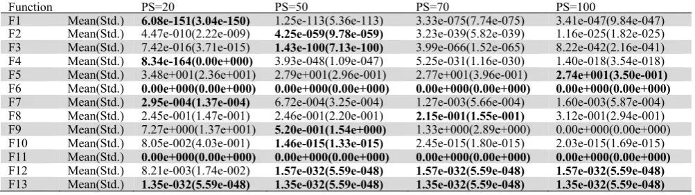
Table 1

Comparative statistical results of 13 benchmark function of E-BSADE for different values of population size (PS) at D=30 over 25 runs, after 200000 function evaluations.

Function PS=20 PS=50 PS=70 PS=100

F1 Mean(Std.) 6.08e-151(3.04e-150) 1.25e-113(5.36e-113) 3.33e-075(7.74e-075) 3.41e-047(9.84e-047)

F2 Mean(Std.) 4.47e-010(2.22e-009) 4.25e-059(9.78e-059) 3.23e-039(5.82e-039) 1.16e-025(1.82e-025)

F4 Mean(Std.) 8.34e-164(0.00e+000) 3.93e-048(1.09e-047) 5.25e-031(1.16e-030) 1.40e-018(3.54e-018)

F5 Mean(Std.) 3.48e+001(2.36e+001) 2.79e+001(2.96e-001) 2.77e+001(3.96e-001) 2.74e+001(3.50e-001)

F6 Mean(Std.) 0.00e+000(0.00e+000) 0.00e+000(0.00e+000) 0.00e+000(0.00e+000) 0.00e+000(0.00e+000)

F7 Mean(Std.) 2.95e-004(1.37e-004) 6.72e-004(3.25e-004) 1.27e-003(5.66e-004) 1.60e-003(5.87e-004)

F8 Mean(Std.) 2.45e-001(1.47e-001) 2.46e-001(2.20e-001) 2.15e-001(1.55e-001) 3.12e-001(2.94e-001)

F9 Mean(Std.) 7.27e+000(1.37e+001) 5.20e-001(1.54e+000) 1.33e+000(2.89e+000) 0.00e+000(0.00e+000)

F11 Mean(Std.) 0.00e+000(0.00e+000) 0.00e+000(0.00e+000) 0.00e+000(0.00e+000) 0.00e+000(0.00e+000)

F12 Mean(Std.) 8.21e-003(1.74e-002) 1.57e-032(5.59e-048) 1.57e-032(5.59e-048) 1.57e-032(5.59e-048)

(7)

The average time is also recorded. In this experiment VTR is chosen as 1e-8. Moreover, in the present work, the effect of the common controlling parameters of the algorithm i.e. population size and number of generations on the performance of the algorithm are also investigated by considering different population sizes and number of generations (function evaluation).

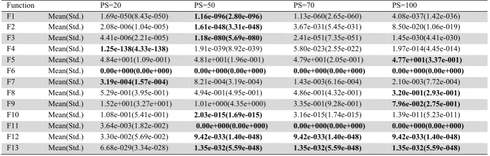
Table 2

Comparative statistical results of 13 benchmark function of E-BSADE for different values of population size (PS) at D=50, over 25 runs, after 200000 function evaluations.

F1 Mean(Std.) 1.69e-050(8.43e-050) 1.16e-096(2.80e-096) 1.13e-060(2.65e-060) 4.08e-037(1.42e-036) F2 Mean(Std.) 2.08e-006(1.04e-005) 1.61e-048(3.31e-048) 3.67e-031(5.45e-031) 8.50e-020(1.06e-019) F3 Mean(Std.) 4.41e-006(2.21e-005) 1.18e-080(5.69e-080) 2.41e-051(7.35e-051) 1.45e-030(4.41e-030) F4 Mean(Std.) 1.25e-138(4.33e-138) 1.91e-039(8.92e-039) 5.80e-023(2.55e-022) 1.97e-014(4.45e-014) F5 Mean(Std.) 4.84e+001(1.09e-001) 4.81e+001(1.96e-001) 4.79e+001(2.05e-001) 4.77e+001(3.37e-001)

F6 Mean(Std.) 0.00e+000(0.00e+000) 0.00e+000(0.00e+000) 0.00e+000(0.00e+000) 0.00e+000(0.00e+000)

F7 Mean(Std.) 3.19e-004(1.57e-004) 8.21e-004(3.19e-004) 1.43e-003(6.16e-004) 2.10e-003(7.72e-004) F8 Mean(Std.) 5.29e-001(3.95e-001) 4.94e-001(4.95e-001) 4.86e-001(4.32e-001) 3.20e-001(2.93e-001)

F9 Mean(Std.) 1.52e+001(3.27e+001) 1.01e+000(4.35e+000) 3.35e-001(9.28e-001) 7.96e-002(2.75e-001)

F10 Mean(Std.) 1.08e-001(5.41e-001) 2.03e-015(1.69e-015) 3.16e-015(1.74e-015) 1.39e-011(5.23e-011) F11 Mean(Std.) 3.64e-003(1.82e-002) 0.00e+000(0.00e+000) 0.00e+000(0.00e+000) 0.00e+000(0.00e+000)

F12 Mean(Std.) 3.30e-002(5.69e-002) 9.42e-033(1.40e-048) 9.42e-033(1.40e-048) 9.42e-033(1.40e-048)

F13 Mean(Std.) 6.68e-029(3.34e-028) 1.35e-032(5.59e-048) 1.35e-032(5.59e-048) 1.35e-032(5.59e-048)

Table 1 and 2 shows the effect of population size on the performance of the algorithm, the algorithm is experimented with different population sizes viz. 20, 50, 70 and 100 and dimension viz. 30 and 50 with function evaluations in each strategy is 200000 (for function F1 to F13). For the considered test problems, the E-DEBSA algorithm runs 25 times for each benchmark function. Boldface represents the best solution found after reaching the maximum number of function evaluations. From Table 1, it is observed that for functions F1, F4, and F7, strategy with population size of 20 and number of function evaluations 200000 produced the best results than the other strategies. For functions F2, F3, F9, and F10, strategy with population size of 50 gave the best results. For functions F8, strategy with population size of 70 and for functions F5, strategy with population size of 100 produced the best results. For functions F6, F11 and F13 strategies produced the same results and hence no effect of population size on these functions to achieve their respective global optimum values with same number of function evaluations. For function F12, strategy with population size 50, 70 and 100 produced the identical results. Similarly, it is observed from Table 2 that for functions F4 and F7 strategy with population size 20 produced best results than the other strategies. For functions F1, F2, F3, and F10, strategy with population size 50 produced best results than the other strategies. For functions F5, F8, and F9, strategy with population size 100 produced best results than the other strategies. For functions F6, strategies produced the same results and hence no effect of population size on these functions to achieve their respective global optimum values with same number of function evaluations. For function F11, F12, and F13 strategy with population size 50, 70 and 100 produced the identical results.

Table 3

Comparative statistical results of 8 benchmark function (F14-F21) of E-BSADE for different values of population size (PS) over 30 runs, after 10000 function evaluation.

F14 Mean(Std.) 3.34e-002(1.81e-001) 2.00e-010(7.36e-010) 2.98e-011(5.90e-011) 4.19e-011(8.93e-011) F15 Mean(Std.) 8.41e-004(8.40e-004) 9.77e-005(1.22e-004) 1.61e-004(1.19e-004) 1.98e-004(1.16e-004) F16 Mean(Std.) 1.15e-004(5.43e-004) 4.65e-008(1.12e-016) 4.65e-008(1.06e-016) 4.65e-008(2.52e-015) F17 Mean(Std.) 9.22e-005(4.65e-004) 7.36e-006(0.00e+000) 7.36e-006(0.00e+000) 7.36e-006(1.10e-012)

F18 Mean(Std.) 6.30e-002(3.45e-001) 0.00e+000(0.00e+000) 0.00e+000(0.00e+000) 0.00e+000(0.00e+000)

(8)

Table 3 also shows the effect of population size on the performance of the algorithm, the algorithm is experimented with different population sizes viz. 20, 50, 70 and 100 with function evaluations in each strategy 10000 (for function F14 to F21). For the considered test problems, the E-DEBSA algorithm runs 30 times for each benchmark function. It is observed from Table 3 that for functions F16, strategy with population size of 50 produced the best results than the other strategies. For functions F14, F15, F19, F20, and F21 strategy with population size of 70 produced the best results than the other strategies. For function F17, and F18 strategy with population size 50, 70 and 100 produced the identical results.

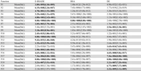
Table 4

Comparative statistical results of 21 benchmark function of E-BSADE with two other state-of-the-art algorithms

Function E-BSADE BSA DE

F1 Mean(Std.) 1.89e-095(6.10e-095) 1.40e-012(1.29e-012) 4.98e-032(1.42e-031)

F2 Mean(Std.) 6.15e-048(2.24e-047) 7.45e-008(4.77e-008) 1.77e-019(2.23e-019) F3 Mean(Std.) 4.70e-081(1.53e-080) 1.24e-011(9.48e-012) 3.28e-031(5.24e-031)

F4 Mean(Std.) 3.29e-040(1.31e-039) 5.67e+000(1.28e+000) 2.20e+001(4.86e+000) F5 Mean(Std.) 4.80e+001(2.42e-001) 9.10e+001(3.68e+001) 1.13e+002(1.62e+002)

F6 Mean(Std.) 0.00e+000(0.00e+000) 0.00e+000(0.00e+000) 2.68e+000(2.58e+000) F7 Mean(Std.) 1.05e-003(3.79e-004) 2.51e-002(6.65e-003) 1.76e-002(5.07e-003) F8 Mean(Std.) 3.44e-001(3.33e-001) 6.24e+001(1.07e+002) 2.54e-001(2.18e-001)

F9 Mean(Std.) 3.18e-001(8.96e-001) 1.03e+001(2.95e+000) 3.44e+001(8.49e+000)

F10 Mean(Std.) 2.45e-015(1.80e-015) 5.21e-007(7.66e-007) 1.22e-001(3.41e-001) F11 Mean(Std.) 0.00e+000(0.00e+000) 4.84e-012(1.90e-011) 4.04e-003(7.47e-003)

F12 Mean(Std.) 9.42e-033(1.40e-048) 4.24e-013(9.02e-013) 1.98e-002(5.68e-002) F13 Mean(Std.) 1.35e-032(5.59e-048) 9.59e-014(1.28e-013) 2.64e-003(9.13e-003)

F14 Mean(Std.) 2.23e-010(6.72e-010) 5.47e-009(1.20e-008) 1.63e-014(7.63e-014)

F15 Mean(Std.) 1.98e-004(1.68e-004) 7.06e-004(3.01e-004) 6.18e-004(1.90e-004) F16 Mean(Std.) 4.65e-008(1.12e-016) 5.01e-008(6.28e-009) 4.65e-008(9.06e-017)

F17 Mean(Std.) 7.36e-006(0.00e+000) 7.50e-006(2.64e-007) 7.36e-006(0.00e+000)

F18 Mean(Std.) 0.00e+000(0.00e+000) 2.61e-007(5.50e-007) 0.00e+000(0.00e+000)

F19 Mean(Std.) 3.21e-007(3.51e-010) 1.75e-001(3.08e-001) 3.21e-007(7.25e-016)

F20 Mean(Std.) 2.69e-001(1.34e+000) 1.17e-001(1.45e-001) 6.77e-009(7.17e-009)

F21 Mean(Std.) 2.14e-001(1.07e+000) 2.16e-001(3.78e-001) 2.22e-009(2.11e-009)

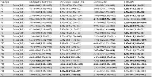
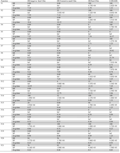
The comparative results of each benchmark function given in Appendix 1 are presented in Tables 4-7 in the form of best solution. For each algorithm and each test function, 25 independent runs were conducted with 200000 function evaluations (FES) for function (F1 to F13) and 10000 function evaluations (FES) for function (F14 to F21) as the termination criterion. The population size was set to 50. Table 4 shows the comparison result of the proposed algorithm with the basic DE and BSA; boldface represents the best solution found after reaching the maximum number of function evaluations. From this table it is seen that the proposed algorithm found better performance in most of the cases from the other two algorithms. Also it is observed that that the proposed algorithm found better performance except for function no F8, F14, F20 and F21. The successful runs (SR), successful performance (SP) and average time are recorded which are given in Table 5, compared to basic DE, BSA.

(9)

Table 5

Comparative SR, SP and Average time of 21 benchmark function with BSA and DE algorithms.

Function E-BSADE BSA DE Function E-BSADE BSA DE

F1 SR 100 100 100 F12 SR 96 100 76

SP 2.82E+04 1.49E+05 6.93E+04 SP 3.36E+04 1.40E+05 1.73E+05 Avg.time 1.33 13.65 2.54 Avg.time 7.29 15.09 9.97

F2 SR 100 0 100 F13 SR 100 100 88

SP 4.03E+04 Inf 9.73E+04 SP 2.58E+04 1.33E+05 1.06E+05 Avg.time 2.14 21.79 3.66 Avg.time 5.06 13.54 6.27

F3 SR 100 100 100 F14 SR 100 96 100

SP 3.51E+04 1.65E+05 7.60E+04 SP 1.84E+03 7.33E+03 2.87E+03 Avg.time 3.02 19.27 3.99 Avg.time 1.33 4.6 0.65

F4 SR 100 0 0 F15 SR 4 0 8

SP 5.78E+04 Inf Inf SP 2.49E+05 Inf 1.24E+05

Avg.time 3.27 16.49 7.55 Avg.time 1.25 1.02 0.45

F5 SR 0 0 0 F16 SR 0 0 0

SP Inf Inf Inf SP Inf Inf Inf

Avg.time 16.37 16.16 7.42 Avg.time 0.88 0.71 0.36

F6 SR 100 100 40 F17 SR 0 0 0

SP 1.27E+04 5.25E+04 3.34E+05 SP Inf Inf Inf Avg.time 1.23 4.43 5.1 Avg.time 0.84 0.65 0.35

F7 SR 0 0 0 F18 SR 100 60 100

SP Inf Inf Inf SP 2.72E+03 1.56E+04 2.38E+03

Avg.time 24.82 27.71 8.97 Avg.time 0.23 0.64 0.09

F8 SR 0 0 0 F19 SR 0 0 0

SP Inf Inf Inf SP Inf Inf Inf

Avg.time 21.79 20.35 8.53 Avg.time 1.23 1.05 0.48

F9 SR 84 0 0 F20 SR 84 0 84

SP 7.91E+04 Inf Inf SP 9.28E+03 Inf 8.64E+03

Avg.time 6.73 225.06 8.28 Avg.time 0.93 1.08 0.35

F10 SR 100 0 92 F21 SR 92 0 100

SP 7.97E+04 Inf 1.24E+05 SP 7.50E+03 Inf 5.52E+03 Avg.time 8.74 16.15 4.68 Avg.time 0.83 1.07 0.27

F11 SR 100 100 80

SP 3.03E+04 1.53E+05 1.20E+05 Avg.time 3.25 7.02 3.85

Table 6

Comparative statistical results of 21 benchmark function of E-BSADE with respect to other DE Mutation Strategies.

Function DE/target to best/1/bin DE/Current to rand/1/bin DE/best/2/bin E-BSADE F1 Mean(Std.) 6.60e+003(1.88e+003) 2.27e+000(4.12e+000) 1.93e-048(5.49e-048) 1.89e-095(6.10e-095)

F2 Mean(Std.) 4.51e+001(8.46e+000) 1.05e-002(2.90e-002) 2.03e-024(8.77e-024) 6.15e-048(2.24e-047)

F3 Mean(Std.) 1.52e+005(4.59e+004) 4.78e+001(9.20e+001) 1.09e-046(3.77e-046) 4.70e-081(1.53e-080)

F4 Mean(Std.) 2.16e+001(3.07e+000) 1.31e+001(3.55e+000) 1.95e+001(3.44e+000) 3.29e-040(1.31e-039)

F5 Mean(Std.) 2.06e+006(8.99e+005) 3.24e+002(4.30e+002) 4.12e+001(3.79e+001) 4.80e+001(2.42e-001) F6 Mean(Std.) 5.93e+003(1.01e+003) 1.92e+001(2.21e+001) 3.87e+001(2.72e+001) 0.00e+000(0.00e+000)

F7 Mean(Std.) 3.95e-001(2.59e-001) 1.24e-002(6.70e-003) 2.92e-002(1.22e-002) 1.05e-003(3.79e-004)

F8 Mean(Std.) 4.28e+001(2.14e+002) 2.95e-001(3.17e-001) 2.74e-001(2.61e-001) 3.44e-001(3.33e-001) F9 Mean(Std.) 1.38e+002(2.69e+001) 3.22e+002(1.53e+001) 1.96e+002(1.39e+002) 3.18e-001(8.96e-001)

F10 Mean(Std.) 1.16e+001(9.51e-001) 1.26e+000(6.09e-001) 2.82e+000(8.00e-001) 2.45e-015(1.80e-015)

F11 Mean(Std.) 6.33e+001(1.33e+001) 9.35e-002(1.13e-001) 1.75e-002(2.05e-002) 0.00e+000(0.00e+000)

F12 Mean(Std.) 2.40e+004(9.50e+004) 1.81e-001(2.26e-001) 6.49e-001(1.12e+000) 9.42e-033(1.40e-048)

F13 Mean(Std.) 7.65e+005(1.49e+006) 5.64e-002(1.20e-001) 4.32e+001(5.67e+001) 1.35e-032(5.59e-048)

F14 Mean(Std.) 4.08e-014(1.15e-013) 1.28e-007(4.43e-007) 2.47e-014(7.10e-014) 2.23e-010(6.72e-010) F15 Mean(Std.) 3.26e-004(3.99e-004) 5.37e-004(2.92e-004) 3.31e-004(4.12e-004) 1.98e-004(1.68e-004)

F16 Mean(Std.) 4.65e-008(1.09e-016) 4.65e-008(5.81e-014) 4.65e-008(1.02e-016) 4.65e-008(1.12e-016)

F17 Mean(Std.) 7.36e-006(0.00e+000) 7.51e-006(4.76e-007) 7.36e-006(0.00e+000) 7.36e-006(0.00e+000)

F18 Mean(Std.) 0.00e+000(0.00e+000) 0.00e+000(0.00e+000) 0.00e+000(0.00e+000) 0.00e+000(0.00e+000)

F19 Mean(Std.) 2.70e+000(3.68e+000) 2.08e-004(6.75e-004) 3.43e+000(2.98e+000) 3.21e-007(3.51e-010)

(10)

Table 7

Comparative SR, SP and Average time of 21 benchmark function with other DE mutation strategies.

Function DE/target to best/1/bin DE/Current to rand/1/bin DE/best/2/bin E-BSADE

F1 SR 0.00 0.00 100 100

SP Inf Inf 4.75E+04 2.82E+04

Avg.time 7.19 6.97 1.79 1.33

F2 SR 0.00 52 100 100

SP Inf 3.85E+05 7.32E+04 4.03E+04

Avg.time 7.39 7.14 2.8 2.14

F3 SR 0.00 0.00 100 100

SP Inf Inf 5.26E+04 3.51E+04

Avg.time 10.4 10.15 2.8 3.02

F4 SR 0.00 0.00 0 100

SP Inf Inf Inf 5.78E+04

Avg.time 7.44 7.15 7.63 3.27

F5 SR 0.00 0.00 0 0

SP Inf Inf Inf Inf

Avg.time 7.27 7.01 7.54 16.37

F6 SR 0.00 0.00 0 100

Avg.time 7.56 7.21 7.71 1.23

F7 SR 0.00 0.00 0 0

SP Inf Inf Inf Inf

Avg.time 8.87 8.54 9.05 24.82

F8 SR 0.00 0.00 0 0

SP Inf Inf Inf Inf

Avg.time 8.27 8.04 8.6 21.79

F9 SR 0.00 0.00 0 84

Avg.time 8.19 7.81 8.39 6.73

F10 SR 0.00 0.00 0 100

Avg.time 8.22 7.85 8.38 8.74

F11 SR 0.00 0.00 60 100

SP Inf Inf 1.81E+05 3.03E+04

Avg.time 8.03 7.65 4.42 3.25

F12 SR 0.00 4 32 96

SP Inf 5.00E+06 5.47E+05 3.36E+04

Avg.time 14.95 14.22 13.33 7.29

F13 SR 0.00 0.00 24 100

SP Inf Inf 7.72E+05 2.58E+04

Avg.time 13.3 12.79 12.51 5.06

F14 SR 100 52 100 100

SP 1.89E+03 1.92E+04 2.17E+03 1.84E+03

Avg.time 0.42 2.17 0.49 1.33

F15 SR 28 0.00 44 4

SP 2.92E+04 Inf 1.78E+04 2.49E+05

Avg.time 0.37 0.44 0.37 1.25

F16 SR 0.00 0.00 0 0

SP Inf Inf Inf Inf

Avg.time 0.36 0.34 0.36 0.88

F17 SR 0.00 0.00 0 0

SP Inf Inf Inf Inf

Avg.time 0.35 0.33 0.36 0.84

F18 SR 100 100 100 100

SP 1.73E+03 1.00E+04 1.89E+03 2.72E+03

Avg.time 0.06 0.35 0.07 0.23

F19 SR 0.00 0.00 0 0

SP Inf Inf Inf Inf

Avg.time 0.48 0.46 0.49 1.23

F20 SR 84 56 80 84

SP 5.77E+03 1.79E+04 7.96E+03 9.28E+03

Avg.time 0.23 0.46 0.31 0.93

F21 SR 76 92 64 92

SP 6.14E+03 1.09E+04 9.36E+03 7.50E+03

(11)

Table 8

Comparative statistical results of 13 benchmark function of E-BSADE with other state-of-the-art PSO variants.

Function Mean(Std.) FDR-PSO CPSO-H UPSO CLPSO E-BSADE F1 Mean(Std.) 4.90e-045(2.03e-044) 1.63e-004(1.14e-004) 9.64e-039(8.30e-039) 8.82e-007(3.26e-007) 6.71e-076(2.17e-075)

F2 Mean(Std.) 1.86e-015(8.24e-015) 3.28e-003(7.49e-004) 3.51e-023(2.31e-023) 9.69e-005(1.54e-005) 1.74e-038(3.79e-038)

F4 Mean(Std.) 6.22e-001(2.29e-001) 1.06e+001(3.55e+000) 3.02e-001(1.96e-001) 1.62e+001(1.21e+000) 1.40e-030(4.88e-030)

F5 Mean(Std.) 3.69e+001(3.03e+001) 3.99e+001(3.47e+001) 4.54e+001(2.70e+001) 8.84e+001(3.66e+001) 3.81e+001(1.45e-001) F6 Mean(Std.) 1.65e+000(1.39e+000) 0.00e+000(0.00e+000) 0.00e+000(0.00e+000) 0.00e+000(0.00e+000) 0.00e+000(0.00e+000)

F8 Mean(Std.) 3.67e+003(1.15e+003) 4.15e+001(6.95e+001) 2.62e-004(5.60e-004) 1.79e-002(1.26e-002) 5.45e-001(3.55e-001) F9 Mean(Std.) 5.26e+001(8.87e+000) 4.18e-005(2.64e-005) 9.02e+001(1.87e+001) 1.96e-001(1.30e-001) 1.52e-001(4.95e-001) F10 Mean(Std.) 4.41e-014(1.71e-014) 2.53e-003(6.31e-004) 7.64e-015(1.09e-015) 5.51e-004(1.06e-004) 2.31e-015(1.79e-015)

F11 Mean(Std.) 9.22e-003(1.34e-002) 1.30e-002(2.40e-002) 4.44e-017(1.99e-016) 1.66e-005(8.02e-006) 0.00e+000(0.00e+000)

F13 Mean(Std.) 2.75e-003(4.88e-003) 3.91e-006(4.80e-006) 1.35e-032(2.81e-048) 5.91e-007(1.04e-007) 1.35e-032(2.81e-048)

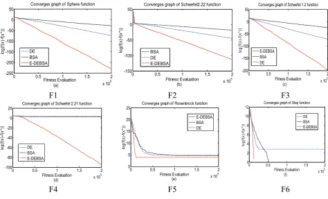
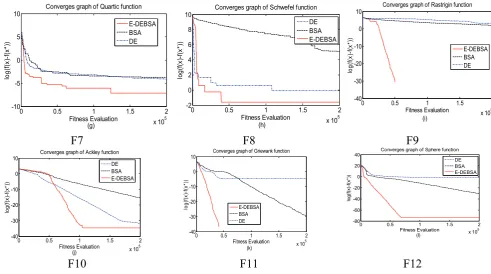
The performance of E-DEBSA is also compared with the different PSO variants like FDR-PSO (Peram et al., 2003), CPSO-H (Van den Bergh & Engelbrecht, 2004), UPSO (Parsopoulos & Vrahatis, 2004), and CLPSO (Liang et al., 2006) for the same number of function evaluations. The comparative results of each 13 benchmark function (F1 to F13) are presented in Tables 8 in the form of average solution and standard deviation obtained in 20 independent runs on each benchmark function with the population size is 50, dimension (D) is 40 and maximum number of function evaluation is 150000. The boldface value given in parenthesis indicates the global optimum value of that function. From Table 8 it is observed that the proposed method perform best solution except for function F5, F8 and F9. Also for F6 and F11, E-DEBSA reaches the global optimum solution. Fig. 1(a)-(l) shows the convergence graph of E-E-DEBSA. To be specific, we observe that the convergence curve of E-DEBSA in functions F1–F4 (Fig. 1(a)–(d)) linearly increased to the optimum point. For function F5, Fig.1.(e) the converges graph curvilinear increased to optimum point. Also for F6-F13, the converges graph Fig.1(f)-Fig.1.(l), the proposed method E-DEBSA converges faster to the global optimum.

F1 F2 F3

F4 F5 F6

0 0.5 1 1.5 2

x 105 -250 -200 -150 -100 -50 0 50 Fitness Evaluation log( f( x) -f (x *) )

Converges graph of Sphere function

DE BSA E-DEBSA

(a)

0 0.5 1 1.5 2

x 105 -150 -100 -50 0 50 Fitness Evaluation lo g( f( x)-f (x *) )

Converges graph of Schwefel2.22 function

BSA DE E-DEBSA

(b)

0 0.5 1 1.5 2 x 105 -200 -150 -100 -50 0 50 Fitness Evaluation lo g( f( x)-f (x *) )

Converges graph of Schwefel 1.2 function

E-DEBSA BSA DE

(c)

0 0.5 1 1.5 2 x 105 -100 -80 -60 -40 -20 0 20 Fitness Evaluation lo g( f( x) -f (x *) )

Converges graph of Schwefel 2.21 function

DE BSA E-DEBSA

(d)

0 0.5 1 1.5 2 x 105 0 5 10 15 20 25 Fitness Evaluation lo g( f(x )-f(x *) )

Converges graph of Rosenbrock function

E-DEBSA BSA DE

(e)

0 0.5 1 1.5 2 x 105 0 2 4 6 8 10 12 Fitness Evaluation lo g( f( x)-f(x *) )

Converges graph of Step function

DE BSA E-DEBSA

(12)

F7 F8 F9

F10 F11 F12

Fig. 1. Convergence curves of 50 dimensional test functions: (a) F1, (b) F2, (c) F3, (d) F4, (e) F5, (f) F6, (g) F7, (h) F8, (i) F9 , (j) F10 , (k) F11 , and (l) F12 .

5. Conclusions

Since the combination of two algorithms can provide a higher efficiency and flexibility when dealing with real-world and large scale problems, this paper proposed an ensemble algorithm of DE and BSA called E-DEBSA. For the validity of the proposed method, 21 different benchmark functions have been considered and the result has been compared to basic DE, BSA and different DE mutation strategies. Also the result are compared with different PSO variants. Moreover, the effect of common controlling parameters (i.e. population size, and number of generations) on the performance of E-DEBSA algorithm has also been investigated by considering different combinations of common controlling parameters. Also, in general, the strategy with higher population size has produced better results than that with smaller population size for same number of function evaluations for lower dimension and strategy with lower population size has produced better results than that with higher population size for same number of function evaluations for higher dimension. From the above experimental results and discussion it can be suggeste that its overall performance was better than the other competitors.

References

Behnamian, J., Zandieh, M., & Ghomi, S. F. (2009). Parallel-machine scheduling problems with

sequence-dependent setup times using an ACO, SA and VNS hybrid algorithm. Expert Systems with

Applications, 36(6), 9637-9644.

Blum, C. (2005). Ant colony optimization: Introduction and recent trends.Physics of Life reviews, 2(4),

353-373.

Civicioglu, P. (2013). Backtracking search optimization algorithm for numerical optimization

problems. Applied Mathematics and Computation, 219(15), 8121-8144.

Das, S. K. (2005). Slope stability analysis using genetic algorithm. The Electronic Journal of

Geotechnical Engineering, 10, 429-439.

0 0.5 1 1.5 2

x 105 -10

-5 0 5 10

Fitness Evaluation

lo

g(

f(

x)-f

(x

*)

)

Converges graph of Quartic function

E-DEBSA BSA DE

(g)

0 0.5 1 1.5 2

x 105 -2

0 2 4 6 8 10

Fitness Evaluation

lo

g(

f(

x)-f

(x

*)

)

Converges graph of Schwefel function DE BSA E-DEBSA

(h)

0 0.5 1 1.5 2

x 105 -40

-30 -20 -10 0 10

Fitness Evaluation

lo

g(

f(x

)-f(x

*)

)

Converges graph of Rastrigin function

E-DEBSA BSA DE

(i)

0 0.5 1 1.5 2 x 105 -40

-30 -20 -10 0 10

Fitness Evaluation

lo

g(

f(

x)-f

(x

*)

)

Converges graph of Ackley function DE BSA E-DEBSA

(j)

0 0.5 1 1.5 2 x 105 -40

-30 -20 -10 0 10

Fitness Evaluation

lo

g(

f(x

)-f

(x

*)

)

Converges graph of Griewank function

E-DEBSA BSA DE

(k)

0 0.5 1 1.5 2

x 105 -80

-60 -40 -20 0 20 40

Fitness Evaluation

lo

g(

f(

x)

-f

(x

*)

)

Converges graph of Sphere function

DE BSA E-DEBSA

(13)

Eskandar, H., Sadollah, A., Bahreininejad, A., & Hamdi, M. (2012). Water cycle algorithm–A novel metaheuristic optimization method for solving constrained engineering optimization

problems. Computers & Structures, 110, 151-166.

Fan, S. K. S., & Zahara, E. (2007). A hybrid simplex search and particle swarm optimization for

unconstrained optimization. European Journal of Operational Research, 181(2), 527-548.

Gämperle, R., Müller, S. D., & Koumoutsakos, P. (2002). A parameter study for differential

evolution. Advances in Intelligent Systems, Fuzzy Systems, Evolutionary Computation, 10, 293-298.

Glover, F., & Laguna, M. (1997). Tabu Search, Kluwer Academic Publishers, Norwell, MA.

Gong, W., Cai, Z., & Ling, C.X. (2010). DE/BBO: a hybrid differential evolution with biogeography-based optimization for global numerical optimization. Soft Computing, 15(4), 645–665.

Guo, W., Li, W., Zhang, Q., Wang, L., Wu, Q., & Ren, H. (2014). Biogeography-based particle swarm

optimization with fuzzy elitism and its applications to constrained engineering problems. Engineering

Optimization, 46(11), 1465-1484.

Zhang, J. R., Zhang, J., Lok, T. M., & Lyu, M. R. (2007). A hybrid particle swarm

optimization–back-propagation algorithm for feedforward neural network training. Applied Mathematics and

Computation, 185(2), 1026-1037.

Kennedy, J., & Eberhart, R.C. (1995). Particle swarm optimization, Proceedings of the 1995 IEEE International Conference on Neural Networks (Perth, Australia, IEEE Service Center, Piscataway, NJ, 1995), vol. 4, pp. 1942-1948.

Lampinen, J., & Zelinka, I. (2000). On stagnation of the differential evolution algorithm, in: Proceedings of MENDEL 2000, 6th International Mendel Conference on Soft Computing, pp. 76–83.

Lee, K. S., & Geem, Z. W. (2005). A new meta-heuristic algorithm for continuous engineering

optimization: harmony search theory and practice.Computer Methods in Applied Mechanics and

Engineering, 194(36), 3902-3933.

Liang, J. J., Qin, A. K., Suganthan, P. N., & Baskar, S. (2006). Comprehensive learning particle swarm

optimizer for global optimization of multimodal functions. Evolutionary Computation, IEEE

Transactions on, 10(3), 281-295.

Lin, W. Y. (2010). A GA–DE hybrid evolutionary algorithm for path synthesis of four-bar

linkage. Mechanism and Machine Theory, 45(8), 1096-1107.

Liu, H., Cai, Z., & Wang, Y. (2010). Hybridizing particle swarm optimization with differential evolution

for constrained numerical and engineering optimization.Applied Soft Computing, 10(2), 629-640.

Kao, Y. T., & Zahara, E. (2008). A hybrid genetic algorithm and particle swarm optimization for

multimodal functions. Applied Soft Computing, 8(2), 849-857.

Mallipeddi, R., Suganthan, P. N., Pan, Q. K., & Tasgetiren, M. F. (2011). Differential evolution algorithm

with ensemble of parameters and mutation strategies. Applied Soft Computing, 11(2), 1679-1696.

Nama, S., Saha, A. K., & Ghosh, S. (2015). Parameters Optimization of Geotechnical Problem Using Different Optimization Algorithm, vol-33, Geotechnical and Geological Engineering, DOI 10.1007/s10706-015-9898-0

Nourelfath, M., Nahas, N., & Montreuil, B. (2007). Coupling ant colony optimization and the extended

great deluge algorithm for the discrete facility layout problem. Engineering Optimization, 39(8),

953-968.

Parouha, R. P., Das, K. N., (2015), An efficient hybrid technique for numerical optimization and applications, Computers & Industrial Engineering, 83, 193–216.

Parsopoulos, K. E., & Vrahatis, M. N. (2004). UPSO: A unified particle swarm optimization

scheme. Lecture Series on Computer and Computational Sciences,1, 868-873.

Peram, T., Veeramachaneni, K., & Mohan, C. K. (2003, April). Fitness-distance-ratio based particle

swarm optimization. In Swarm Intelligence Symposium, 2003. SIS'03. Proceedings of the 2003

IEEE (pp. 174-181). IEEE.

Rahnamayan, S., Tizhoosh, H. R., & Salama, M. (2008). Opposition-based differential

(14)

Rao, R.V., & Savsani, V.J. (2012). Mechanical Design Optimization using Advanced Optimization Technique, Springer Series in Advanced Manufacturing, Springer, London, Heidelberg.

Ronkkonen, J., Kukkonen, S., & Price, K. V. (2005, September). Real-parameter optimization with

differential evolution. In Proc. IEEE CEC (Vol. 1, pp. 506-513).

Sadollah, A., Bahreininejad, A., Eskandar, H., & Hamdi, M. (2013). Mine blast algorithm: A new

population based algorithm for solving constrained engineering optimization problems. Applied Soft

Computing, 13(5), 2592-2612.

Sengupta, A., & Upadhyay, A. (2009). Locating the critical failure surface in a slope stability analysis

by genetic algorithm. Applied Soft Computing, 9(1), 387-392.

Shojaeefard, M. H., Khalkhali, A., Akbari, M., & Tahani, M. (2013). Application of Taguchi

optimization technique in determining aluminum to brass friction stir welding parameters. Materials

& Design, 52, 587-592.

Šmuc, T. (2002). Improving convergence properties of the differential evolution algorithm. Matoušek

and Ošmera [529], 80-86.

Storn, R.(1996). On the usage of differential evolution for function optimization, in: Biennial Conference of the North American Fuzzy Information Processing Society (NAFIPS), IEEE, Berkeley, pp. 519– 523.

Storn, R., & Price, K. (1995). Differential evolution-a simple and efficient adaptive scheme for global

optimization over continuous spaces (Vol. 3). Berkeley: ICSI.

Storn, R., & Price, K. (1997). Differential evolution–a simple and efficient heuristic for global

optimization over continuous spaces. Journal of Global Optimization, 11(4), 341-359.

Suganthan, P. N., Hansen, N., Liang, J. J., Deb, K., Chen, Y. P., Auger, A., & Tiwari, S. (2005). Problem definitions and evaluation criteria for the CEC 2005 special session on real-parameter

optimization. KanGAL report, 2005005.

Tizhoosh, H.R. (2005). Opposition-based learning: a new scheme for machine intelligence. International conference on computational intelligence for modelling control and automation; Austria. p. 695–701.

Van den Bergh, F., & Engelbrecht, A. P. (2004). A cooperative approach to particle swarm

optimization. Evolutionary Computation, IEEE Transactions on,8(3), 225-239.

Zaharie, D. (2009). Influence of crossover on the behavior of differential evolution algorithms. Applied

Soft Computing, 9(3), 1126-1138.

Zolfaghari, A. R., Heath, A. C., & McCombie, P. F. (2005). Simple genetic algorithm search for critical

non-circular failure surface in slope stability analysis. Computers and Geotechnics, 32(3), 139-152.

Rao, R., & Patel, V. (2013). Comparative performance of an elitist teaching-learning-based optimization

algorithm for solving unconstrained optimization problems. International Journal of Industrial

Engineering Computations, 4(1), 29-50.

Rao, R., & Patel, V. (2012). An elitist teaching-learning-based optimization algorithm for solving

complex constrained optimization problems. International Journal of Industrial Engineering

Computations, 3(4), 535-560.

Rao, R. V., Savsani, V. J., & Vakharia, D. P. (2011). Teaching–learning-based optimization: a novel

method for constrained mechanical design optimization problems. Computer-Aided Design, 43(3),

(15)

Appendix-1

F Function Formulation D Search

Space fmin 1 Sphere



  D i i x x f 1 2 )

( 50 [-100,100] 0

2 Schwefel2.

22





    D i D i i i x x x f 1 1 )

( 50 [-10,10] 0

3 Schwefel1.

2



   D i i j i x x f 1 1 2 )

( 50 [-100,100] 0

4 Schwefel2.

21 f(x)max



xi,1i D



50 [-100,100] 0

5 Rosenbrock



      D

i i i i

x x x x f 1 2 2 2

1 ) ( 1) ]

( 100 [ )

( 50 [-30, 30] 0

6 Step



   D i i x x f 1 2 ) 5 . 0 ( )

( 50 [-100,100] 0

7 Quartic



   D i i random ix x f 1 4 ) 1 , 0 ( )

( 50 [-1.28,1.28] 0

8 Schwefel





 sin( )

)

(x xi xi

f 50 [-500,500] -418.9828872724338*

D 9 Rastrigin



    D i i i x x D x f 1 2 )] 2 cos( 10 [ 10 )

(  50 [-5.12,5.12] 0

10 Ackley ) ) 2 cos( ( 1 ) 1 ( 1 1 2 20 20 ) (       i D i

i _D x

x D D e e e x f 

50 [-32,32] 0

11 Griewank 1 ) cos( 4000 ) ( 1 1 2   





  D i i D i i i x x x

f 50 [-600, 600] 0

12 Penalized1



               D i i D D i i i x u y y y D x f 1 2 1 1 2 2 2 ) 4 , 100 , 10 , ( ] ) 1 ( sin 10 1 [ ) 1 ( ) ( sin 10 ) (  

Where ( 1)

4 1

1 

 i i x y ,               a x a x a a x a x k a x k m k a x u i i i m i m i i ) ( 0 ) ( ) , , , (

50 [-50, 50] 0

13 Penalized2



                D i i D D D i i i x u x x x x x f 1 2 2 1 1 2 2 2 ) 4 , 100 , 5 , ( )]] 2 ( sin 1 [ ) 1 ( sin 10 1 [ ) 1 ( ) ( sin 10 1 . 0 ) ( 

(16)

14 Foxholes 1 25 1 2 1 ] ) ( 1 500 1 [ ) (   



    j i ij i a x j x

f 2 [-65.536,65.5

36]

0.998004

15 Kowalik 2

11

1 2 ₃ ₄

2 2

1( )_]

[ ) (



     

i _i _i

i i i x x b b x b b x a x f

4 [-5,5] 0.0003075

16 Six Hump

Camel back 2

2 2 2 1 6 1 4 1 2

1 4 4

3 1 1 . 2 4 )

(x x x x x x x x

f       2 [-5,5] -1.0316285

17 Branin ) 8 1 1 ( 10 ) 6 5 4 1 . 5 ( ) ( 2 1 2 1 2 2

2     

 x x x

x f

 



2 [-5,10] and

[0,15] 0.398

18 Goldstein and Price )] 27 36 48 12 18 )( 3 2 ( 30 [ )] 3 6 14 3 14 10 ( ) 1 ( 1 [ ) ( 2 2 2 1 2 2 1 2 2 1 2 2 2 1 2 2 1 1 2 2 1 x x x x x x x x x x x x x x x x f                