www.atmos-meas-tech.net/5/2095/2012/ doi:10.5194/amt-5-2095-2012
© Author(s) 2012. CC Attribution 3.0 License.
Measurement
Techniques
Using sonic anemometer temperature to measure sensible heat flux
in strong winds
S. P. Burns1,3, T. W. Horst1, L. Jacobsen2, P. D. Blanken3, and R. K. Monson4 1National Center for Atmospheric Research, Boulder, Colorado, USA
2Campbell Scientific, Inc., Logan, Utah, USA
3Department of Geography, University of Colorado, Boulder, USA
4School of Natural Resources and the Environment, University of Arizona, Tucson, USA Correspondence to: S. P. Burns (sean@ucar.edu)
Received: 2 December 2011 – Published in Atmos. Meas. Tech. Discuss.: 12 January 2012 Revised: 16 August 2012 – Accepted: 16 August 2012 – Published: 3 September 2012
Abstract. Sonic anemometers simultaneously measure the
turbulent fluctuations of vertical wind (w0) and sonic temper-ature (Ts0), and are commonly used to measure sensible heat flux (H). Our study examines 30-min heat fluxes measured with a Campbell Scientific CSAT3 sonic anemometer above a subalpine forest. We comparedH calculated withTs toH
calculated with a co-located thermocouple and found that, for horizontal wind speed (U) less than 8 m s−1, the agree-ment was around±30 W m−2. However, forU >≈8 m s−1, the CSATH had a generally positive deviation fromH cal-culated with the thermocouple, reaching a maximum differ-ence of ≈250 W m−2 at U≈18 m s−1. With version 4 of
the CSAT firmware, we found significant underestimation of the speed of sound and thusTs in high winds (due to a
delayed detection of the sonic pulse), which resulted in the large CSAT heat flux errors. Although thisTserror is
qualita-tively similar to the well-known fundamental correction for the crosswind component, it is quantitatively different and directly related to the firmware estimation of the pulse ar-rival time. For a CSAT running version 3 of the firmware, there does not appear to be a significant underestimation of Ts; however, aTserror similar to that of version 4 may occur
if the CSAT is sufficiently out of calibration. An empirical correction to the CSAT heat flux that is consistent with our conceptual understanding of theTserror is presented. Within
a broader context, the surface energy balance is used to eval-uate the heat flux measurements, and the usefulness of side-by-side instrument comparisons is discussed.
1 Introduction
high-frequency response or averaging periods that are too short (Leuning et al., 2012).
Previous studies have shown that sonic anemometers re-sult in erroneous sensible heat flux measurements during high winds (Grelle and Lindroth, 1996; Aubinet et al., 2000; Smedman et al., 2007). Grelle and Lindroth (1996) used a Gill Solent R2 and concluded that strong winds caused de-formation of the supports holding the sonic transducers and resulted in high-frequency noise that made an accurate heat flux measurement impossible. As an alternative, they calcu-latedHusing a co-located fast-response 0.025 mm platinum wire resistance thermometer (PRT). The study by Smedman et al. (2007) used two co-located Gill Solent models R2 and R3 sonic anemometers and found that, independent of stability conditions, sonic-measured heat flux had a larger magnitude than H with an alternative temperature sensor. Grelle and Lindroth (1996) also tested three other models of sonic anemometers and found similar problems for wind speeds faster than 10 m s−1. Recent heat flux comparisons between a Solent R3 and an independent 0.1 mm diameter PRT have shown good agreement (e.g., Grelle and Burba, 2007), though we should note that the Grelle and Burba mea-surements were at a height of only 4 m and might not have experienced strong winds. Another issue with using sonic anemometers in cold, windy places is that blowing snow can drift between the sonic transducers which causes spikes in the sonic temperature (Foken, 1998) and results in an over-estimation of heat flux as well as misleading flux directions depending on whether the snow particle is moving upward or downward in the the path (L¨uers and Bareiss, 2011).
This paper uses a Campbell Scientific CSAT3 sonic anemometer (hereafter “CSAT”; Campbell Scientific, Inc., 2010) at the Niwot Ridge Subalpine Forest AmeriFlux site (NWT) to examine the sensible heat flux in strong winds. Turnipseed et al. (2002) studied the energy balance at the NWT site and found that, during the daytime, the sum of the turbulent fluxes equals 80–90 % of the radiative energy input into the forest. At night, under moderately turbulent conditions, the energy balance closure is comparable to the daytime. However, when the nighttime conditions are ei-ther calm or extremely turbulent, the sensible and latent heat fluxes only equal 20–60 % of the net longwave radiative flux. Turnipseed et al. (2002) discussed several possible reasons for this nighttime discrepancy (e.g., instrument error, foot-print mismatch, horizontal advection), but none of these rea-sons could adequately explain the fact that the nighttime im-balance existed in the presence of strong winds. They con-cluded that the sonic temperature did not have sufficient res-olution to capture the small temperature fluctuations, which led to inaccurate sensible heat fluxes.
In early 2008 the sonic anemometers at NWT were re-calibrated (details in Sect. 2.3). After the recalibration, the new sensible heat flux still did not improve the agreement between the daytime and nocturnal energy balance in windy conditions, and the imbalance was even more dramatic than
before the recalibration. The goals of the current study are to (1) describe the discrepancy observed in the calculated sensi-ble heat flux, (2) compare the heat flux calculated using sonic temperature to that calculated with a co-located thermocou-ple, (3) present independent wind-tunnel results that attempt to explain the tower observations, (4) briefly describe Camp-bell Scientific, Inc. testing of the CSAT, (5) present a con-ceptual model of the CSAT error and suggest an empirical correction method to the CSAT heat flux, and (6) re-visit the surface energy balance results from Turnipseed et al. (2002) in light of the results from items (1)–(5).
2 Data and methods
2.1 Site description
This study uses data from the Niwot Ridge Subalpine For-est AmeriFlux site which is located below Niwot Ridge, Colorado, 8 km east of the Continental Divide (40◦105800N, 105◦3204700W, 3050 m elevation). The NWT measurements
started in November 1998 as described in Monson et al. (2002) and Turnipseed et al. (2002, 2003). The tree den-sity around the NWT Tower is≈0.4 trees m−2 with a leaf area index (LAI) of 3.8–4.2 m2m−2and tree heights of 12– 13 m (Turnipseed et al., 2002). In winter, NWT is a dry and windy place. Between November–February, the 30-min av-erage 21.5 m wind speed (U) is around 7 m s−1(standard de-viation≈4.5 m s−1) with a maximum near 20 m s−1. Typi-cal wintertime mid-day sensible heat flux values are on the order of 200 W m−2, while latent heat flux is usually less than 40 W m−2(Turnipseed et al., 2002). On top of Niwot Ridge (i.e., above tree-line), blowing snow is common (Berg, 1986) and snow/ice particles are often blown downslope over the forest. More information on NWT is available on-line at http://public.ornl.gov/ameriflux/.
2.2 Sonic anemometer thermometry
A few of the important relationships related to sonic anemometer thermometry are summarized here; a more com-plete description of the technology is readily available (e.g., Kaimal and Businger, 1963; Schotanus et al., 1983; Kaimal and Gaynor, 1991; Foken, 2008b, and many others).
The relationship between air temperature (T), the speed of sound (c), and specific humidity (q) within the atmosphere is well-known:
T = c
2
γdRd
1
1+0.51q
, (1)
whereγd=cpa/cva= 1.4 is the dry air specific heat ratio,cpa
andcva are the dry air specific heat at constant pressure and
volume (J kg−1K−1), andRdis the gas constant for dry air
(287 J kg−1K−1).
by a path-length distance (d). The speed of sound is deter-mined from the measured times to transitd (t1in one
direc-tion andt2in the opposite direction) and the geometry of the
sound rays, such that 1
t1
+ 1 t2
= 2ccos(α)
d =
2 d
q
c2−V2
n, (2)
whereVn is the wind component perpendicular tod (i.e.,
cross-wind) and α= sin−1(Vn/c) is the deflection angle of
the sound ray off the transducer-path axis. Solving Eq. (2) forcand substituting it into Eq. (1) withq= 0, it follows that sonic temperature (Ts) is
Ts ≡
c2 γdRd
= 1 γdRd
"
d
2
21
t1
+ 1 t2
2
+Vn2
#
. (3)
In a moist atmosphere, air temperature is calculated fromTs
as
Tsair= Ts
1+0.51q. (4)
To determine the sonic-derived sensible heat fluxH, we as-sume(Tsair)0=T0, multiply each side of Eq. (4) by the vertical wind componentw, decompose the measured variables into mean and fluctuating components (i.e.,Ts=Ts+Ts0, etc.), and
perform Reynolds averaging. Neglecting higher-order terms (e.g., Fuehrer and Friehe, 2002) leads to
H ρ cp
=w0T0= "
w0 Tuc s
0
+2T u c2 u
0w0−0.51T w0q0 #
=hw0T0
s −0.51T w0q0 i
, (5)
where ρ is the air density (kg m−3), c
p is the specific
heat of moist air at constant pressure, and u is the hor-izontal wind component in streamwise coordinates (note thatρ=ρa+ρvandcp= ρacpa+ρvcpv/ρwhere the
sub-scripts “a” and “v” refer to dry air and water vapor, re-spectively). Tsuc is Ts without the cross-wind correction
(i.e., Tsuc=Ts−Vn2(γdRd)−1). The u0w0 term is the
so-called cross-wind correction term, but most modern sonic anemometers take this into account with internal processing software that corrects each individualTs sample for
cross-wind effects using Eq. (3) (Hignett, 1992). The implemen-tation of Eq. (3) varies depending on the sonic anemome-ter manufacturer, model, and signal-processing firmware (Loescher et al., 2005; Campbell Scientific, Inc., 2010).
2.3 Energy balance equation and instrumentation
If we neglect the vertical advection of heat, the terms in the surface energy balance are
Ra =Rnet−Gz−Ssoil−Scanopy=H+LE+Hadv, (6)
where Ra is the available energy. At NWT, net radiation
(Rnet) was measured atz≈25 m above the ground with both
a net (Radiation and Energy Balance Systems REBS, model Q*7.1) and a four-component (Kipp and Zonen, model CNR1) radiometer. The heat flux at the soil surface (G) is determined from the soil heat flux (Gz) measured at depthz
and the heat stored in the overlying soil layer (Ssoil). Canopy
storage (Scanopy) accounts for heat stored in the biomass
be-tween the ground and sensible heat flux measurement level. ScanopyandSsoilare typically less than 10 % ofRnet(Oncley
et al., 2007). At NWT,Gz was measured with multiple soil
heat flux plates (REBS, model HFT-1) at a depth of 10 cm, and Turnipseed et al. (2002) showed that the storage terms andGz were small (less than 8 % of Rnet). Therefore, we
neglectScanopyandSsoil and assume the surface heat flux is
close to our measured soil heat flux (i.e.,G≈Gz). The
hori-zontal advection of heat (Hadv) requires spatially distributed
measurements, and is thought to be a primary reason that Eq. (6) does not balance at most flux sites (Leuning et al., 2012). In our discussions, the simple SEB closure fraction will be designated as CF (e.g., Barr et al., 2006) and refers to the ratio of the sum of the turbulent fluxes to (Rnet−G),
i.e., CF≡(H+ LE)/(Rnet−G). Similarly to Turnipseed et al.
(2002), we find nocturnal CF withRnetfrom the Q*7.1
sen-sor is about 15 % closer to closing the SEB than with the CNR1 sensor (see Burns et al., 2012 for details). For sim-plicity, only results with the Q*7.1Rnetsensor are presented
here.
Latent and sensible heat flux were measured atz≈21.5 m with a CSAT providing the high-frequency vertical wind (w0) and temperature (Ts0) fluctuations, while water vapor (q0) was measured with a co-located krypton hygrometer (Turnipseed et al., 2002). The 21.5 m CSAT was oriented so the along-sonic axis was pointed 203◦ from true north. Strong winds
at NWT are almost exclusively from the west (e.g., Burns et al., 2011) so that the angle between the wind vector and CSAT axis was≈67◦, well within the CSAT±170◦ accep-tance angle and also avoiding influence of the tower struc-ture (Friebel et al., 2009). Winds are rotated from sonic to planar-fit streamwise coordinates prior to the flux calcula-tions (Wilczak et al., 2001).Ts output by a CSAT is an
aver-age from the three non-orthogonal paths. We use “HCSAT” to
designate the heat flux calculated withTsfollowing Eq. (5).
The CSAT operates with either embedded-code firmware version 3 or version 4 (hereafter, ver3 and ver4) and uses ad-vanced digital signal processing to determine the ultrasonic times of flight (i.e.,t1 andt2 in Eq. 3). Ver4 is designed to
produce usable results when the signal is weak such as when liquid water is on the transducers, but degrades theTs
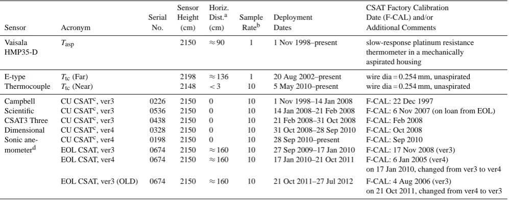
Table 1. A summary of NWT AmeriFlux tower temperature measurements used in our study.
Sensor Horiz. CSAT Factory Calibration
Serial Height Dist.a Sample Deployment Date (F-CAL) and/or
Sensor Acronym No. (cm) (cm) Rateb Dates Additional Comments
Vaisala Tasp 2150 ≈90 1 1 Nov 1998–present slow-response platinum resistance
HMP35-D thermometer in a mechanically
aspirated housing
E-type Ttc(Far) 2198 ≈136 1 20 Aug 2002–present wire dia = 0.254 mm, unaspirated
Thermocouple Ttc(Near) 2148 <3 10 5 May 2010–present wire dia = 0.254 mm, unaspirated
Campbell CU CSATc, ver3 0226 2150 0 10 1 Nov 1998–14 Jan 2008 F-CAL: 22 Dec 1997
Scientific CU CSATc, ver3 0536 2150 0 10 14 Jan 2008–21 Feb 2008 F-CAL: 6 Nov 2007 (on loan from EOL) CSAT3 Three CU CSATc, ver3 0438 2150 0 10 21 Feb 2008–31 Oct 2008 F-CAL: Feb 2008
Dimensional CU CSATc, ver4 0328 2150 0 10 31 Oct 2008–28 Sep 2010 F-CAL: Oct 2008
Sonic ane- CU CSATc, ver4 0198 2150 0 10 28 Sep 2010–present F-CAL: Sep 2010
mometerd EOL CSAT, ver3 0674 2150 ≈160 10 27 Sep 2009–17 Jan 2010 F-CAL: 17 Nov 2008 (ver3) EOL CSAT, ver4 0674 2150 ≈160 10 17 Jan 2010–21 Oct 2011 F-CAL: 6 Jan 2005 (ver4)
on 17 Jan 2010, changed from ver3 to ver4
EOL CSAT, ver3 (OLD) 0674 2150 ≈160 10 21 Oct 2011–27 Jul 2012 F-CAL: 4 Aug 2006 (ver3)
on 21 Oct 2011, changed from ver4 to ver3
aHorizontal distance from the University of Colorado (CU) CSAT sensor.bNumber of samples per second (Hz).cThe 2150 cm CU CSAT is used to determine the horizontal wind
speed (U).dThe CSAT sonic temperature (Ts) corrected for humidity isTsair=Ts(1 + 0.51q)−1whereqis specific humidity. The designation “ver3” and “ver4” represent CSAT
embedded code firmware versions 3 and 4, respectively. The CU and EOL CSATs are both mounted on booms that are oriented at 203◦from true north (e.g., pointed toward the southwest).
data were rarely flagged, however, for higher winds, around 2–4 % of the samples were flagged. The number of spikes was also affected by the relative humidity. Further details of the despiking can be found in the on-line discussion of Burns et al. (2012). Any CSAT data sample deemed questionable by the CSAT diagnostic flag was replaced with a linear fit between valid samples.
Here, we briefly summarize the sequence of events that led to our study (also see Table 1). In 2008, the three Univer-sity of Colorado (CU) CSATs (all ver3) were sent to Camp-bell Scientific, Inc. for recalibration and one of them (se-rial number 0328) was upgraded to ver4. After deploying CU CSAT 0328 at 21.5 m, we observed nighttimeHCSAT
val-ues that were frequently above zero, suggesting heat was be-ing transported from the surface to the atmosphere. Though such conditions are possible for short periods (e.g., due to warm air advection), we have rarely observed such phenom-ena in the previous 10 yr of measurements. These anoma-lousHCSATmeasurements were strongly correlated with high
winds (Fig. 1).
Because we were suspicious about these above-zero night-timeHCSATvalues, we deployed CSAT 0674 from the
Na-tional Center for Atmospheric Research (NCAR) Earth Ob-serving Laboratory (EOL) at the same level and orientation as the CU CSAT. The EOL CSAT 0674 initially used ver3, which we changed to ver4 partway through our study (Ta-ble 1). To change from ver3 to ver4, the processing chip in the CSAT electronics enclosure and the firmware version-specific calibration coefficients were both changed, but the sonic head was not disturbed.
40 41 42 43 44 45 46 47
−200 0 200 400 600
H
[W
m
−
2]
(a)
CU CSAT 0328, ver4
EOL CSAT 0674, ver4
T tc (Far)
40 41 42 43 44 45 46 47
0 5 10 15
Day of Year 2010, MST
U
[m
s
−
1]
(b)
Fig. 1. Time series of 21.5 m (a) sensible heat fluxH and (b) hor-izontal wind speedU.H is calculated using temperature from ei-ther a sonic anemometer or the far ei-thermocoupleTtcas specified in the legend (see Table 1 for details). The thermocouple uses the CU CSAT vertical wind to determineH.
Additional air temperature information was provided near the 21.5 m level by a 0.254 mm E-type thermocouple that was located about 1.4 m from the CU CSAT and sampled at 1 Hz. The thermocouple temperature fluctuations (Ttc0) are corre-lated withw0from the CU CSAT to calculate a sensible heat flux (e.g., HTtc=ρ cpw
0T0
tc). Because we were concerned
deployed in May 2010 within 3 cm of the CU CSAT trans-ducers and sampled at 10 Hz. These two thermocouples and their associated heat fluxes will be distinguished from each other using the terms “Near” and “Far” as shown in Ta-ble 1. The thermocouples used in our study were created by spot-welding the 0.254 mm chromel and constantan wires together and leaving the clipped ends intact to improve the thermal frequency-response (Fuehrer et al., 1994). The other temperature sensor at the 21.5 m level was a mechanically as-pirated, slow-response temperature-humidity sensor (Vaisala HMP35-D probe) which we use as a reference sensor for time-averaged comparisons.
3 Results and discussion
3.1 Comparison of sensible heat fluxes
If sensible heat flux is calculated using sonic temperature from two different CSATs and temperature from a co-located thermocouple, there are largeH differences during periods of strong winds that are most obvious at night (Fig. 1). In a perfect sonic anemometer, the path-lengthd is constant; however, real world changes to d can occur as the sensor material expands and contracts due to temperature changes or wind-induced stresses or vibrations (Smedman et al., 2007). Lanzinger and Langmack (2005) use a Thies two-dimensional sonic anemometer to show that a 50 K tempera-ture change results in a 0.4 mm change ind, which produces a 1.2 K error in Ts. We did not observe any
temperature-dependent heat flux differences in our study.
After separating the heat flux data by day and night, there is a consistent trend in theHCSAT−HTtc difference;
forU >≈8 m s−1,HCSAT−HTtc>0 and the difference
in-creases as wind speed inin-creases up to a difference of ≈250 W m−2atU≈17 m s−1 (Fig. 2). Our original obser-vation that this was primarily a nighttime problem is incor-rect, because the daytime and nighttime differences are qual-itatively similar. We have separated the panels of Fig. 2 into periods when different configurations of CSATs were on the tower (Table 1). By comparing Fig. 2a and b, we find that HCSAT EOL ver3 agreed better withHTtc thanHCSATEOL
ver4. Also,HCSAT−HTtc for EOL CSAT ver3 did not have
as strong a dependence on wind speed as ver4.
One issue of concern with the far thermocouple is the ≈1.4 m horizontal sensor separation from the CU CSAT (Horst and Lenschow, 2009). ForHCSAT−HTtc using either
the far (Fig. 2c) or near (Fig. 2d) thermocouple, a very sim-ilar pattern of increasingH difference with increasing wind speed is observed, implying that HTtc (Far)≈HTtc (Near).
This encourages us to believe that using the far thermocou-ple results in a viable heat flux. As one would expect, there is less scatter inHCSAT−HTtc using the near thermocouple.
The effect of sensor separation onHTtc (Far) and frequency
response of the thermocouples are revisited in Sect. 3.2.
In order to make a connection to the results from Turnipseed et al. (2002), we examined heat flux data col-lected within the period of 1998 to 2007. We found that HCSAT−HTtc(Far) using CSAT 0226 ver3 in 2007 has a
sim-ilar wind speed-dependence to that observed with the other CSATs (Fig. 2e). CSAT 0226 was initially deployed in 1998 (Table 1) which is relevant to our consideration of the surface energy balance in Sect. 3.6.
Although the focus here has been on the vertical heat flux, there are also differences in the horizontal heat flux (results not shown). We found that the ρ cp(u0Ts0−u0Ttc0)
difference is larger in magnitude and of opposite sign than theHCSAT−HTtc difference (i.e.,u0Ts0< u0Ttc0 whereas
w0T0 s> w0T
0
tc). We will provide further explanation for these
differences in Sect. 3.5.
The heat flux differences we have presented here are qual-itatively different from previous results using a Gill Solent sonic anemometer mentioned in the introduction (e.g., Grelle and Lindroth, 1996; Aubinet et al., 2000; Smedman et al., 2007). We foundHCSATtended to be larger thanHTtcas wind
speed increased for all conditions, whereas the Solent heat flux tended to be larger in magnitude thanH from the PRT. Therefore, in weakly stable conditions, we findHCSAT> HTtc
while the previous studies with the Gill sonic anemome-ter found HSolent< HPRT. In weakly unstable conditions,
HCSAT> HTtc andHSolent> HPRT. We would not necessarily
expect the two sonic anemometers to behave similarly (be-cause the CSAT and Solent have very different geometries, firmware, etc.), but it is worthwhile to note that the heat flux errors are in the opposite direction for weakly stable condi-tions, suggesting different reasons for the error.
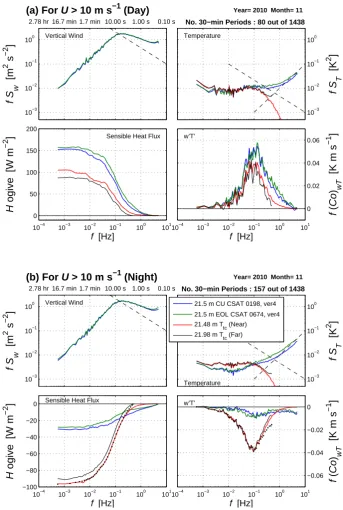
3.2 Spectral comparisons
To gain further insight into the HCSAT−HTtc differences,
we examine the spectra ofw0,Ts0, andTtc0 and their associ-ated cospectra and ogives (Friehe et al., 1991) for high-wind conditions (Fig. 3). The vertical wind and sonic temperature spectra from the two CSATs are in good agreement, but show the effect of high-frequency noise and aliasing. Forf >1 Hz, thef STs noise appears to follow thef
+1slope that is typical
of white noise, and indicative of the true temperature sig-nal dropping below the sensor noise threshold (Kaimal and Gaynor, 1991; Kaimal and Finnigan, 1994). Low-pass fil-teringTs to remove this noise did not significantly change
HCSAT(Burns et al., 2012). The temperature spectra from the
thermocouples are attenuated at frequencies above≈1 Hz, because the thermal mass of the thermocouple wire limits the response time. In high-wind conditions (i.e., when the f Sw andf ST energy peak is shifted to higher frequencies),
we observe thatHTtc (Far) is about 10 % smaller than HTtc
0 2 4 6 8 10 12 14 16 18 20−100 −50 0 −150 50 −100 100 −50 150 0 200 50 250 100 300 150 200 250 300
H CSAT
− H T tc [W m −2 ] =⇒ ⇐ =
EOL CSAT 0674, ver3 T
tc (Far)
(a) 2009, 28 Sep − 31 Dec
Day Night
0 2 4 6 8 10 12 14 16 18 20−100
−50 0 −150 50 −100 100 −50 150 0 200 50 250 100 300 150 200 250 300
H CSAT
− H T tc [W m −2 ] =⇒ ⇐=
EOL CSAT 0674, ver4 T
tc (Far)
(b) 2010, 7 Sep − 31 Dec
Day Night
0 2 4 6 8 10 12 14 16 18 20−100
−50 0 −150 50 −100 100 −50 150 0 200 50 250 100 300 150 200 250 300
H CSAT
− H T tc [W m −2 ] =⇒ ⇐ =
CU CSAT 0198, ver4 Ttc (Far)
(c) 2010, 30 Sep − 31 Dec
Day Night
0 2 4 6 8 10 12 14 16 18 20−100
−50 0 −150 50 −100 100 −50 150 0 200 50 250 100 300 150 200 250 300
H CSAT
− H T tc [W m −2 ] =⇒ ⇐=
CU CSAT 0198, ver4 Ttc (Near)
(d) 2010, 30 Sep − 31 Dec
Day Night
0 2 4 6 8 10 12 14 16 18 20−100
−50 0 −150 50 −100 100 −50 150 0 200 50 250 100 300 150 200 250 300
H CSAT
− H T tc [W m −2 ]
H CSAT
− H T tc [W m −2 ]
U[m s−1]
=⇒ ⇐
=
CU CSAT 0226, ver3 T
tc (Far)
(e) 2007, 7 Sep − 31 Dec
Day Night
0 2 4 6 8 10 12 14 16 18 20−100
−50 0 −150 50 −100 100 −50 150 0 200 50 250 100 300 150 200 250 300
H CSAT
− H T tc [W m −2 ]
U[m s−1]
=⇒ ⇐=
EOL CSAT 0674, ver3 (OLD) T
tc (Far)
(f) 2011, 22 Oct − 31 Dec
Day Night
Fig. 2. The sensible heat flux difference calculated with the CSAT and thermocouple (HCSAT−HTtc) versus the 21.5 m horizontal wind speedU. In (a)–(f), the time period and the particular CSAT and thermocouple used to determine the sensible heat fluxes are shown in the upper left corner (see Table 1 for sensor details). Each point representsHcalculated over 30 min, then separated into daytime (left-side axis) and nighttime (right-side axis) periods as shown by the horizontal arrows and legend. EOL CSAT 0674 ver3 is used in both (a) and (f), but an older set of factory-calibration coefficients is used in (f).
excellent agreement between the 10-Hz and 1-Hz CowTtc and Hogive calculations using the near thermocouple (Fig. 3b).
During the day, the low-frequency parts of f ST and
fCowT for the CSATs and thermocouple are in fairly good
agreement (Fig. 3a). At night, however, f STtc has more
low-frequency variance than the CSATs, and fCowTtc
dif-fers dramatically from the cospectra of the two CSATs. The Hogive reveals nocturnalHTtc≈ −100 W m
−2compared to
HCSAT≈ −30 W m−2(Fig. 3b). For smaller wind speeds, the
10−3 10−2 10−1 100
f
S w
[m
2 s
−2
]
Vertical Wind
(a) For U > 10 m s−1 (Day)
2.78 hr 16.7 min 1.7 min 10.00 s 1.00 s 0.10 s
10−3 10−2 10−1 100 Temperature
f
S T
[K
2 ]
Year= 2010 Month= 11
No. 30−min Periods : 80 out of 1438
10−4 10−3 10−2 10−1 100 101 0 0.02 0.04 0.06 w’T’
f
(Co
) wT
[K m s
−1
]
f [Hz] 10−4 10−3 10−2 10−1 100 101
0 50 100 150 200
Sensible Heat Flux
H
ogive
[W m
−2
]
f [Hz]
10−3 10−2 10−1 100
f
S w
[m
2 s
−2
]
Vertical Wind
(b) For U > 10 m s−1 (Night)
2.78 hr 16.7 min 1.7 min 10.00 s 1.00 s 0.10 s
10−3 10−2 10−1 100
Temperature
f
S T
[K
2 ]
Year= 2010 Month= 11
No. 30−min Periods : 157 out of 1438
10−4 10−3 10−2 10−1 100 101 −0.06 −0.04 −0.02 0 w’T’
f
(Co
) wT
[K m s
−1
]
f [Hz] 10−4 10−3 10−2 10−1 100 101
−100 −80 −60 −40 −20
0 Sensible Heat Flux
H
ogive
[W m
−2
]
f [Hz]
21.5 m CU CSAT 0198, ver4
21.5 m EOL CSAT 0674, ver4 21.48 m Ttc (Near) 21.98 m Ttc (Far)
10−4 10−3 10−2 10−1 100 101 0
0.02 0.04 0.06 w’T’
f
(Co
) wT
[K m s
−1
]
f [Hz]
For 6 m s−1 < U < 10 m s−1 (Day)
10−4 10−3 10−2 10−1 100 101 10−3 10−2 10−1 100 Temperature
f
S T
[K
2 ]
Year= 2010 Month= 11
No. 30−min Periods : 92 out of 1438
f [Hz]
10−4 10−3 10−2 10−1 100 101 −0.06
−0.04 −0.02
0 w’T’
f
(Co
) wT
[K m s
−1
]
f [Hz]
For 6 m s−1 < U < 10 m s−1 (Night)
10−4 10−3 10−2 10−1 100 101 10−3 10−2 10−1 100 Temperature
f
S T
[K
2 ]
Year= 2010 Month= 11
No. 30−min Periods : 223 out of 1438
f [Hz]
10−4 10−3 10−2 10−1 100 101 0
0.02 0.04 0.06 w’T’
f
(Co
) wT
[K m s
−1
]
f [Hz]
For U < 6 m s−1 (Day)
10−4 10−3 10−2 10−1 100 101 10−3 10−2 10−1 100 Temperature
f
S T
[K
2 ]
Year= 2010 Month= 11
No. 30−min Periods : 400 out of 1438
f [Hz]
10−4 10−3 10−2 10−1 100 101 −0.06
−0.04 −0.02
0 w’T’
f
(Co
) wT
[K m s
−1
]
f [Hz]
For U < 6 m s−1 (Night)
10−4 10−3 10−2 10−1 100 101 10−3 10−2 10−1 100 Temperature
f
S T
[K
2 ]
Year= 2010 Month= 11
No. 30−min Periods : 450 out of 1438
f [Hz]
10−3 10−2 10−1 100 101 0
0.05 0.1 0.15 0.2 0.25 0.3
Year= 2010 Month= 11 No. 30−min Periods : 80 out of 1438
(a1) For U > 10 m s−1 (Day)
Coherence
w, T
10−3 10−2 10−1 100 101
−180 −135 −90 −45 0 45 90 135 180
f [Hz]
Phase [degrees]
10−3 10−2 10−1 100 101
0 0.05 0.1 0.15 0.2 0.25 0.3
Year= 2010 Month= 11 No. 30−min Periods : 400 out of 1438
(a2) For U < 6 m s−1 (Day)
w, T
10−3 10−2 10−1 100 101
−180 −135 −90 −45 0 45 90 135 180
f [Hz]
10−3 10−2 10−1 100 101
0 0.05 0.1 0.15 0.2 0.25 0.3
Year= 2010 Month= 11 No. 30−min Periods : 157 out of 1438
(b1) For U > 10 m s−1 (Night)
Coherence
w, T
10−3 10−2 10−1 100 101
−180 −135 −90 −45 0 45 90 135 180
f [Hz]
Phase [degrees]
10−3 10−2 10−1 100 101
0 0.05 0.1 0.15 0.2 0.25 0.3
Year= 2010 Month= 11 No. 30−min Periods : 450 out of 1438
(b2) For U < 6 m s−1 (Night)
w, T
10−3 10−2 10−1 100 101
−180 −135 −90 −45 0 45 90 135 180
f [Hz] Ts, CU CSAT 0198, ver4 Ts, EOL CSAT 0674, ver4 Ttc (Near)
Ttc (Far)
Fig. 5. The spectral coherence (Coh) and phase between the CU CSAT 0198 ver4 vertical windwand temperatureT from different sensors (as described in the legend) versus frequencyf. Data are from November 2010 for (a1) day high-winds, (a2) day low-winds, (b1) night high-winds, and (b2) night low-winds where each line represents the average from all 30-min periods that satisfy the criteria listed above the Coh panel. To calculate these statistics, 224 equi-sized (N= 40 pts) linear frequency bins were used. The phase is not shown for Coh<0.05. For clarity, solid lines are not shown for allw,T combinations in the phase panels.
The spectral coherence (Coh) and phase differences be-tween the CU CSAT ver4 vertical wind and various temper-ature sensors provide further insight into the issues withTs.
Thew,T coherence reaches a maximum between 0.2 and 0.3 for most conditions and all w,T combinations, except for high winds at night where CohwTs only reaches a maximum
of 0.1 (Fig. 5b1). Note that this drop in coherence is true withTs from both the CU and EOL CSATs and is indicative
of the decorrelation betweenw0andTs0 that occurs at night with high winds. This result emphasizes how challenged the
CSAT is to measure temperature fluctuations at night with high winds (i.e., when the true temperature variance is small). Note that the peak off STtc in nighttime windy conditions
is smaller than 10−2K2(Fig. 3b), whereas in all other
con-ditions the peak in f STtc is at or above 10
−2K2 (Figs. 3a
and 4).
10−3 10−2 10−1 100 101 0
0.1 0.2 0.3 0.4 0.5 0.6 0.7 0.8 0.9 1
Year= 2010 Month= 11 No. 30−min Periods : 80 out of 1438
(a1) For U > 10 m s−1 (Day)
Coherence
T
tc (Near), T
10−3 10−2 10−1 100 101
−90 −80 −70 −60 −50 −40 −30 −20 −10 0 10 20
f [Hz]
Phase [degrees]
10−3 10−2 10−1 100 101
0 0.1 0.2 0.3 0.4 0.5 0.6 0.7 0.8 0.9 1
Year= 2010 Month= 11 No. 30−min Periods : 400 out of 1438
(a2) For U < 6 m s−1 (Day)
T
tc (Near), T
10−3 10−2 10−1 100 101
−90 −80 −70 −60 −50 −40 −30 −20 −10 0 10 20
f [Hz]
10−3 10−2 10−1 100 101
0 0.1 0.2 0.3 0.4 0.5 0.6 0.7 0.8 0.9 1
Year= 2010 Month= 11 No. 30−min Periods : 157 out of 1438
(b1) For U > 10 m s−1 (Night)
Coherence
T
tc (Near), T
10−3 10−2 10−1 100 101
−90 −80 −70 −60 −50 −40 −30 −20 −10 0 10 20
τ = 1 s 0.5 s
0.1 s
f [Hz]
Phase [degrees]
10−3 10−2 10−1 100 101
0 0.1 0.2 0.3 0.4 0.5 0.6 0.7 0.8 0.9 1
Year= 2010 Month= 11 No. 30−min Periods : 450 out of 1438
(b2) For U < 6 m s−1 (Night)
T
tc (Near), T
Ts CU CSAT 0198, ver4 Ttc (Far)
10−3 10−2 10−1 100 101
−90 −80 −70 −60 −50 −40 −30 −20 −10 0 10 20
τ = 1 s 0.5 s
0.1 s
f [Hz]
Fig. 6. As in Fig. 5, except comparing temperature from the near thermocouple (Ttc, Near) to the far thermocouple (Ttc, Far) and sonic (Ts) temperatures as specified in the legend. The solid lines in the phase panels are the phase angles from a first-order linear differential equation with time constants ofτ= 1 s, 0.5 s, and 0.1 s. To calculate the near and far thermocouple statistics, the near thermocouple 10-Hz samples are down-sampled to 1 Hz by picking the 10-Hz samples closest to the 1-Hz samples in time.
where there is an apparent shift in thew,Ts phase angle
to-ward 90◦(Fig. 5b1). Lenschow and Sun (2007) show thatw0 should lagu0by a phase angle of around 90◦which suggests that Ts0 in Fig. 5b1 is being affected (or contaminated) by streamwise velocity fluctuations.
We also used coherence/phase analysis to evaluate poten-tial measurement issues due to the thermal time response of the thermocouple (Fig. 6). For high-wind conditions, the TtcNear,TtcFarcoherence forf <0.2 Hz is larger than 0.8 and greater than that ofTtcNear,Ts (Fig. 6a1 and b1). In contrast,
for low winds, theTtcNear,Ts coherence is generally greater
than the coherence between the two thermocouples due to the thermocouple spatial separation (Fig. 6a2 and b2). Previ-ously published results show that co-located, fast-response temperature sensors should have a coherence of 0.95 or higher up tof≈2 Hz (e.g., Verma et al., 1979; Friehe and Khelif, 1992). For our thermocouple, theTtcNear,Tscoherence
is above 0.9 only for f <≈0.1 Hz indicating that higher-frequencies are being attenuated. However, a visual compar-ison ofw0T0
tc cospectra (Fig. 3b) with previously published
1998; Massman and Clement, 2005) suggests that heat fluxes calculated using the near thermocouple are reasonable.
Even though the two thermocouples are spatially sepa-rated, the phase between them is close to zero because both sensors have the same response-time characteristics (Fig. 6). In contrast, theTtcNear,Tsphase angle is negative because the
thermocouple responds more slowly to temperature changes than the CSAT. We can use the phase angle to estimate that the thermocouple response-time is around 0.4 s in high winds (Fig. 6a1 and b1) and 0.7 s in low winds (Fig. 6a2 and b2). The phase is sensitive to the attenuation of the true temper-ature signal by the thermocouple which explains why the phase angle curves upward at around 0.8 Hz in Fig. 6.
Temperature sensor response is typically characterized by a first-order linear differential equation (Benedict, 1977), where the phase angle will depend on the thermal time constant and should approach −90◦ at higher frequencies
(Fig. 6). The thermocouple response-time can be roughly es-timated as the time constantτ=ρtcc V /(h A)in a first-order
system, whereρtc is the density of chromel (8500 kg m−3),
cis chromel heat capacity (456 J kg−1K−1),V is the weld volume (m3),Ais the weld surface area (m2), andhis the convective heat transfer coefficient (W m−2K−1). Because the properties of chromel and constantan are similar, we only used chromel properties. If we follow the methodology out-lined by Friehe and Khelif (1992) and assume the weld is approximately spherical in shape (with a diameter twice the wire diameter), then the time constant of our thermocouple isτ≈0.24 s for an air velocity of 15 m s−1andτ≈1.6 s for still air. These results are not too different from the response-times estimated from Fig. 6 and consistent with published results for thermocouples (Farahmand and Kaufman, 2001). All estimations of the thermocouple response time indicate that it is significantly slower than the 0.1 s still air time con-stant of the PRT used by Grelle and Burba (2007). Although one advantage of the thermocouple used in our study is that it will not break during high-wind and precipitation events, using an alternate temperature sensor with a faster response-time would allow confirmation that there is not any flux loss inHTtc.
We considered the possibility of tower/sonic vibration or movement affecting the transit times (e.g.,t1andt2in Eq. 3)
and causing thew0T0
s error. However, the main source of the
problem appears to be withTs0notw0becausew0T0 tc, which
uses the same CSAT w0, produces reasonable heat fluxes (e.g., predominantly negative at night). Also, similar high-frequency noise in CSATST (not shown here) has been
ob-served on a 30-m tower during high winds in the CHATS field project (Patton et al., 2011). This suggests the problem is not specific to the NWT tower. Without an independent measure ofw0, it is difficult to check the vertical wind, but we note thatf Sw in high winds is flatter than the expected
−2/3 slope (Fig. 3). Finally, we also considered thew0q0term
0 2 4 6 8 10 12 14 16 18 20 22 24
−0.7 −0.6 −0.5 −0.4 −0.3 −0.2 −0.1 0 0.1
Tunnel Wind Speed [m s−1]
T
air s
−
Tref
[K]
CSAT 0538, ver3
CSAT 0538, ver4
Fig. 7. The mean temperature difference (Tsair–Tref) versus wind tunnel pitot tube wind speed. The CSAT 0538 air temperature (Tsair) is calculated following Eq. (4) and uses either embedded code ver3 or ver4 (see legend).Trefis from a mechanically aspirated T/RH sensor (Sensirion, model SHT 75) located near the CSAT trans-ducer. Mean values were calculated over 20 min at each tunnel wind speed. The temperature difference has been shifted so that the value at the lowest tunnel speed equals zero. Data were collected as tun-nel wind speed was increasing (stars) as well as decreasing (open circles), and the solid line is the mean value at each wind speed. The Campbell Scientific factory calibrations of CSAT 0538 were performed on 29 March 2012 for ver3 and 30 April 2010 for ver4.
in Eq. (5) but found it too small to explain the discrepancy betweenHCSATandHTtc (results not shown).
3.3 Mean temperature differences versus wind speed
To further explore the difference between CSAT ver3 and ver4, we performed a test in the EOL wind tunnel with CSAT 0538 that was successively operated with ver3 and ver4. When the tunnel wind speed reaches around 20 m s−1, Ts from ver4 was smaller thanTrefby 0.5 K, whileTs from
ver3 was smaller thanTrefby only 0.1 K (Fig. 7). This result
is consistent with our NWT observations thatHCSATfor ver3
and ver4 behaves differently as wind speed increases (com-pare Fig. 2a and b).
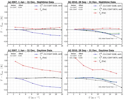
To examine the possibility of errors in Ts on the NWT
tower, we compareTsairto an aspirated temperature-humidity sensor (Tasp) as a function of wind speed (Fig. 8). It is
well-known thatTsaircan contain a significant bias relative to true T due to uncertainties in the sonic path length (Loescher et al., 2005; Mauder et al., 2007). Therefore, for presentation purposes, we adjustedTsair with an offset determined from the low wind speed value ofTsair−Tasp(the offsets used for
each CSAT are shown in Fig. 8). During both day and night and for ver3 and ver4 CSATs,Tsair−Taspshows a systematic
decrease on the order of 0.2 K as wind speed increases from around 8 to 15 m s−1(Fig. 8). This negativeTair
s error
corre-lated with increasingU explains the positiveHCSATerror in
0 2 4 6 8 10 12 14 16 18 −0.4
−0.2 0 0.2 0.4 0.6
0.8 Sensor OffsetCU CSAT 0.259
T
−
Ta
s
p
[
K
]
(a) 2007, 1 Jan − 31 Dec, Nighttime Data
T air
s , CU CSAT 0226, ver3 T
tc (Far)
0 2 4 6 8 10 12 14 16 18
−0.4 −0.2 0 0.2 0.4 0.6
0.8 Sensor OffsetCU CSAT −0.053
EOL CSAT −0.220
EOL Wind Tunnel Test −−−>
(b) 2010, 28 Sep − 31 Dec, Nighttime Data
T air
s , CU CSAT 0198, ver4
T air
s , EOL CSAT 0674, ver4 T
tc (Far)
0 2 4 6 8 10 12 14 16 18
−0.4 −0.2 0 0.2 0.4 0.6
0.8 Sensor Offset CU CSAT 0.303
T
−
Tas
p
[
K
]
U[m s−1]
(c) 2007, 1 Jan − 31 Dec, Daytime Data
T air
s , CU CSAT 0226, ver3 T
tc (Far)
0 2 4 6 8 10 12 14 16 18
−0.4 −0.2 0 0.2 0.4 0.6
0.8 Sensor Offset CU CSAT 0.180 EOL CSAT −0.005
EOL Wind Tunnel Test −−−>
U[m s−1]
(d) 2010, 28 Sep − 31 Dec, Daytime Data
T air
s , CU CSAT 0198, ver4
T air
s , EOL CSAT 0674, ver4 Ttc (Far)
Fig. 8. The (a, b) nighttime and (c, d) daytime mean temperature difference (T−Tasp) versus 21.5 m horizontal wind speedU.Taspis measured within a mechanically aspirated housing, andT is from either a humidity-corrected CSAT (Tsair) or a thermocouple (Ttc) as specified in the legend (also see Table 1). Only periods withU >1 m s−1are used.Tsairhas been adjusted toTaspusing an offset determined for 1< U <4 m s−1, which is shown in the upper left corner of each panel. The time period used is shown above each panel. The black lines are the ver3 (left panels) and ver4 (right panels) wind tunnel data shown in Fig. 7.
The nighttime thermocouple measurements can be used to check the quality of the aspirated temperature-humidity mea-surements. At night (Fig. 8a and b), theTtc−Taspdifference
is less than±0.1 K and independent of wind speed. How-ever, during the day (Fig. 8c and d), there is a well-known radiation effect onTtcthat causes it to be larger thanTaspby
about 0.6 K at low wind speeds but decreases to 0.2 K for high winds (e.g., Campbell, 1969; Burns and Sun, 2000; Fo-ken, 2008b). ThoughTtcis affected by radiation, we note that
the effect onw0T0
tcshould be small becausew0should not be
correlated with the radiation error.
3.4 Summary of Campbell Scientific, Inc. experiments
To further test the sonic temperature issues, independent ex-periments were performed at Campbell Scientific, Inc. (CSI), and we provide a brief summary of the results here. In the fu-ture, CSI will release information with additional details and recommendations for CSAT users.
The CSI experiments identified theTserrors to be caused
by a delayed detection of the sonic pulse which is blown off-axis by high winds normal to the sonic-path. Delayed de-tection of the pulse arrival time results in an overestimation of the transit time which leads to an underestimation of the speed of sound and thus also sonic temperature (e.g., Eq. 3). Although this error is qualitatively similar to the correction for the crosswind component, it is quantitatively different and directly related to the firmware estimation of the pulse arrival time.
The CSI experiments also confirmed that the magnitude of theTs errors differs for ver3 and ver4 of the firmware. The
0 2 4 6 8 10 12 14 16 18 −0.4
−0.2 0 0.2 0.4 0.6
0.8 Sensor OffsetCU CSAT −0.115
T
−
Ta
s
p
[
K
]
U[m s−1]
(a) 2009, 27 Sep − 31 Dec, Nighttime Data
T air
s , EOL CSAT 0674, ver3 Ttc (Far)
0 2 4 6 8 10 12 14 16 18
−0.4 −0.2 0 0.2 0.4 0.6
0.8 Sensor OffsetCU CSAT −0.089
U[m s−1]
(b) 2011, 22 Oct − 31 Dec, Nighttime Data
T air
s , EOL CSAT 0674, ver3 (OLD) Ttc (Far)
Fig. 9. As in Fig. 8, for the EOL CSAT 0674 ver3 using (a) newer and (b) older set of factory calibration coefficients. For details about the factory calibration dates, see Table 1. Daytime data are not shown.
occur. The best indicator of calibration drift causingTserrors
in ver3 is the “poor signal lock” flag in the CSAT diagnostic output (Campbell Scientific, Inc., 2010). Although larger, the ver4Tserrors are believed to be more stable with time than
ver3 errors.
To explore how the age of the calibration affects the NWT tower data, in October 2011, we changed the EOL CSAT (ver3) to an older set of ver3 calibration coefficients (Ta-ble 1). There is a slight improvement inTs−Tasp when the
newer calibration coefficients were used (Fig. 9). We can also observe a small improvement in theHCSAT−HTtcdifference
(e.g., compare Fig. 2a to f).
The sonic temperature is significantly more sensitive to transit time errors than wind speed, because the wind com-ponents are calculated from the difference between transit times in opposite directions along the path (Foken, 2008b). The wind speed error due to theTs error is estimated to be
on the order of 0.1 % at 20 m s−1and 0.3 % at 30 m s−1and result in a slight underestimation of true wind speed.
3.5 An empirical correction toHCSAT
A conceptual model of the CSAT heat flux error is that it de-pends on the covariance between vertical wind and erroneous fluctuations in the sonic temperature (Terr):
Herr
ρ cp
=w0T0 err =
∂w ∂uu
0 ∂Terr
∂u u
0
, (7)
where∂w/∂uis the slope of the relationship between vertical wind and the streamwise velocity component, and∂Terr/∂u
describes how the Ts error changes with respect to the
streamwise velocity. To determine∂w/∂u, we could perform a least-squares fit of instantaneous w andu measurements over a 30-min period. However, the optimal slope of∂w/∂u is also related tou0w0by
∂w ∂u =
u0w0
u0u0, (8)
where u0u0 is the variance of u. Because wind speed
in-creases with height,u0w0is negative. To determine∂T err/∂u,
we used a polynomial fit ofTsair−Tasp versus wind speed
(e.g., Figs. 7 and 8) which is also negative. The two nega-tive terms on the right side of Eq. (7) produce a posinega-tive heat flux error that is consistent with the NWT tower observations (i.e.,w0T0
s−w0Ttc0 >0). Substituting Eq. (8) into Eq. (7), the
empirical expression for theHCSATerror becomes
Herr
ρ cp
=
"
∂ A3u3+A2u2+A1u+A0
∂u
#
u0w0
=h3A3u2+2A2u+A1 i
u0w0, (9)
whereA3,A2,A1 andA0 are empirical coefficients
deter-mined by a 3rd-order polynomial fit betweenTsair−Taspand
wind speed. TheHCSATerror determined with Eq. (9) is
pos-itive as expected (Fig. 10a). Furthermore, HCSAT−Herr is
much closer toHTtcthanHCSAT(i.e., compare Fig. 10b with
Fig. 2d). This result shows how errors in the mean CSAT temperature are closely linked to the heat flux measurement errors. For some CSATs, a 2nd-order polynomial fit with Eq. (9) worked better than a 3rd-order fit (Fig. 10c). Other considerations when using Eq. (9) are the following: (1) the reference temperature sensor must not be significantly af-fected by changes in wind speed; (2) the coefficientsA3–A0
are determined over a specific time period and will only be valid if the CSAT calibration does not significantly change; (3) if∂Terr/∂uis stable with time, then an empirical
correc-tion can be used to correct historical fluxes measured by a particular CSAT; and (4) theHCSATerror will be unique for
each CSAT.
For the horizontal heat flux,u0w0in Eq. (9) gets replaced
byu0u0so the sign of the horizontal heat flux error is negative
(i.e.,u0T0 s−u0T
0
tc<0). Because u0w0< u0u0, the magnitude
0 2 4 6 8 10 12 14 16 18 20 −50
0 50 100 150 200 250 300 350
H err
[W m
−2
]
A
3 = −1.688e−05
A
2 = −6.255e−04
A
1 = 4.555e−03
A
0 = −5.050e−03 2150 cm CU CSAT 0198, ver4
(a) 2010, 30 Sep − 31 Dec
0 2 4 6 8 10 12 14 16 18 20
−150 −100 −50 0 50
−100 100
−50 150
0 50 100 150 200
(H
CSAT
−
H err
) −
H T
tc
[W m
−2
]
(H
CSAT
−
H err
) −
HT
tc
[W m
−2
]
=⇒ ⇐=
2150 cm CU CSAT 0198, ver4 2148 cm Ttc (Near)
(b) 2010, 30 Sep − 31 Dec
Day Night
0 2 4 6 8 10 12 14 16 18 20
−50 0 50 100 150 200 250 300 350
U[m s−1]
H err
[W m
−2
]
A
3 = 0
A
2 = −1.233e−04
A
1 = −1.073e−02
A
0 = 2.049e−02 2150 cm CU CSAT 0226, ver3
(c) 2007, 7 Sep − 31 Dec
0 2 4 6 8 10 12 14 16 18 20
−150 −100 −50 0 50
−100 100
−50 150
0 50 100 150 200
(H
CSAT
−
H err
) −
H T
tc
[W m
−2
]
(H
CSAT
−
H err
) −
HT
tc
[W m
−2
]
U[m s−1]
=⇒ ⇐=
2150 cm CU CSAT 0226, ver3 2198 cm Ttc (Far)
(d) 2007, 7 Sep − 31 Dec
Day Night
Fig. 10. The (a, c)HCSATsensible heat flux error (Herr) determined following Eq. (9) and (b, d) (HCSAT−Herr)−HTtc difference versus the 21.5 m horizontal wind speedUfor a ver4 (upper panels) and ver3 (lower panels) CSAT. In (a, c), the coefficientsA3–A0are determined from a fit ofTsair−Taspversus the wind speed. The difference shown in (b) and (d) can be compared toHCSAT−HTtc shown in Fig. 2d and e, respectively. See the Fig. 2 caption for other details.
3.6 Consideration of the surface energy balance
As mentioned in the introduction, Turnipseed et al. (2002) found that the nocturnal SEB closure fraction during high winds varied between 0.2 and 0.6. In Fig. 11, closure frac-tion (CF, see Sect. 2.3 for details) is calculated usingHCSAT
(CU 0226, ver3),HCSATempirically corrected withHerr(i.e.,
Eq. 9), andHTtc (Far). As one would expect, CF withHCSAT
closely matches the results of Turnipseed et al. (2002). At night (Fig. 11b), CF peaks at≈0.9 for moderate wind speed, and then becomes negative as wind speed increases (or as friction velocity increases as shown in Fig. 7 of Turnipseed et al., 2002). For low winds, drainage flows form at the NWT site (Yi et al., 2005; Burns et al., 2011) and result in near-zero nocturnal CF values due to decoupling, strong horizontal ad-vection of temperature, and practical difficulties with the flux calculation (e.g., Mahrt, 2010). These low-wind conditions require knowledge of horizontal advection for a more com-plete understanding (Sun et al., 2007; Yi et al., 2008).
During the day, closure fraction usingHTtc andHCSAT
di-verges atU≈6 m s−1(Fig. 11a). ForU >13 m s−1, CF with HCSATis close to 1. Knowing about theHCSATerror in high
winds (e.g., Fig. 3) suggests that the daytime CF approach-ing 1 is an artifact. In contrast, withHTtc, both the daytime
and nighttime CF values forU >6 m s−1are in reasonable agreement at CF≈0.65–0.75, and there is almost no depen-dence of CF on wind speed. Unless there is a physical rea-son for CF to change in higher wind speeds, usingHTtc
ap-pears more reasonable than HCSAT. With empirically
cor-rectedHCSAT, the day and night CF values in high winds
0 2 4 6 8 10 12 14 16 −0.4
−0.2 0 0.2 0.4 0.6 0.8
1 (a) Day
(
H
+
L
E
)
/
Ra
T
s, CU CSAT 0226, ver3 Ts, CU CSAT 0226, ver3 (+ H err )
T tc (Far)
0 2 4 6 8 10 12 14 16
−0.4 −0.2 0 0.2 0.4 0.6 0.8
1 (b) Night
U[m s−1]
(
H
+
L
E
)
/
Ra
Fig. 11. The surface energy balance closure fraction [CF = (H+ LE)/Ra] versus horizontal wind speed U for years 2006–2007 for (a) daytime and (b) nighttime conditions (Ra=Rnet−G is the available energy; see text for details). Rnet is measured with a REBS, model Q*7.1 radiometer. The temperature sensor used to calculateH is specified in the legend. The calculation ofHerrfor CSAT 0226 uses the coefficients shown in Fig. 10c. This figure is comparable to Fig. 7 in Turnipseed et al. (2002).
be taken into account (e.g., Leuning et al., 2012). Other fac-tors that might cause the lack of closure are discussed else-where (e.g., Turnipseed et al., 2002; Foken et al., 2011; Le-uning et al., 2012).
4 Conclusions
We compared sensible heat flux calculated using Campbell Scientific CSAT3 sonic anemometer temperature to heat flux calculated with a co-located thermocouple and found wind speed-dependent differences on the order of 250 W m−2 at high wind speeds (HCSAT> HTtc). These sensible heat flux
differences have been traced to errors in CSAT sonic temper-ature that occur in high winds. Independent tests at Campbell Scientific, Inc. determined that the sonic temperature errors are due to delayed detection of the sound pulse (which is blown off-axis by high winds normal to the transducer path) leading to an overestimation of the pulse transit time and an underestimation ofTs. Because the sound-pulse detection
de-pends on the firmware, the error is firmware-dependent. The error is significant for ver4 of the firmware and much smaller or negligible for ver3 of the firmware (as long as the ver3 CSAT factory calibration is accurate). Using a polynomial fit of theTs error as a function of wind speed, a conceptual
model was tested and found to correct most of theHCSAT
error. Also consistent with the conceptual model, the CSAT horizontal heat flux error is larger than the vertical heat flux error and with opposite sign. Campbell Scientific, Inc. is cur-rently working to better quantify the magnitude of the er-ror and will mitigate it with future hardware and/or software changes.
We also considered the impact of the CSAT heat flux er-ror on the closure fraction of the surface energy budget and found that using heat flux calculated with the thermocouple resulted in a more realistic closure fraction that was relatively insensitive to changes in wind speed. However, using spec-tral phase analysis, we observed that the time response of the thermocouple may lead to a slight underestimation ofH. In the future, a fast response, fine-wire temperature sensor could be deployed for an additional check of heat flux from the thermocouple.
Though our study examines one specific model of sonic anemometer, it is recommended that any sonic anemome-ter deployed in a location with strong winds includes a fast-response temperature sensor to ensure accurate sensible heat flux measurements. Furthermore, in a broader context, our temperature comparison shows the added value of
in-dependent, co-located, in-situ measurements in
environmen-tal research. Previous comparisons of sonic anemometers by Loescher et al. (2005) were very thorough, but performed the comparison up to a wind speed of≈6 m s−1, so any issues at higher wind speeds were undetected. This emphasizes an important advantage of long-term in-situ comparisons – they cover the range of the observation. In short, our study pro-vides a practical example of how valuable in-situ compar-isons can be in evaluating sensor performance.
Acknowledgements. We gratefully acknowledge assistance from
the scientists and staff at Campbell Scientific, Inc., especially Edward Swiatek for his support and interest. Don Lenschow, Gor-don Maclean, Steve Semmer, Jielun Sun and Steve Oncley provided useful discussions. We also thank Chris Golubieski (EOL CSAT and wind tunnel tests) and Jeff Beauregard (CU CSATs) for their assistance. Finally, we thank Erik Sahl´ee, Johannes Laubach, Thomas Foken, Heping Liu, Christof Ammann, and two anony-mous reviewers for comments that greatly improved the paper. The NWT tower has been supported by grants from the South Central Section of the National Institute for Global Environmental Change (NIGEC) through the US Department of Energy (BER Program, Cooperative Agreement No. DE-FC03-90ER61010) and from the National Science Foundation (NSF) Long-Term Research in Environmental Biology (LTREB). The National Center for Atmospheric Research (NCAR) is sponsored by NSF.
References
Aubinet, M., Grelle, A., Ibrom, A., Rannik, U., Moncrieff, J., Fo-ken, T., Kowalski, A. S., Martin, P. H., Berbigier, P., Bernhofer, C., Clement, R., Elbers, J., Granier, A., Grunwald, T., Morgen-stern, K., Pilegaard, K., Rebmann, C., Snijders, W., Valentini, R., and Vesala, T.: Estimates of the annual net carbon and water exchange of forests: The EUROFLUX methodology, Adv. Ecol. Res., 30, 113–175, 2000.
Barr, A. G., Morgenstern, K., Black, T. A., McCaughey, J. H., and Nesic, Z.: Surface energy balance closure by the eddy-covariance method above three boreal forest stands and implications for the measurement of the CO2flux, Agr. Forest Meteorol., 140, 322– 337, 2006.
Benedict, R.: Fundamentals of Temperature, Pressure, and Flow Measurements, Wiley-Interscience publication, 2nd Edn., Wiley, New York, 517 pp., 1977.
Berg, N. H.: Blowing snow at a Colorado alpine site: Measurements and implications, Arct. Alpine Res., 18, 147–161, 1986. Blanken, P. D., Black, T. A., Yang, P. C., Neumann, H. H., Nesic,
Z., Staebler, R., den Hartog, G., Novak, M. D., and Lee, X.: En-ergy balance and canopy conductance of a boreal aspen forest: Partitioning overstory and understory components, J. Geophys. Res., 102, 28915–28927, 1997.
Blanken, P. D., Black, T. A., Neumann, H. H., Den Hartog, G., Yang, P. C., Nesic, Z., Staebler, R., Chen, W., and Novak, M. D.: Turbulent flux measurements above and below the overstory of a boreal aspen forest, Bound.-Lay. Meteorol., 89, 109–140, 1998. Burns, S. P. and Sun, J.: Thermocouple temperature measurements
from the CASES-99 main tower, in: Proceedings of the 14th Symposium on Boundary Layer and Turbulence, Amer. Meteor. Soc., Snowmass, Colorado, 7–11 August 2000, 358–361, 2000. Burns, S. P., Sun, J., Lenschow, D. H., Oncley, S. P., Stephens, B. B.,
Yi, C., Anderson, D. E., Hu, J., and Monson, R. K.: Atmospheric stability effects on wind fields and scalar mixing within and just above a subalpine forest in sloping terrain, Bound.-Lay. Meteo-rol., 138, 231–262, doi:10.1007/s10546-010-9560-6, 2011. Burns, S. P., Horst, T. W., Blanken, P. D., and Monson, R. K.:
Using sonic anemometer temperature to measure sensible heat flux in strong winds, Atmos. Meas. Tech. Discuss., 5, 447–469, doi:10.5194/amtd-5-447-2012, 2012.
Campbell, G. S.: Measurement of air temperature fluctuations with thermocouples, Tech. Rep. ECOM-5273, Atmospheric Sciences Laboratory, White Sands Missile Range, 10 pp., 1969.
Campbell Scientific, Inc.: CSAT3 Three Dimensional Sonic Anemometer Manual (Revision 6/10), Campbell Scientific, Inc., Logan, Utah, 70 pp., 2010.
Farahmand, K. and Kaufman, J. W.: Experimental measurement of fine thermocouple response time in air, Exp. Heat Transfer, 14, 107–118, doi:10.1080/08916150120876, 2001.
Foken, T.: Bestimmung der Schneedrift mittels Ultraschal-lanemometern (Detection of snow drift with sonic anemometers), Ann. Meteorol., 37, 451–452, 1998.
Foken, T.: The energy balance closure problem: An overview, Ecol. Appl., 18, 1351–1367, 2008a.
Foken, T.: Micrometeorology, Springer, Heidelberg, 308 pp., 2008b. Foken, T., Aubinet, M., Finnigan, J. J., Leclerc, M. Y., Mauder, M., and Paw U, K. T.: Results of a panel discussion about the en-ergy balance closure correction for trace gases, B. Am. Meteorol. Soc., 92, ES13–ES18, 2011.
Franssen, H. J. H., St¨ockli, R., Lehner, I., Rotenberg, E., and Seneviratne, S. I.: Energy balance closure of eddy-covariance data: A multisite analysis for European FLUXNET stations, Agr. Forest Meteorol., 150, 1553–1567, doi:10.1016/j.agrformet.2010.08.005, 2010.
Friebel, H. C., Herrington, T. O., and Benilov, A. Y.: Evaluation of the flow distortion around the Campbell Scientific CSAT3 sonic anemometer relative to incident wind direction, J. Atmos. Ocean. Tech., 26, 582–592, doi:10.1175/2008JTECHO550.1, 2009. Friehe, C. A. and Khelif, D.: Fast-response aircraft temperature
sen-sors, J. Atmos. Ocean. Tech., 9, 784–795, 1992.
Friehe, C. A., Shaw, W. J., Rogers, D. P., Davidson, K. L., Large, W. G., Stage, S. A., Crescenti, G. H., Khalsa, S. J. S., Green-hut, G. K., and Li, F.: Air-sea fluxes and surface-layer turbu-lence around a sea-surface temperature front, J. Geophys. Res., 96, 8593–8609, 1991.
Fuehrer, P. L. and Friehe, C. A.: Flux corrections revisited, Bound.-Lay. Meteorol., 102, 415–457, 2002.
Fuehrer, P. L., Friehe, C. A., and Edwards, D. K.: Frequency-response of a thermistor temperature probe in air, J. Atmos. Ocean. Tech., 11, 476–488, 1994.
Garratt, J. R.: The Atmospheric Boundary Layer, Cambridge Uni-versity Press, Cambridge, 316 pp., 1992.
Grelle, A. and Burba, G.: Fine-wire thermometer to correct CO2 fluxes by open-path analyzers for artificial density fluctuations, Agr. Forest Meteorol., 147, 48–57, 2007.
Grelle, A. and Lindroth, A.: Eddy-correlation system for long-term monitoring of fluxes of heat, water vapour and CO2, Global Change Biol., 2, 297–307, 1996.
Hignett, P.: Corrections to temperature-measurements with a sonic anemometer, Bound.-Lay. Meteorol., 61, 175–187, 1992. Horst, T. W. and Lenschow, D. H.: Attenuation of scalar fluxes
mea-sured with spatially-displaced sensors, Bound.-Lay. Meteorol., 130, 275–300, 2009.
Kaimal, J. C. and Businger, J. A.: A continuous wave sonic anemometer-thermometer, J. Appl. Meteorol., 2, 156–164, 1963. Kaimal, J. C. and Finnigan, J. J.: Atmospheric Boundary Layer Flows: Their Structure and Measurement, Oxford University Press, New York, 289 pp., 1994.
Kaimal, J. C. and Gaynor, J. E.: Another look at sonic thermometry, Bound.-Lay. Meteorol., 56, 401–410, 1991.
Lanzinger, E. and Langmack, H.: Measuring Air Temperature by using an Ultrasonic Anemometer, in: Technical Conference on Meteorological and Environmental Instruments and Methods of Observation (TECO-2005), WMO Tech. Doc. No. 1265; IOM Report No. 82, World Meteorological Organization, Geneva, Switzerland, p. P3(9), 2005.
Laubach, J.: Charakterisierung des turbulenten Austauschs von W¨arme, Wasserdampf und Kohlendioxid ¨uber niedriger Vege-tation anhand von Eddy-Korrelations-Messungen (Characteriza-tion of the turbulent exchange of heat, water vapor, and carbon dioxide over low vegetation by means of eddy correlation mea-surements), Ph.D. thesis, University of Leipzig, Leipzig, Ger-many, 1995.