Multiple-Instabilities in Magnetized Plasmas with Density
Gradient and Velocity Shears
Makoto SASAKI
1,2), Naohiro KASUYA
1,2), Shinichiro TODA
3), Takuma YAMADA
2,4),
Yusuke KOSUGA
1,2), Hiroyuki ARAKAWA
5), Tatsuya KOBAYASHI
3), Shigeru INAGAKI
1,2),
Akihide FUJISAWA
1,2), Yoshihiko NAGASHIMA
1,2), Kimitaka ITOH
2,3,6)and Sanae-I ITOH
1,2)1)Research Institute for Applied Mechanics, Kyushu University, Kasuga 816-8580, Japan 2)Research Center for Plasma Turbulence, Kyushu University, Kasuga 816-8580, Japan
3)National Institute for Fusion Science, Toki 509-5292, Japan 4)Faculty of Arts and Science, Kyushu University, Fukuoka 819-0395, Japan
5)Teikyo University, Fukuoka 836-8505, Japan
6)Institute of Science and Technology Research, Chubu University, Kasugai 487-8501, Japan (Received 24 May 2017/Accepted 28 August 2017)
Multiple free energy sources for instabilities coexist in magnetized plasmas with density gradient and veloc-ity shear. Linear stabilities are investigated, and the mutual relation between resistive drift wave, D’Angelo mode and flute mode is systematically clarified. By evaluating the linear growth rates, dominant instability is catego-rized in a parameter space. The parallel wavenumber spectrum could be used as a guideline for the identification of the instabilities.
c
2017 The Japan Society of Plasma Science and Nuclear Fusion Research
Keywords: stability, flow shear, turbulence, transport, drift wave, D’Angelo mode, flute mode DOI: 10.1585/pfr.12.1401042
1. Introduction
Multiple free energy sources for instabilities coexist in magnetized plasmas with density gradient and velocity shear. Density and temperature gradients destabilize drift wave type instabilities such as resistive drift wave, and ion temperature gradient mode [1]. Inhomogeneous flows such as poloidal mean sheared flow, zonal flow and toroidal rotations are driven intrinsically [2–5] and/or externally [6–8]. Strong inhomogeneity of the perpendicular flow can be a free energy source of the KelvHelmholtz (KH) in-stability [9–12] and interchange mode [13, 14]. When the parallel flow shear becomes strong, the parallel compres-sion for ion acoustic waves can become negative to drive KH-type instability. This instability is called the D’Angelo mode [15, 16], which has been observed in basic plasma experiments [17]. Turbulence simulation and theory sug-gest the importance of the D’Angelo mode at scrape off layers and spherical tokamaks [18, 19]. The coexistence of the D’Angelo mode and drift wave has been observed [17]. On one hand, the drift wave induces the particle transport that reduces the density gradient, and simultaneously drive the momentum transport to form the parallel flow [20]. On the other hand, the D’Angelo mode relaxes the parallel flow gradient by momentum transport, and steepens the density gradient via the particle pinch effect [16]. Thus, a direct cross-interference between the particle and momen-tum transport occurs in a system where instabilities due to
author’s e-mail: [email protected]
the density gradient and the flow inhomogeneities coex-ist. Therefore, the experimental identification of the insta-bilities among such modes is becoming increasingly im-portant. Although the characteristics of these instabilities have been thoroughly investigated individually, the mutual relations between such instabilities need to be clarified in a systematic study.
Hence, in this study, we investigate the linear sta-bility of magnetized plasmas in the presence of a den-sity gradient, perpendicular flow curvature and parallel flow shear. The relationships between the resistive drift waves, D’Angelo and flute modes are clarified. In addition, a guideline for identifying such instabilities is presented here. The following parts of the paper are organized as follows. The basic model is described in Sec. 2, and ana-lytical formulas for each instability are presented in Sec. 3. In Sec. 4, the mutual relations between the instabilities are described, and a summary is presented in Sec. 5.
2. Model
We consider slab plasmas with a density gradient, per-pendicular flow curvature and parallel flow shear in a sim-ple geometry where the magnetic field is homogeneous. This situation corresponds to those of the basic plasma ex-periments [6, 7, 17]. The direction of the magnetic field is chosen to bez-direction, and the direction of the gradient of the density is set to bex-direction. A three-field reduced fluid model is used, which is based on the
Hasegawa-c
Wakatani model with coupling of the ion parallel flow [16], where the field f =(N, φ,V)T
is calculated. Here, the den-sityN, electrostatic potentialφ, and the ion parallel veloc-ityVare normalized by mean density, electron temperature and sound speed, respectively. We divide f into its mean and fluctuating components as f =f+˜f. We keep the terms due to spatial inhomogeneities off(which causes the instabilities). In this study, we focus on the linear prop-erties of the instabilities with multiple free energy sources; hence, we investigate the linearized equation. The basic model equation, and the derivation of the linearized equa-tion are given in Appendix.A. The linearized equaequa-tion is as follows,
∂t˜f+L˜f =0. (1)
The linear operatorLis given as
L=L1+L2, (2)
L1=
⎛ ⎜⎜⎜⎜⎜ ⎜⎜⎜⎜⎝−D∇
2
−μN∇2⊥ D∇2 ∇
−D∇−2
⊥ ∇2 D∇−⊥2∇2+ν−μφ∇2⊥ 0 ∇ 0 ν−μV∇2⊥
⎞ ⎟⎟⎟⎟⎟ ⎟⎟⎟⎟⎠,
(3)
L2=
⎛ ⎜⎜⎜⎜⎜ ⎜⎜⎜⎜⎝
V∇+∂xφ∂y −∂xN∂y 0 0 −∂xφ∂y+I 0 0 −∂xV∂y V∇+∂xφ∂y
⎞ ⎟⎟⎟⎟⎟ ⎟⎟⎟⎟⎠,
(4) whereL1 is the operator that describes the geometry and physical properties of the plasma, and L2 is related to the spatial inhomogeneity of the density, the electrostatic potential, and the ion parallel flow. The density gradi-ent, ∂x
N, the parallel flow shear, ∂x
V, and the cur-vature of the azimuthal flow,∂3
x
φ, drive the drift wave, the D’Angelo mode and the KH instability, respectively. The ion-neutral collision frequency is denoted byν, D = A/(νei +νen) is the parallel diffusivity of electrons, A is the ion-electron mass ratio,νeiis the electron-ion collision frequency, νen is the electron-neutral collision frequency, andμN, μφ, μV are the viscosities. Here, the time and space are normalized by the ion cyclotron frequency and the ion sound Larmor radius, respectively. The operatorI, which is important for driving the flute mode, is given as
I=∂3x
φ∇−2
⊥∂y+∂xN∇−⊥2∂x∂t
+∂xN∂xφ∇⊥−2∂x∂y−∂xN∂2x
φ∇−2
⊥ ∂y. (5) Assuming the function form of the fluctuations as ˜f =
kfkexp(−iωt+ik·x)+c.c, we obtain the eigen equation as
j
Δi jfk,j=0, (6)
Δ =−iωI+Lk. (7)
Here,Lk is calculated fromL, where the derivatives, ∂t and∇are replaced by−iωandik. The dispersion relation is obtained as
detΔ =0. (8)
From the eigen equation, the eigenfunctions of the density and the parallel flow fluctuations are formally written as
˜
Nk= Δ32Δ13−Δ33Δ12
Δ11Δ33−Δ13Δ31 ˜
φk, (9)
˜
Vk= Δ31Δ12−Δ11Δ32
Δ11Δ33−Δ13Δ31 ˜
φk. (10)
The dispersion relation shown in Eq. (8) includes the free energy sources for the instabilities due to∂x
N,∂x
Vand
∂3 x
φ
.
3. Analytical Formulas for
Instabili-ties
Based on the linear dispersion relation (8), we investi-gate the relationships between the multiple instabilities. In order to obtain analytical insights, we derive expressions for the eigenfrequencies of each instability in a limit of
ν, μN, μφ, μV → 0, keeping the effects of the flow and the density gradient.
Equation (8) can be expressed in a limit of
ν, μN, μφ, μV →0.
Dk2 Ω 1+k−⊥2Ω +kV−k⊥−2ω∗−iI
+kkyk⊥−2∂xV−k2k−⊥2
+ik2−Ω2 Ω +kV−iI=0, (11) whereΩ =ω−ky∂xφ−kVis the eigenfrequency with the Doppler shift by the perpendicular and parallel flows, andω∗=−ky∂xNis the electron drift frequency. Cases ofk0
Equation (11) can be rewritten as
Ω2−αΩ−β−i(Ω)=0, (12)
α=ω∗−k2⊥k+ik2⊥I
1+k2
⊥ ,
(13)
β=−kky∂x
V+k2
1+k2
⊥ ,
(14)
(Ω)= k 2
⊥
Dk2
1+k2
⊥
Ω2−k2
Ω+kV−iI. (15)
AssumingDk2 ω and neglecting the term I, we treat
(Ω) perturbatively. We expand the solution asΩ = Ω(0)+
Ω(1)+. . .with the ordering ofO(Ω/Dk2
). The lowest and
first order solutions are obtained as
Ω(0)= 1 2
α±α2+4β
, (16)
Ω(1)=i (Ω(0))
2Ω(0)−α. (17)
i)β→0
solution can be expressed as
ω≈ ω∗
1+k2
⊥ −k2⊥k
V
1+k2
⊥
+ky∂xφ+kV
+ik
2
⊥ω∗ω∗+kV Dk2
1+k2
⊥
2 , (18)
which corresponds to the resistive drift wave (including the effects of the parallel and perpendicular flows). The real frequency is Doppler shifted by the velocity field as seen in the third and fourth terms of the right hand side of Eq. (18). The parallel mean flow induces an asymmetry in the growth rate with respect to the sign ofk. The growth rate of the mode satisfyingkV>0 becomes large, and that of the mode withkV<0 becomes small.
ii)|β|> α/4, β <0
The D’Angelo mode becomes unstable when the parallel flow shear satisfiesα2+4β <0, which can be expressed in terms of the parallel velocity shear as
kky∂x
V>k2+
ω∗−k2⊥kV2
41+k2
⊥
. (19)
This condition corresponds toα2+4β < 0, where the un-stable branch is obtained fromΩ(0). The eigenfrequency of the unstable branch is derived as
ω≈ ω∗
21+k2
⊥
− k2⊥kV
21+k2
⊥
+ky∂x
φ+
kV
+ 2(Ω(0))
|α2+4β| +i 1 2
|α2+4β|. (20)
The effect of(Ω(0)) contributes to the real frequency un-like the drift wave case. The necessary condition for the D’Angelo mode to become unstable is Eq. (19), where the
k-spectrum of the D’Angelo mode is completely asymme-try with respect to the sign ofk.
Case ofk=0
The dispersion relation of the mode withk=0 is obtained as
Ω =iI. (21)
The eigenfrequency can be expressed as
ω≈ky
∂xφ+k⊥−2
∂3 x
φ−∂
xN∂2x
φ
+i−kxkyk⊥−4∂xN∂3x
φ,
(22) where k−2
⊥ kx∂x
N 1 is assumed. When
kxky∂x
N∂3 x
φ <
0 is satisfied, the mode withk = 0 becomes linearly unstable due to the coupling of∂x
N
and ∂3 x
φ. Note that this instability is different from the KH instability and the rotation driven interchange mode (RDI) [13]. In order to explain the relation of the
instability obtained here with the conventional KH and RDI modes, the eigenequation Eq. (6) is rewitten as
k2⊥φ˜k+∂x
Nikxφ˜k
− ky ω−ky∂xφ
∂3 x
φ+∂
xN∂2x
φφ˜
k=0. (23) Here, the KH and RDI modes are destabilized by the third and fourth terms, respectively. Note that the KH and RDI modes are stable when the radial eigenfunction is a plane wave, eikxx. Radial eigenmode analysis is necessary to in-clude these instabilities. In this study, we assume the the function form as eikxx, and remove the KH and RDI. As seen from the dispersion relation Eq. (22), the instability we are considering is driven by the coupling between the density and vorticity gradients.
The eigenfunctions of the density and parallel veloc-ity fluctuations are explained in Appendix. B; these are important for the experimental identification of the insta-bilities. The characteristics of the quasi-linear fluxes of the particle and parallel momentum are also discussed in this appendix.
4. Mutual Relations between the
In-stabilities in Parameter Space
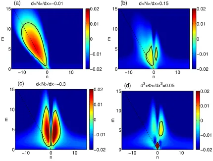
We consider situations where several free energy sources for the instabilities coexist. The dispersion relation in Eq. (8) is a cubic equation, implying that it has three so-lutions. In order to understand the relationships between the drift wave, D’Angelo and flute modes, the dispersion relation is calculated as shown in Fig. 1. In the case of the pure drift wave, Fig. 1 (a), (c), which corresponds to the condition that the parallel flow shear and the gradient of the vorticity are not present, the purely symmetric solu-tion inkis obtained. When the parallel flow shear exists, the symmetry inkis violated, and the unstable D’Angelo mode appears where the real frequency of the drift wave and the ion sound wave degenerate. The linearly unstable flute modek =0 appears and the D’Angelo mode disap-pears when the vorticity gradient∂3x
φ
is present as shown in Fig. 1 (e), (f).
In order to obtain a guideline for identifying the in-stability, we present the characteristics of the mode spec-tra based on the linear growth rate. The parameters here are chosen to be similar to those of a basic plasma exper-iment on PANTA [17]. The plasma radius isa =10 [cm], the device length inz-direction is λ = 4 [m], and V =
0.7,kx=1/a, μN =μV =10−2, μφ=10−4, νei=500, νen= 10, ν = 3.5 ×10⁻². Treating ∂
xN, ∂xV and ∂3x
φ
as parameters, the linear growth rate in the mode number space is shown in Fig. 2, which is expected to correspond to the mode spectra. We use the relation, ky = m/a/2 and k = 2πn/λ, where m and n are the perpendicular and parallel mode numbers, respectively. Figures 2 (a)-(c) are obtained by changing the density gradient with
∂x
V = −0.15, and∂3 x
Fig. 1 Dispersion relations; (a), (b) pure drift wave, (c), (d) D’Angelo mode and drift wave, (e), (f) Flute and drift wave. Each case is
calculated with (∂x
N, ∂3
x
φ)=(0,0) for (a), (b), (−0.2,0) for (c), (d), and (−0.2,0.02) for (e), (f).
Fig. 2 Growth rateγin (m,n)-space: (a) D’Angelo mode case, (b) intermediate mode of D’Angelo mode and drift wave, and (c) drift
wave dominant case, and (d) flute mode dominant case.
characteristic spectrum of the D’Angelo mode, where the modes withkky∂x
V > 0 are excited. This spectrum is asymmetry inn-space, where then-spectrum width is wide (Δn ∼10). Here, the regions where the linear growth rate is positive are indicated by the closed black lines. Note that the other area is filled with damped waves. The black broken line corresponds to the condition for the most un-stable modes, k = ky∂xV/2 [16]. When the density
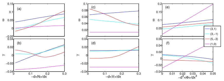
Fig. 3 Change of eigenfrequency and growth rate with the change of (a) (b) density gradient, (c) (d) parallel flow shear, and (e) (f) gradient of electrostatic potential curvature.
mode and the drift wave corresponds to Fig. 2 (b). The drift wave is observed atn>0, and the intermediate mode ap-pears atn<0. Figure 2 (d) corresponds to the flute mode, which is obtained with∂3x
φ=
0.05, ∂xV=0. The flute mode withn =0 coexists with the drift wave withn >0. In this case, the interference between the flute mode and the drift wave is expected.
Figure 3 illustrates the dependence of the real fre-quency and the growth rate of the instabilities on spatial inhomogeneities. The representative modes are selected as (m,n)=(3,±1),(5,−3),(1,0) for the drift wave, D’Angelo and flute modes, respectively. The dependence on the den-sity gradient is shown in Fig. 3 (a) and (b), which is cal-culated by using∂xV = −0.2, ∂3x
φ =
0.05. The fre-quency of the modes other than the flute mode increases with the density gradient. The growth rate of the drift wave constantly increases with−∂x
N. The growth rate of the D’Angelo mode decreases in the small density gra-dient cases, and increases to be drift wave-like mode in the high density gradient cases. Since the drift wave with the negativensatisfies the conditionkyk∂x
V>0, this mode is weakly driven by the parallel flow shear in addition to the density gradient. Thus, the mode withn=−1 becomes most unstable at the intermediate region of the D’Angelo mode dominant state and the drift wave dominant state. Figures 3 (c) and (d) show the dependence on the parallel flow shear. The real frequencies of the D’Angelo mode and the drift wave with the negativenbecome small with the parallel flow shear, and that of the drift wave with the posi-tivenincreases. The growth rates of the drift waves are not sensitive to the parallel flow shear. The dependence on the gradient of the potential curvature is shown in Figs. 3 (e) and (f). The frequency of the every instability increases with∂3
x
φ
. The growth rate of the drift waves becomes small with∂3
x
φ
, while that of the D’Angelo mode is not sensitive.
We focus on the behavior of the most unstable mode in the parameter space of∂x
N, ∂x
V, and∂3 x
φ
. Figure 4 illustrates the parallel mode number of the most unstable
Fig. 4 Parallel mode number of the most unstable mode in pa-rameter space. The drift wave and the D’Angelo mode are denoted by ’DW’ and ’DA’, respectively.
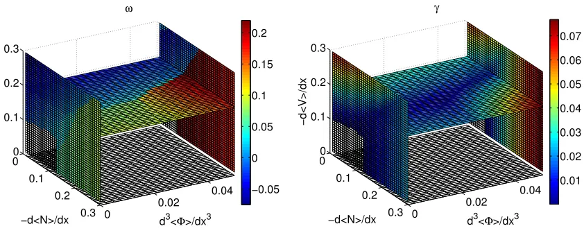
mode. In the region where the D’Angelo mode is domi-nant, the parallel mode number isn <−2, and isn =1 in the drift wave dominant region. In its intermediate region, the drift wave withn =−1 can be most unstable. When the gradient of the potential curvature becomes large, the dominant mode changes fromn =1 ton =0. The effect of the perpendicular flow on the D’Angelo mode is not so sensitive that the transition to the flute mode is not obtained in the weak density gradient cases. The real frequency and the growth rate of the most unstable mode are shown in Fig. 5. Although the boundary of the each dominant insta-bility is not clear for the real frequency and growth rate as shown in Fig. 5, the boundary for the parallel mode num-ber is clear. Thus, the parallel mode numnum-ber is the key parameter for determining the type of the instability.
Fig. 5 (a) Real frequency and (b) growth rate of the most unstable mode in parameter space.
Table 1 Characteristics of each instability, wheremandnare the azimuthal and axial mode numbers.
necessary condition n Δn: spectrum width
drift wave nV>0 n=1 or−1 small
D’Angelo mode nmV>0 |n|: large large
Flute mode ∂3
x
φ
: large n=0 small
for identifying the instabilities. Note that, in addition to the modes shown in the table, there is the intermediate mode in the region where the growth rates of the D’Angelo mode and the drift wave are similar. The sign of the par-allel mode number of the intermediate mode is same as the D’Angelo mode, while the absolute mode number is
|n|=1, similar to the drift wave.
5. Summary
We systematically investigate the linear analyses of in-stabilities in the inhomogeneous magnetized plasmas with a density gradient, and parallel and perpendicular mean flows. The dispersion relation, which includes the multi-ple instabilities, is derived. The relationships between the resistive drift wave, D’Angelo and flute modes are clari-fied. Characteristics of the expected fluctuation spectra are discussed based on the linear growth rates. The dominant instability is categorized in a parameter space. The paral-lel mode number is the important parameter for identifying such instabilities.
Acknowledgments
This work was partly supported by a grant-in-aid for scientific research of JSPS, Japan (16K18335, 16H02442, 15H02155, 17H06089, 17K06994) and by the collaboration programs of NIFS (NIFS15KNST089, NIFS17KNST122) and of the RIAM of Kyushu Univer-sity.
Appendix A. Derivation of Linear
Dispersion Relation
The Hasegawa-Wakatani model with coupling of the ion parallel flow is considered. The basic model equation is given by
∂tf+L1f =N(f,f), (A.1) where the linear operatorL1, and the nonlinear termNare given as
L1=
⎛ ⎜⎜⎜⎜⎜ ⎜⎜⎜⎜⎝−D∇
2
−μN∇2⊥ D∇2 ∇
−D∇−⊥2∇2 D∇⊥−2∇2+ν−μφ∇2⊥ 0 ∇ 0 ν−μV∇2⊥
⎞ ⎟⎟⎟⎟⎟ ⎟⎟⎟⎟⎠,
(A.2)
N(f,f)=
⎛ ⎜⎜⎜⎜⎜ ⎜⎜⎜⎜⎝
N, φ−V∇N
∇−2
⊥ ∇2⊥φ, φ − ∇−⊥2∇N·dt∇⊥φ
V, φ−V∇V
⎞ ⎟⎟⎟⎟⎟
⎟⎟⎟⎟⎠, (A.3)
where [φ, . . .] = ∂xφ∂y−∂yφ∂x is the convective deriva-tive. We divide f into the mean and fluctuating compo-nents as f =f+˜f. Spatial inhomogeneity of f causes the instabilities; the density gradient, perpendicular flow curvature and the parallel flow shear destabilize the resis-tive drift waves, the flute modes and the D’Angelo modes, respectively. The nonlinear term is linearized as
N(f,f)≈ −L2(
f) ˜f. (A.4)
Appendix B. Eigenfunctions and
Quasi-Linear Fluxes of Particles
and Momentum
The quasi-linear fluxes of the particle and parallel mo-mentum are evaluated by using the linear eigenfunction, Eqs. (9) and (10).
Case ofk0
Neglecting the viscositiesμN = μφ = μV = 0, we derive the analytical expressions of the eigenfunctions with the assumptionDk2
ωas
˜
Nk≈
1+ i
Dk2
Ω
Ω(Ω−ω∗)+kky∂x
V−k2 φ˜k, (B.1) ˜
Vk≈
k−ky∂xV
Ω +i k
Dk2
Ω2
Ω(Ω−ω∗)−k2 +kky∂xVφ˜k. (B.2) The phase differences of the density and parallel flow fluc-tuations with the electrostatic potential are governed by Eqs. (B.1) and (B.2). The perpendicular flow affects the phase differences of the density and parallel flow through the Doppler shift. The parallel mean flow speed affects the phase relation through the Doppler shift, while the parallel flow shear directly affects the phase relations. The paral-lel flow fluctuation becomes large with the increase of the parallel flow shear as was observed in [21]. By using the above expressions, the quasi-linear fluxes are obtained as
Γx=
˜
Nv˜x
, ≈
k
ky Dk2
Ω
Ω(ω∗−Ω)−kky∂x
V+k2|φ˜k|2, (B.3)
Πxz=˜vxV˜,
≈
k
kky Dk2
Ω2
Ω(ω∗−Ω)−kky∂xV+k2
|φ˜k|2, (B.4) where the radial velocity fluctuation is evaluated from the
E×Bdrift as ˜vx=−ikyφ˜. The first term of the particle flux in Eq. (B.3) becomes positive when the drift wave is im-portant, which leads to the outward particle flux. The sec-ond term contributes to the inward flux when the D’Angelo mode is important,kky∂xV>0. The sign of the net par-ticle flux is determined by the competition of these effects. Concerning to the parallel momentum flux, the first term, which is important for the drift wave case, can be positive and negative depending on the breaking of the symmetry in the sign ofkky. The second term, which is important for the D’Angelo mode case, is always negative, so that this term works as the relaxation of the flow profile. The detailed formulation of the net momentum flux is reported in [22].
Case ofk=0
Similarly, the eigenfunction of the flute mode is obtained as
˜
Nk≈ ω∗
Ωφ˜k, (B.5)
˜
Vk≈ −
ky∂x
V
Ω φ˜k. (B.6)
Then the fluctuation driven fluxes are derived as
Γx≈ −
k
k2 yγ
|Ω|2|φ˜k| 2∂
xN, (B.7)
Πxz≈ −
k
k2 yγ
|Ω|2|φ˜k| 2∂
xV, (B.8)
whereγ=ImΩ. Thus, in the case of the linearly unstable flute mode, the direction of the particle and parallel mo-mentum fluxes are outward, and the density profile flattens. The transport coefficients of the particle and momentum fluxes take the same value in this case.
Depending on the type of instability, the effects of the fluctuation driven fluxes of the particles and momen-tum differ, and the properties of the background density and velocity field are sensitively affected. Since the fluc-tuation driven fluxes are determined from the summation of all excited modes, the competition and coexistence of the multiple instability become important to determine the background profiles. Nonlinear simulations are necessary for the study on the interaction between multiple instabili-ties [23].
[1] W. Horton, Rev. Mod. Phys.71, 735 (1999).
[2] P.H. Diamondet al., Plasma Phys. Control. Fusion47, R35
(2005).
[3] A. Fujisawaet al., Nucl. Fusion49, 013001 (2009).
[4] J.E. Riceet al., Nucl. Fusion47, 1618 (2007).
[5] O.D. Gurcanet al., Phys. Plasmas14, 042306 (2007).
[6] T. Yamadaet al., Nucl. Fusion54, 114010 (2014).
[7] T.A. Carteret al., Phys. Plasmas16, 012304 (2009).
[8] D.M. Fisheret al., Phys. Plasmas24, 022303 (2017).
[9] W. Hortonet al., Phys. Fluids30, 3485 (1987).
[10] W. Hortonet al., Phys. Plasmas12, 022303 (2005).
[11] H. Hasegawaet al., Nature430, 755 (2004).
[12] E.J. Kimet al., Phys. Plasmas9, 4530 (2002).
[13] P. Popovichet al., Phys. Plasmas17, 102107 (2010).
[14] B.N. Rogerset al., Phys. Rev. Lett.104, 225002 (2010).
[15] N. D’Angelo, Phys. Fluids8, 1748 (1965).
[16] Y. Kosugaet al., Plasma Fusion Res.10, 3401024 (2015).
[17] S. Inagakiet al., Sci. Rep.6, 22189 (2016).
[18] X. Garbetet al., Phys. Plasmas6, 3955 (1999).
[19] W.X. Wanget al., Nucl. Fusion55, 122001 (2015).
[20] P.H. Diamond, Nucl. Fusion53, 104019 (2013).
[21] N. Dupertuis et al., Plasma Fusion Res. 12, 1201008
(2017).
[22] Y. Kosuga, S.-I. Itoh and K. Itoh, Plasma Fusion Res.11,
1203018 (2016).