©2014 JNAS Journal-2014-3-3/260-267 ISSN 2322-5149 ©2014 JNAS
Analysis of rectangular thin plates by using finite
difference method
Ali Ghods
*and Mahyar Mir
Department of civil , Zahedan Branch, Islamic Azad University, Zahedan, Iran
Corresponding author:Ali Ghods
ABSTRACT: This paper presents an investigation into the performance evaluation of Finite Difference (FD) method in modeling a rectangular thin plate structure. In case of complex and big construction systems subjected to the arbitrary loads, including a complex boundary conditions, solving of differential equations by analytical methods is almost impossible. Then the solution is application of numerical methods. The differential equations are discretized by means of the finite difference method which are used to determine the in-plane stress functions of plates and reduced to several sets of linear algebraic simultaneous equations. In the end, A problems is solved which illustrate the potential of the method for predicting the finite stress, deflection and farther directions of investigations are given. Finally, it was found that the finite difference method selection is desired to model thin plates structure.
Keywords: Finite Difference Method, Failure Thoeries, Thin Plate, Distortion Energy Theory, Strain.
INTRODUCTION
Thin plates are structural elements that their thickness is smaller than its two dimensions. Among practical examples to describe the dimensions of these plates are roof, building windows, flat part of a table, manhole thin covering and panels. plates are divided into two categories: thin plates with large deflections and thick plates (Boot, 1988 and Krysko, 2011). In thin plates, deflections and deformation of structural elements are usually considered and for ease of work, in structural plates, their deflections are studied under loading conditions.
Linear theory is used in describing the lateral displacements or small deformation under loading and this method is used in the analysis of thin plates under lateral loads. If plates’ deflections are large, this method cannot be used (Kaiser, 1936).
If plates’ deflections are large, deflection of middle of the plate is increased then, the linear method cannot be applied for determining the deflection of these plates. These errors are large and obtained linear solutions including displacement and stress are contrary to experimental observations.
Thus the non-linear theory for plates is developed by Von Karman and was used in the analysis of thin plates. Linear difference equations in plates were presented for the first time in 1910 by Von Karman then Kirchhoff used these equations for large deformations.
He also studied plates’ internal forces with external deformations and stated simultaneously their relationship with each other. The simplest application of this method is in thin rectangular plates. Then In 1936, Kaser solved a uniformly laterally loaded, simply supported, square plate problem (Kan, 1967 and Kim, 2002).
He used finite difference method and supported solutions to solve this problem and analyzing experimental results in analyzing this plate. In recent years, studies were done in connection with finite element of flexure problems such as analysis of large displacements, plate vibration, problems related to stress, etc (Wang and Wu , 2011; Zhang, 2010).
An approximate method for the analysis of plates using the finite difference method were presented by Bhaumik and Hanley for uniformly loaded rectangular plate. However, in this study they assumed that the behavior of each point of the mesh in the thickness is fully elastic or fully plastic.
261 mentioned, enough studies have not been done in examining the application of finite difference method in modeling and simulating thin plates, Therefore, in this study, the finite difference method was evaluated using a computer program for the analysis of stress and deformation of rectangular thin plate under supported solutions and specified supports.
MATERIALS AND METHODS
Methodologies using FDM
A number of analytical approaches were proposed by different researchers to solve the plate differential equation of motion. FE (Finite Element) and FD methods are known to be the most widely used numerical procedures to solve the mentioned differential equation. An advantageous of FE method is that it is very suitable for practical engineering problems of complex geometries. However, the computational complexity involved in this method constitutes the main disadvantage of this technique, especially in realtime application.
On the other hand, the FD method is relatively easy to program, fast enough to analyze and also seems to be more convenient for uniform structures such as plate system. The main serious drawback of FD method is that it is not suitable for problems with awkward and irregular geometries (Wu et al, 2010).
Furthermore, since it is difficult to vary the size of the difference cell in particular regions, it is not suitable for problems with rapidly changing variables such as stress concentration problems. In any case, because of the geometry uniformity of the thin plates, FD method seems to be more applicable and faster to calculate especially for the case of realtime design of an active vibration controller.
In FD method, the entire solution domain is divided into a grid of cells. Then, the derivatives in the governing partial deferential equations are written in terms of difference equations. Therefore, the FD is applied to each interior point so that the displacement of each node is related to the values at the other nodes in the grid connected to it. Considering the boundary conditions of the problem, a unique solution can be obtained for the overall system (Chakraborty, 2011).
Initial equations
We know from the equations of elasticity theory:
𝜎𝑥 = 2𝐺𝜖𝑥+ 𝜆𝑒
𝜎𝑦 = 2𝐺𝜖𝑦+ 𝜆𝑒
𝜏𝑥𝑦 = 𝐺𝑦𝑥𝑦
since
𝐺 = 𝐸 2(1 + 𝜐)
𝜆 = 𝜐𝐸 (1 + 𝜐)(1 − 2 𝜐)
𝑒 = 𝜀𝑥 + 𝜀𝑦
Thus, Equations can be re-written as:
𝜀𝑥 = −𝑧
∂2𝑤
∂𝑥2
𝜀𝑦 = −𝑧
∂2𝑤
∂𝑦2
𝛾𝑥𝑦 = −2𝑧
∂2𝑤
∂𝑥 ∂𝑦
262
𝜎𝑥 = 2
𝐸
2(1 + 𝜐) (−𝑧 ∂2𝑤
∂𝑥2) +
𝜐𝐸
(1 + 𝜐)(1 − 2 𝜐) (−𝑧 ∂2𝑤
∂𝑥2 − 𝑧
∂2𝑤
∂𝑦2)
𝜎𝑥 = −
𝐸𝑧 (1 − 𝜐2) (
∂2𝑤
∂𝑥2+ 𝜐
∂2𝑤
∂𝑦2)
𝜎𝑦 = 2
𝐸
2(1 + 𝜐) (−𝑧 ∂2𝑤
∂𝑦2) +
𝜐𝐸
(1 + 𝜐)(1 − 2 𝜐) (−𝑧 ∂2𝑤
∂𝑥2 − 𝑧
∂2𝑤
∂𝑦2)
𝜎𝑦= −
𝐸𝑧 (1 − 𝜐2) (
∂2𝑤
∂𝑦2+ 𝜐
∂2𝑤
∂𝑥2)
𝜏𝑥𝑦 =
𝐸
2(1 + 𝜐) (−2𝑧 ∂2𝑤
∂𝑥 ∂𝑦)
𝜏𝑥𝑦 = −
𝐸𝑧 (1 + 𝜐) (
∂2𝑤
∂𝑥 ∂𝑦)
Flexural rigidity (D) is defined as
𝐷 = 𝐸𝑡
3
12(1 − 𝜐2)
Failure Thoeries
If all structures where loaded in only one direction, it would be easy to predict failure. All that would be needed was a single uniaxial test to find the yield stress and ultimate stress levels. If it is a brittle material, then the ultimate stress will determine failure. For ductile material, failure is assumed to be when the material starts to yield and permanently deform.
However, when a structure has multiple stresses at a given local (σx, σy and τxy for 2D as discussed in Stresses
at a Point section), then the interaction between those stresses may effect the final failure. This section presents distortion energy that can be used for different types of materials to help predict failure when multiple stresses are applied.
For simplification, all failure theories are based on principal stresses (σ1, σ2) which can be determined from any
(σx, σy and τxy) stress state. This removes the shear stress terms since the shear stress is zero at the principal
directions. Using principal stresses does not change the results from the failure theories (Zhang, 2010).
Maximum distortion energy theory
The maximum distortion energy theory, also known as the von Mises theory, was proposed by M. T. Huber in 1904 and further developed by R. von Mises (1913) and H. Hencky (1925). In this theory, failure by yielding occurs when, at any point in the body, the distortion energy per unit volume in a state of combined stress becomes equal to that associated with yielding in a simple tension test.
The distortion energy theory says that failure occurs due to distortion of a part, not due to volumetric changes in the part (distortion causes shearing, but volumetric changes due not).
This theory looks at the total energy at failure and compares that with the total energy in a unixial test at failure. Any elastic member under load acts like a spring and stores energy (Vallabhan, 1983). This is commonly called distortational energy and can be calculated as:
263 U = ½ σε
In 3D case we have
UT = ½ σ1ε1 + ½ σ2ε2 + ½ σ3ε3
Stress-strain relationship
𝜀1= 𝜎1
𝐸 − 𝜐 𝜎2
𝐸 − 𝜐 𝜎3
𝐸
𝜀2=
𝜎2
𝐸 − 𝜐 𝜎1
𝐸 − 𝜐 𝜎3
𝐸
𝜀3=
𝜎3
𝐸 − 𝜐 𝜎1
𝐸 − 𝜐 𝜎2
𝐸
Define
Distortion strain energy = total strain energy – hydrostatic strain energy
𝑈𝑑= 𝑈𝑇− 𝑈ℎ
𝑈𝑇 =
1 2𝐸 [(𝜎1
2+ 𝜎
22+ 𝜎32) − 2𝜐 (𝜎1𝜎2+ 𝜎1𝜎3+ 𝜎2𝜎3)] Substitute σ1 = σ2 = σ3 = σh
where
𝑈ℎ =
1 2𝐸 [(𝜎ℎ
2+ 𝜎
ℎ2+ 𝜎ℎ2) − 2𝜐 (𝜎ℎ𝜎ℎ+ 𝜎ℎ𝜎ℎ+ 𝜎ℎ𝜎ℎ)]
Simplify and substitute σ1 + σ2 + σ3 = 3σhinto the above equation
𝜎1+ 𝜎2+ 𝜎3= 3𝜎ℎ Then, Equation become
𝑈ℎ =
3𝜎ℎ2
2𝐸 (1 − 2𝜐) =
(𝜎1+ 𝜎2+ 𝜎3)2(1 − 2𝜐)
6𝐸
Subtract the hydrostatic strain energy from the total energy to obtain the distortion energy
𝑈𝑑= 𝑈𝑇− 𝑈ℎ=
(1 + 𝜐)
6𝐸 [(𝜎1− 𝜎2)
2+ (𝜎
1− 𝜎3)2+ (𝜎2− 𝜎3)2]
Numerical implementation
In this paper, finite difference method (FDM) was used to obtain solutions for analysis of thin rectangular flat plates carrying distributed load with the following boundary conditions.
Rectangular plate sides AD and BC, simply supported sides AB and DC cantilever supported sides and plate is loaded as in Figure 1 continuous load P0.
𝑃(𝑥, 𝑦) = (𝑃0 𝑏)
Figure 2. A rectangular plate with a continuous load.
In order to analyse plate FD methods udsed. First we sould guess two function in x and y directions and after that boundary conditions must be suppose in this plate. For strat imagine that plate is square and the dimention of both sides is a, in this case form function define as below:
Xm= ∑ Sin (
mπx a )
∞
264
Yn= ∑ Sin (
πy a) Sin (
mπy a )
∞
n=1
W(x, y) = ∑ ∑ wmnSin (
mπx a )
∞
n=1
Sin (πy a) Sin (
mπy a )
∞
m=1
In case of consider the first set of statements
W(x, y) = w0Sin (
πx
a) (Sin ( πy
a))
2
From Strain energy equation which stored in the plate
𝑢 = 𝐷
2 ∫ ∫ {( 𝜕2𝑤
𝜕𝑥2 +
𝜕2𝑤
𝜕𝑦2) 2
+ 2(1 − 𝜐) {(𝜕
2𝑤 𝜕𝑥𝜕𝑦) 2 − 𝜕 2𝑤 𝜕𝑥2
𝜕2𝑤
𝜕𝑦2}} 𝑑𝑥𝑑𝑦 𝑎
0 a
0
𝜕2𝑤
𝜕𝑥2 = −𝑤0
π2sin (πx
a) sin ( πy
a)
2
𝑎2
𝜕2𝑤
𝜕𝑦2 = 𝑤0
2𝜋2cos (2πy
a ) sin ( πx
a) 𝑎2
𝜕2𝑤
𝜕𝑥𝜕𝑦= 𝑤0
π2cos (πx
a) sin ( 2πy
a ) 𝑎2
𝑢 = 𝐷 2 ∫ ∫
{
w02( −
π2sin (πx
a) sin ( πy
a)
2
𝑎2 +
2𝜋2cos (2πy
a ) sin ( πx
a)
𝑎2 ) + 2(1 − 𝜐) 2 𝑎
0 a
0
+ 2(1 − 𝜐) {(π
2cos (πx
a) sin ( 2πy
a )
𝑎2 )
2
− (− π
2sin (πx
a) sin ( πy
a)
2
𝑎2 ) (
2𝜋2cos (2πy
a ) sin ( πx
a) 𝑎2 )}
} 𝑑𝑥𝑑𝑦
𝑢 = 27𝐷𝜋
4
32𝑎2 W02 Work done by the external forces are calculated as follows
𝑤 = ∫ ∫ 𝑝(𝑥, 𝑦) 𝑤(𝑥, 𝑦)𝑑𝑥𝑑𝑦 = ∫ ∫ {(𝑝0
𝑎) 𝑦 + 𝑤0 sin ( πx
a) (𝑠𝑖𝑛 ( πy a)) 2 } 𝑑𝑥𝑑𝑦 𝑎 0 a 0 = 𝑎 2𝑤 0𝑝0
2𝜋
𝑎
0 a
0
can be minimized the potential function of plate to obtain the maximum deflection
Π= 𝑈 − 𝑊 = 27𝑑𝜋
4
32𝑎2 W02−
𝑎2𝑤 0𝑝0
2𝜋 𝜕Π
𝜕𝑤0
= 27𝐷𝜋
4
16𝑎2 𝑤0−
𝑝0
2𝜋= 0
𝑤0=
8𝑎4𝑝 0
27𝐷𝜋5
Finally, The deformation of the plate is as follows:
𝑊(𝑥, 𝑦) = (8𝑎
4𝑝 0
27𝐷𝜋5) sin (
πx
a) (𝑠𝑖𝑛 ( πy
a))
265 With the following values for the dimensions, numerical and analytical results will be compare
The maximum deflection of plate In the middle of the plate from the last equation is as follows:
𝑊(50,50) = ( 8(100)
4(1)
27 (12(1 − 0.3(2.1 × 1062))) 𝜋5
) sin (π50
100) (𝑠𝑖𝑛 ( π50 100))
2= 0.5035 𝑐𝑚
Table 1. numerical and analytical deflections with different mesh size
Error percent analytical deflection
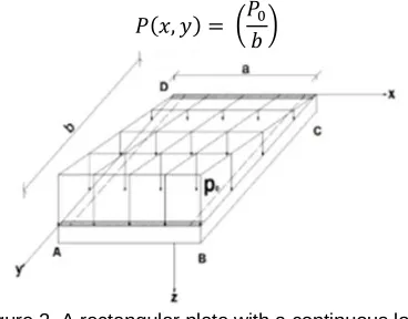
numerical deflection Mesh size - 4.803586254 0.503478 0.527663 10 - 3.09606378 0.503478 0.519066 12 - 2.039413837 0.503478 0.513746 14 - 1.661641621 0.503478 0.511844 16 - 1.202833093 0.503478 0.509534 20 - 0.875509953 0.503478 0.507886 24 - 0.745414894 0.503478 0.507231 26 - 0.632003782 0.503478 0.506659 28 - 0.532297341 0.503478 0.506158 30 - 0.443912147 0.503478 0.505713 32 - 0.365259257 0.503478 0.505317 34 - 0.294749721 0.503478 0.504962 36 - 0.173393872 0.503478 0.504351 40 - 0.120759993 0.503478 0.504056 42 - 0.072694338 0.503478 0.503844 44 - 0.050846313 0.503478 0.503734 46 - 0.052236642 0.503478 0.503741 48 - 0.049853221 0.503478 0.503729 50 - 0.037737498 0.503478 0.503669 54 - 0.018670131 0.503478 0.503572 58 - 0.0075475 0.503478 0.503516 60 - 0.004369605 0.503478 0.503453 62 - 0.016683946 0.503478 0.503394 64 - 0.029395525 0.503478 0.50333 66 - 0.055215918 0.503478 0.5032 70 - 0.085803153 0.503478 0.503046 78 - 0.083816969 0.503478 0.503056 80 - 0.090172758 0.503478 0.503024 90 - 0.11241802 0.503478 0.502912 100 - 0.124533743 0.503478 0.502851 120 - 0.14124769 0.503478 0.502757 140 - 0.145984532 0.503478 0.502746 160 - 0.148963808 0.503478 0.502728 180 - 0.155319597 0.503478 0.502696 200 - 0.159093347 0.503478 0.502677 250 100 Length (cm) 0.3 poisson's ratio 100 Width (cm) 10000
continuous load (kg/ m2)
1 Thickness (cm)
2400 Yeild Strenght (strain)
2100000
modulus of elasticity (kg/ cm2)
2400 Yeild Strenght
Two sides simply supported and two sides cantilever supported Support situation
266 Figure 3. Mesh sensitivity
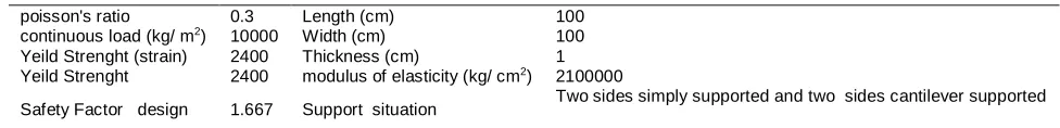
Figure 4. X- Axise normal stress countors (𝜎𝑥)
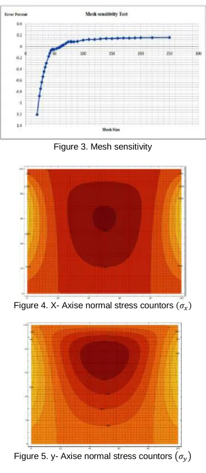
Figure 5. y- Axise normal stress countors (𝜎𝑦)
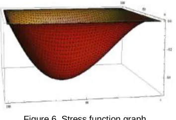
267 Figure 6. Stress function graph
CONCULSION
Given the difficulty and long analytical solution of the plate equations in some specific issues, using numerical methods is always a good practice, provided that the authenticity and accuracy of these methods can be evaluated and selecting optimized steps for iteration, both save time during the analysis of problems and get appropriate and acceptable accuracy. Finite difference method as one of the existing numerical methods is relatively strong method for numerical solution of the plate equations with different loading and support solutions conditions. As observed, increasing repeat steps in finite difference method does not result in increased attention to the problem and may also act in the opposite way.
REFERENCES
Boot JC and Moore DB. 1988. Stiffened plates subjected to transverse loadings, International Journal of Solids Structures, 24, 89-104.
Chakraborty R and Ghosh A. 2011. Finite difference method for computation of 1D pollutant migration through saturated homogeneous soil media, International Journal of Geomechanics,11, 12-22.
Kaiser R. 1936. Rechnerische und experimentelle ermittlung der durchbiegungen und spannugen von quadratischen platten bei freier auflagerung an den randern gleichmassig verteilter last und grussen ausbiegungen, ZFAMM, 16, 73-78.
Kan HP and Huang JC. 1967. Large deflection of rectangular sandwich plates, AIAA, 5, 1706-1708.
Kim CK. 2002. Iterative analysis of nonlinear laminated rectangular plates by finite difference method, Journal of the Korean Society of Safety, 10, 13-17.
Krysko V, Zhigalov M, Saltykova O and Krysko A. 2011. Effect of transverse shears on complex nonlinear vibrations of elastic beams, Journal of Applied Mechanics & Technical Physics, 52, 834-840.
Mochnacki B and Majchrzak E. 2010. Numerical modelling of casting solidification using generalized finite difference method, Materials Science Forum, 638, 2676-2681.
Rasmassen K, Burns T, Bezkorovaniny P and Bambach MR. 2003. Numerical modelling of anisotropic stainless steel plates, Journal of Contruction and Steel Res., 59, 1345-1362.
Tsui TY and Tong P. 1971. Satability of transient solution of moderately thich plate by finite difference method, Journal of the American Institute for Aeronautics and Astronautics, 9, 2062-2063.
Vallabhan CV. 1983. Iterative of nonlinear glass plates, Journal of Structural Engineering, ASCE,109, 1003-1017.
Wang Y, Wu W and Agarwal RP. 2011. A fourth-oder compact finite difference method for nonlinear higher-order multipoint boundary value poblems, Computers & Mathematics with Applications, 61, 3226-3245.
Wan Y. 2011. A modified accelerated monotone method for finite difference reaction-diffusion-convection equations, Journal of Computational & Applied Mathematics, 235, 3646-3660.
Wu W, Shu C, Xiang Y and Wang C. 2010. Free vibration and buckling analysis of highly skewed plates by least squares based finite difference method, Interna tional Journal of Structural Stability & Dynamics,10, 225-250.
Zhang S and Wang W. 2010. stencil of the finite difference for the 2D convection diffusion equation and its new iterative scheme, International Journal of Computer mathematics, 87, 2588-2600.