Estimating Corroded Area of Metallic Surfaces Using Edge Detection & Hole Filling

ISSN: 2231-5381

http://www.ijettjournal.org

Page 529

Estimating Corroded Area of Metallic Surfaces

Using Edge Detection & Hole Filling

Rajiv Kumar#1, Maninder Pal*2, Tarun Gulati#3

#1

M.Tech Scholar, #3Associate Professor, Department of Electronics & Communication Engineering, Maharishi Markandeshwar University, Mullana, Ambala, Haryana, INDIA

*2

Research Associate, NIBEC, University of Ulster, Jordanstown, Northern Ireland, UK

Abstract

—

Keywords - Corrosion Detection; Corrosion Estimation; Dilation; Erosion and Hole Filling

.

I. INTRODUCTION

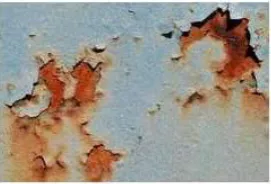
This paper focuses on developing a method for detecting and estimating the corroded area in an image of corroded metallic surface. A typical example of the corroded metallic surface is shown in Figure 1, in which the corroded surface shows both a color and contrast difference compared to the corresponding metallic surface. In image processing, this variation can be detected using edge detection [1-6]. When applied the same technique to the image of corroded metallic surfaces, it will result into corroded and non-corroded regions. These regions cover the entire image; with each region corresponding to some characteristic or property such as color, intensity or texture that defines corroded and non-corroded regions of the image. This image based analysis is a form of non-destructive testing and is expected to give far greater reproducible performance in comparison with visual inspection techniques done by humans. Therefore, this paper develops a system to detect and estimate the area of corroded metallic surface using edge detection.

Fig 1: Example of a corroded metal surface.

II. METHODOLOGY

The methodology used in this paper for partitioning the digital image of corroded metallic objects into corroded and non-corroded regions, is mentioned below.

--- 1. Read and scale the image.

2. Detect the corroded surface using the edge detection. 3. Dilate the detected surface image.

4. Fill the interior gaps between the detected surface regions using hole filling.

5. Remove connected objects on border. 6. Smoothening the image.

7. Calculation of parameters (area) of the detected region. --- The key steps involved are discussed below.

A. Edge detection

ISSN: 2231-5381

http://www.ijettjournal.org

Page 530

There is large number of edge detection operators available, each designed to be sensitive to certain types of edges; however, the key edge detection methods are:

1) Gradient: The gradient method detects the edges by looking for the maximum and minimum in the first derivative of the image.

2) Laplacian: The Laplacian method searches for zero

crossings in the second derivative of the image to find edges. An edge has the one-dimensional shape of a ramp and calculating the derivative of the image can highlight its location. This method of locating an edge is characteristic of the “gradient filter” family of edge detection filters and also includes the Sobel method [15-17]. A pixel location is declared an edge location, if the value of the gradient exceeds some threshold. Edges have higher pixel intensity values than those surrounding it; however, once a threshold is set, the gradient value to the threshold value can be compared and an edge can be detected whenever the threshold is exceeded. Furthermore, when the first derivative is at a maximum, the second derivative is zero. As a result, another alternative to finding the location of an edge is to locate zeros in the second derivative.

3) Sobel operator: The Sobel operator consists of a pair of 3×3 convolution kernels as shown in Table 1. One kernel is simply the other rotated by 90°. These kernels are designed to respond maximally to edges running vertically and horizontally relative to the pixel grid, one kernel for each of the two perpendicular orientations [15-24]. The kernels can be applied separately to the input image, to produce separate measurements of the gradient component in each orientation (Gx and Gy). These can then be combined together to find the absolute magnitude of the gradient at each point and the orientation of that gradient. The gradient magnitude is given by:

| | √ (1)

Typically, an approximate magnitude is computed using:

| | | | | | (2)

Table 1: Masks used by Sobel operator.

-1 0 +1 +1 +2 +1

-2 0 +2 0 0 0

-1 0 +1 -1 -2 -1

Gx Gy

4) Canny: This method was proposed by John F. Canny in 1986. Canny operator uses templates of different directions to do convolution to the image respectively [24-29]. The Canny operator edge detection is to search for the partial maximum value of image gradient. The gradient is counted by the derivative of Gaussian filter. The Canny operator uses two thresholds to detect strong edge and weak edge respectively. The gradient magnitude and direction is calculated using first order finite differences. The second criterion is that the edge points be well localized. In other words, the distance between the edge pixels as found by the detector and the actual edge is to be at a minimum. A third criterion is to have only one response to a single edge. This was implemented because the

first two were not substantial enough to completely eliminate the possibility of multiple responses to an edge. More specifically, the Canny edge detector firstly smoothes the image to eliminate noise. It then finds the image gradient to highlight regions with high spatial derivatives. The algorithm then tracks along these regions and suppresses any pixel that is not at the maximum (non-maximum suppression). The gradient array is then further reduced by hysteresis. Hysteresis is used to track along the remaining pixels that have not been suppressed. Hysteresis uses two thresholds and if the magnitude is below the first threshold, it is set to zero (made a non-edge). If the magnitude is above the high threshold, it is made an edge. And if the magnitude is between the 2 thresholds, then it is set to zero unless there is a path from this pixel to a pixel with a gradient above threshold 2. The main advantage of this method is elimination of multiple responses to a single edge. It also have a good localization property, means the detected edges are much closer to the real edges.

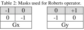
5) Robert’s cross operator: The Roberts cross operator performs a simple, quick to compute, 2-D spatial gradient measurement on an image [24-29]. Pixel values at each point in the output represent the estimated absolute magnitude of the spatial gradient of the input image at that point. The operator consists of a pair of 2×2 convolution kernels as shown in Table 2. One kernel is simply the other rotated by 90°. This is very similar to the Sobel operator. These kernels are designed to respond maximally to edges running at 45° to the pixel grid, one kernel for each of the two perpendicular orientations. The kernels can be applied separately to the input image, to produce separate measurements of the gradient component in each orientation (Gx and Gy).

Table 2:Masks used for Roberts operator.

These can then be combined together to find the absolute magnitude of the gradient at each point and the orientation of that gradient. The gradient magnitude is given by:

|G| = |Gx| + |Gy| (3)

6) Prewitt’s operator: Prewitt operator is similar to the Sobel operator with a slight variation in the mask coefficients (Table 3) and is used for detecting vertical and horizontal edges in images [15-24].

Table 3: Masks used for Prewitt’s operator.

-1 0 +1 +1 +1 +1

-1 0 +1 0 0 0

-1 0 +1 -1 -1 -1

Gx Gy

7) Proposed edge detection algorithm for detecting corroded surfaces: The edge detection algorithm proposed for the purpose of detecting the edges of corroded region in an image of corroded metallic surface is mentioned below. ---

-1 0 0 +1

0 -1 -1 0

ISSN: 2231-5381

http://www.ijettjournal.org

Page 531

1. Read Image and consider A be an image matrix and B be a structuring element.

2. Scale the image.

3. Threshold the images. (Compute the maximum and minimum value of the pixel in the image. Compute the average and compare the values of each pixel with the threshold).

4. Mark the initial set of edges and then take the invert of edges.

5. Convert the edges to squares based structuring elements using erosion.

6. Subtract the binary image A from the eroded image to get the final edges as:

( ) ( ) (4)

---

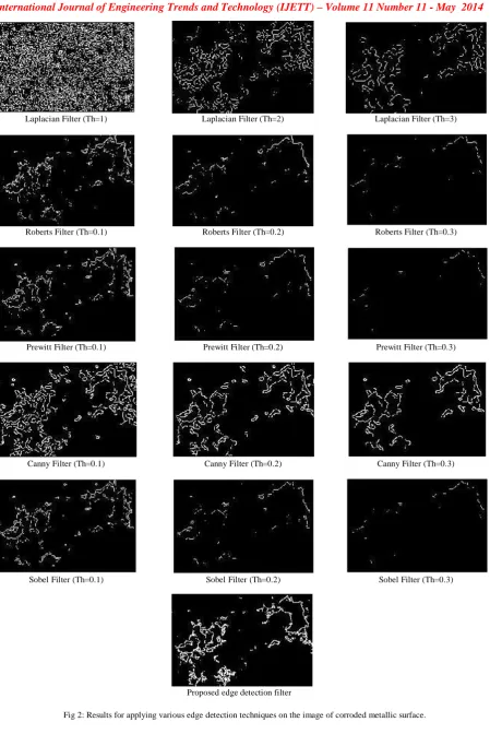
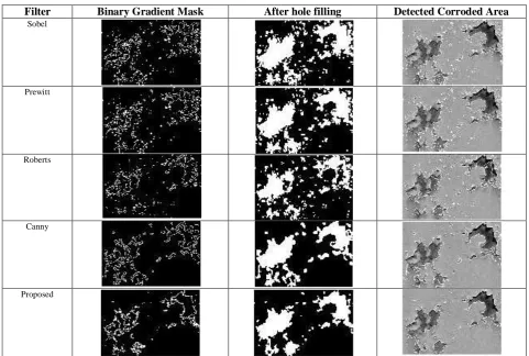
The results (when applied on an image of corroded surface) obtained for the above mentioned algorithms are shown in Figure 2. The Laplacian filter shows high noise; and thus false edges at lower threshold value of 1; and with increase in threshold, it misses the true edges. Thus, it is not found suitable for the purpose of detecting corrosion on metallic surfaces. The gradient-based algorithms (Roberts and Perwitt filter) is also not found suitable (Figure 2), as these also have a major drawback of being highly sensitive to noise. It is also because, the size of the kernel filter and coefficients are fixed and cannot be adapted to a given image. The Canny edge detection algorithm performs better than all the mentioned operators. This was expected as Canny edge detection accounts for regions in an image. However, Canny’s edge detection algorithm is computationally more expensive compared to Sobel, Prewitt and Robert’s operator. It is also observed from visual results that none of the mentioned algorithms is able to preciously locate the edges in the images of corroded metallic surfaces. The results obtained for the proposed algorithm (Figure 2) clearly shows better performance over the mentioned algorithms.

B. Dilation & Erosion of the Image

Dilation and erosion are the two basic operators in the area of mathematical morphology. These are usually applied to binary images. The basic effect of the dilation operator on a binary image is to gradually enlarge the boundaries of regions of foreground pixels (i.e. white pixels). Thus, areas of foreground pixels will grow in size while holes within those regions become smaller. However, the basic effect of the erosion operator on a binary image is to erode away the boundaries of regions of foreground pixels (i.e. white pixels, typically). This means the area of foreground pixels will shrink in size, and holes within those areas become larger. Both the dilation and erosion operator takes two pieces of data as inputs. The first is the image to be dilated or eroded. The second is a (usually small) set of coordinate points known as structuring element (also known as kernel). It is this structuring element that determines the precise effect of the dilation/erosion on the input image. The mathematical

definition of dilation and erosion for binary images is as follows:

Suppose that X is the set of Euclidean coordinates corresponding to the input binary image, and that K is the set of coordinates for the structuring element. Let Kx denote the translation of K so that its origin is at x. Then the dilation and erosion of X by K is simply the set of all points x such that the intersection of Kx with X is non-empty and Kx is a subset of X

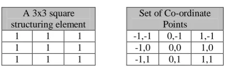
respectively. An example of structuring element of 3×3 square, with the origin at its center, as shown in Table 4. It is to be noted that the foreground pixels are represented by 1's and background pixels by 0's.

Table 4: A 3x3 square structuring element.

A 3x3 square structuring element

Set of Co-ordinate Points

1 1 1 -1,-1 0,-1 1,-1

1 1 1 -1,0 0,0 1,0

1 1 1 -1,1 0,1 1,1

To compute the dilation of a binary input image by this structuring element, firstly each of the background pixels in the input image in turn is considered. For each background pixel (which is called the input pixel), the structuring element is superimposed on top of the input image so that the origin of the structuring element coincides with the input pixel position. If at least one pixel in the structuring element coincides with a foreground pixel in the image underneath, then the input pixel is set to the foreground value. If all the corresponding pixels in the image are background; then, the input pixel is left at the background value.

ISSN: 2231-5381

http://www.ijettjournal.org

Page 532

Laplacian Filter (Th=1) Laplacian Filter (Th=2) Laplacian Filter (Th=3)

Roberts Filter (Th=0.1) Roberts Filter (Th=0.2) Roberts Filter (Th=0.3)

Prewitt Filter (Th=0.1) Prewitt Filter (Th=0.2) Prewitt Filter (Th=0.3)

Canny Filter (Th=0.1) Canny Filter (Th=0.2) Canny Filter (Th=0.3)

Sobel Filter (Th=0.1) Sobel Filter (Th=0.2) Sobel Filter (Th=0.3)

Proposed edge detection filter

ISSN: 2231-5381

http://www.ijettjournal.org

Page 533

(a) Input Image (b) Dilated Image (c) Eroded Image

Fig 3: Effect of dilation & erosion using a 3×3 square structuring element.

C. Hole filling

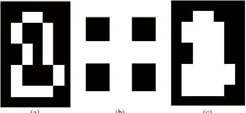
To understand the concept of hole filling, consider the binary image (Figure 4) which has a background and foreground. Foreground is nothing more than a boundary of 1′s surrounded by 0′s background pixels.

(a) (b) (c)

Fig 4: (a) Input image, (b) mask and (c) output image filled with holes.

The ‘1’ shaped image in Figure 4(a) can be filled using the following steps:

1) Identifying the location of a pixel bounded within boundary of foreground pixels (i.e location of a pixel within area to be filled).

2) Perform dilation of that pixel with a mask shown in Figure 4b. After performing dilation, the result’s intersection

with original image’s compliment is taken. After each successive iteration, the input is filled with foreground pixels. This process is repeated until no further changes occur, i.e., all holes are filled. Finally, in order to make the segmented object look natural, the object is smoothened by eroding the image twice with a diamond structuring element. The diamond structuring element is created using the strel function of Matlab. The area of this smoothed object (corroded region) is then calculated by calculating the total number of pixels.

III. RESULTS&DISCUSSION

The algorithm presented to detect the corroded region in a metallic surface and to estimate the corroded area is implemented in Matlab. The developed algorithm is tested for several images; however for simplicity, the results obtained

for few are mentioned in this paper. In particularly, the results obtained are divided into the following three parts:

1. The first part discusses the efficiency of the proposed edge detection algorithm based on morphological erosion operation.

2. The second part investigates the accuracy of the proposed corrosion based algorithm on the images of objects with known area.

3. In the third part, the corrosion detection algorithm is tested for various real pictures of corroded surfaces. The results obtained for the above three cases is discussed below.

Case I: Investigating the efficiency of the proposed edge detection algorithm

ISSN: 2231-5381

http://www.ijettjournal.org

Page 534

Filter Binary Gradient Mask After hole filling Detected Corroded Area

Sobel

Prewitt

Roberts

Canny

Proposed

Fig 5: Results of applying the proposed corrosion detection algorithm using various edge detection algorithms.

Case II: The second part investigate the accuracy of the proposed corrosion based algorithm for the images of objects with known area. To better investigate the accuracy of the proposed corrosion detection algorithm, three images of rectangle, circle and triangle are taken, as shown in Figure 6. The benefit of taking these shapes is that it helps understanding the effects of lines, curves and corners. A maximum error of 1.124% (Table 5) in the estimated area is noted which is considered low in practice. Therefore, the combination of the proposed corrosion detection algorithm along with the proposed edge detection algorithm is found suitable for detecting and estimating the area of corroded region in the image of corroded metallic surface.

Table 5: Estimated corroded surface.

Picture Estimated Corroded

Area (%)

Error (%)

18.8297% 0.652%

26.7896% 0.542%

33.0468% 1.124%

Input Image Dilated Gradient Mask After Filling Holes Outlined Original Image

Fig 6: Results of applying the proposed corrosion detection algorithm using proposed morphology based edge detection on an image of rectangle, circle and triangle. The images shown are reduced to 20% to their original because of restricted space.

ISSN: 2231-5381

http://www.ijettjournal.org

Page 535

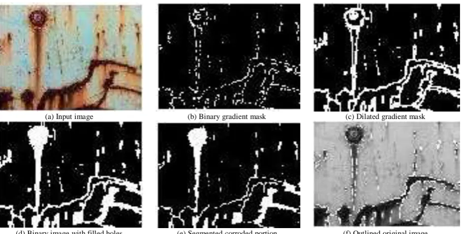
In the third part, the corrosion detection algorithm is tested for various real pictures of the corroded metallic surfaces. The results obtained are shown in Figures 7 and 8. From the visual inspection of the results, it is observed that the proposed algorithm has given satisfactory repeatable performance in

detecting the corroded region. This confirms the suitability of the proposed algorithm for real time applications.

(a) Input image (b) Binary gradient mask (c) Dilated gradient mask

(d) Binary image with filled holes (e) Segmented corroded portion (f) Outlined original image Fig 7: Results of applying the proposed corrosion detection algorithm on a real picture of corroded surface 1.

Estimated corroded area in percentage is 20.7305%.

(a) Input image (b) Binary gradient mask (c) Dilated gradient mask

(d) Binary image with filled holes (e) Segmented corroded portion (f) Outlined original image Fig 8: Results of applying the proposed corrosion detection algorithm on a real picture of corroded surface 2.

ISSN: 2231-5381

http://www.ijettjournal.org

Page 536

IV.CONCLUSIONS

This paper presented the results obtained for the algorithm to identify the corroded and non-corroded regions in an image of a metallic corroded surface. This image based analysis is a form of non-destructive testing. The developed algorithm is tested for several images; and the results obtained are divided into three parts. The first part discusses the efficiency of the proposed edge detection algorithm based on morphological erosion operation. In this case, the proposed edge detection algorithm is tested for detecting the corroded area in images of the corroded surfaces. The algorithm is tested in comparison with famous Sobel, Prewitt, Roberts and Canny algorithms. From the results obtained, it is found to be able to detect the corroded surface even in high color/contrast variation of corroded surface. The second part investigates the accuracy of the proposed corrosion based algorithm on the images of objects with known area. For this purpose, three images of rectangle, circle and triangle are taken. The benefit of taking these shapes is that it helps understanding the effects of lines, curves and corners. In the third part, the corrosion detection algorithm is tested for various real pictures of corroded surfaces. From the visual inspection of the results, it is observed that the proposed algorithm has given satisfactory performance in detecting the corroded region. This confirms the suitability of the proposed algorithm for real time applications. Thus, the combination of the proposed corrosion detection algorithm along with the proposed edge detection algorithm is found suitable for detecting and estimating the area of corroded region in the image of corroded metallic surface.

V. REFERENCES

[1] M. H. Olyaee, H. Abasi and M. Yaghoobi (2013), “Using Hierarchical Adaptive Neuro Fuzzy Systems And Design Two New Edge Detectors In Noisy Images”, Journal of Soft Computing and Applications, vol. 2013, pp. 1-10.

[2] Patricia Melin, Claudia I. Gonzalez, Juan R. Castro, Olivia Mendoza and Oscar Castillo (2013), “Edge Detection Method for Image Processing based on Generalized Type-2 Fuzzy Logic”, IEEE Transactions on Fuzzy Systems TFS-2013-0313.R21.

[3] Hankyu Moon, Rama Chellappa, and Azriel Rosenfeld (2012), “Optimal Edge-Based Shape Detection”, IEEE transactions on image processing, Vol. 11, No. 11, Nov. 2012.

[4] S. Sathish Kumar and R. Amutha (2012), “Edge Detection of Angiogram Images Using the Classical Image Processing Techniques”, IEEE-International Conference On Advances In Engineering, Science And Management (ICAESM -2012) March 30- 31, 2012.

[5] Johannes Jordan and Elli Angelopoulou (2011), “EDGE Detection In Multispectral Images Using The N-Dimensional Self-Organizing Map”, 18th IEEE International Conference on Image Processing Brussels, 11-14 Sept. 2011, pp. 3181 – 3184.

[6] Carlos G. Spinola, Juan Canero, Gonzalo Moreno-Aranda, Jose M.Bonelo, Manuel. Martin-Vazquez1 (2011), “Real-Time Image Processing for Edge Inspection and Defect Detection in Stainless Steel Production Lines”, IEEE International Conference on Imaging Systems and Techniques (IST), Penang, pp. 170-175, 2011. [7] Nicolas Widynski and Max Mignotte (2011), “A Contrario Edge

Detection with Edgelets”, 2011 IEEE International Conference on Signal and Image Processing Applications (ICSIPA-2011). [8] You-yi Zheng, Ji-lai Rao and Lei Wu (2010), “Edge Detection

Methods in Digital Image Processing”, The 5th International

Conference on Computer Science & Education Hefei, China. August 24–27, 2010.

[9] Zhang Jin-Yu, Chen Yan and Huang Xian-Xiang (2009), “Edge Detection of Images Based on Improved Sobel Operator and Genetic Algorithms”, IASP 2009, International Conference on Image Analysis and Signal Processing, Taizhou, 2009.

[10] Feng-ying Cui and Li-jun Zou Bei Song (2008), “Edge Feature Extraction Based on Digital Image Processing Techniques”, Proceedings of the IEEE International Conference on Automation and Logistics Qingdao, China, September 2008.

[11] C. Kang, and W. Wang (2007), “A novel edge detection method based on the maximizing objective function”, Elsevier Journal of Pattern Recognition, Vol. 40, pp. 609 – 618.

[12] Y. Yu, C. Chang (2006), “A new edge detection approach based on image context analysis”, Elsevier Journal of Image and Vision Computing, Vol. 24, pp. 1090–1102.

[13] A. Koschan and M. Abidi (2005), “Detection and Classification of Edge Color Images”, IEEE Signal Processing Magazine, pp 64-73, January 2005.

[14] S. Konishi, A. L. Yuille, J. M. Coughlan and S. C. Zhu (2003), “Statistical Edge Detection: Learning and Evaluating Edge Cues”, IEEE Transactions On Pattern Analysis And Machine Intelligence, Vol. 25, No. 1, pp 57-74.

[15] A. D. Santis and C. Sinisgalli (1999), “A Bayesian Approach to Edge Detection in Noisy Images”, IEEE Transactions On Circuits And Systems—I: Fundamental Theory And Applications, Vol. 46, No. 6, pp 686-699.

[16] J. C. Bezdek, R. Chandrasekhar, and Y. Attikiouzel (1998), “A Geometric Approach to Edge Detection”, IEEE Transactions On Fuzzy Systems, Vol. 6, No. 1, pp 52-75.

[17] G. Deng and L.W. Cahill (1994), “An adaptive Gaussian filter for noise reduction and edge detection”, in Proceedings of IEEE Science Symposium on Medical Imaging, pp. 1615–1619.

[18] H. Jeong and C. I. Kim (1992), “Adaptive determination of filter scales for edge-detection”, IEEE Transactions on Pattern Analysis and Machine Intelligence, Vol. 14, pp. 579–585.

[19] J. D. Scargle and M. K. Quweider (1991), “Edge Detection Using Dynamic Optimal Partitioning”, Pattern Recognition, Vol. 24(6), pp. 465-478.

[20] P. Perona and J. Malik (1990), “Scale-space and edge detection using anisotropic diffusion”, IEEE Trans. Pattern Anal. Machine Intell., Vol. 12, pp. 629–639, July 1990.

[21] V. Lacroix (1990), “The primary raster: A multiresolution image description”, in Proc. 10th Int. Conf. Pattern Recognition, 1990, pp. 903–907.

[22] D. J. Williams and M. Shah (1990), “Edge contours using multiple scales”, Computing Visual Graph Image Processing, Vol. 51, pp. 256–274, 1990.

[23] B. G. Schunck (1987), “Edge detection with Gaussian filters at multiple scales”, in Proc. IEEE Comp. Soc. Work. Comp. Vis., 1987, pp. 208–210.

[24] J. Canny (1986), “A Computational Approach to Edge Detection”, IEEE Transaction on Pattern Analysis and Machine Intelligence, Vol. 6, pp. 679-698.

[25] A. L. Yuille and T. A. Poggio (1986), “Scaling theorems for zero-crossings”, IEEE Transactions on Pattern Analysis and Machine Intelligence, Vol. PAMI-8, pp. 15–25.

[26] G. Giraudon (1985), “Edge Detection from Local Negative Maximum of Second Derivative”, In Proceedings of IEEE, International Conference on Computer Vision and Pattern Recognition, pp. 643-645.

[27] R. M. Haralick (1984), “Digital step edges from zero-crossing of second directional derivatives”, IEEE Trans. Pattern Analysis and Machine Intelligence, Vol. PAMI-6, pp. 58–68.

[28] J. Canny (1983), “Finding Edges and Lines”, MIT Technical Report No. 720, 1983.

[29] R.M. Haralick (1983), “Ridge and Valley on Digital Images”,