Compressive sampling based CFO estimation with exploited features

R E S E A R C H

Open Access

Compressive sampling-based

CFO-estimation with exploited features

Chaojin Qing

, Jiafan Wang

, Chuan Huang

and Hongyuan Chen

Abstract

Based on the compressed sensing (CS) technique, the carrier frequency offset (CFO) is estimated in compressive sampling scenarios. We firstly confirm the compressibility of estimation metric vector (EMV) of conventional maximum likelihood (ML)-based CFO estimation, and thus conduct the compressive sampling at receiver. By exploiting the EMV features, introducing a circle cluster, and proposing a novel coherence-pattern, we then form a feature-aided weight coherence (FAWC) optimization to optimize measurement-matrix. Besides the proposed FAWC optimization, by referencing compressive sampling matching pursuit (CoSaMP) algorithm and exploiting EMV features, a metric-feature based CoSaMP (MFB-CoSaMP) algorithm is proposed to improve the EMV-reconstruction accuracy, and to reduce computational complexity of classic CoSaMP. With reconstructed EMV, we finally develop a CFO estimation method to estimate the coarse CFO and fine CFO. Relative to weighted coherence minimization (WCM) and classic CoSaMP, the elaborate performance evaluations show that the FAWC and MFB-CoSaMP can independently or jointly improve accuracy of the CFO-estimation (including coarse CFO-estimation and fine

CFO-estimation), and the improvement is robust to system parameters, e.g., sparsity level, number of measurements, etc. Furthermore, the mean squared error (MSE) of proposed CFO estimation method can almost reach to its Cramer-Rao lower Bound (CRLB) when a relative large number of measurements, a relative high carrier-to-noise ratio´ (CNR), and a reasonable length of observed signals can be obtained.

Keywords: Carrier frequency offset, Compressed sensing, Estimation metric, CoSaMP, Equivalent Likelihood function

1 Introduction

The carrier frequency offset (CFO), which is one of the well understood radio frequency (RF) impairment, may result in severe performance degradation at the receiver [1, 2]. To improve receiver performance, the CFO estima-tion has been studied comprehensively. In [3–5], the CFO estimations for additive white Gaussian noise (AWGN) channels, flat fading channels and frequency-selective fading channels are respectively addressed. Recently, the proposed compressive sensing (CS) approach [6, 7], which enables sub-Nyquist sampling of sparse or compressible signals in some domain, can be employed to reduce sys-tem complexity and to save power significantly. By exploit-ing the sparsity profile, the CS-based CFO estimation is presented in [8, 9] for multi-user uplink. Compared with the CFO estimation without utilizing CS, the estimation

*Correspondence: [email protected]

1_{School of Electrical Engineering and Electronic Information, Xihua University,} 610039 Chengdu, China

Full list of author information is available at the end of the article

accuracy is improved due to the priori information of sparse approximation. Although various methods of CFO estimation are proposed with and without utilizing CS, the sampling rate of these existing methods for CFO estima-tion, e.g., [3–5, 8, 9], needs to be at least the Nyquist rate, resulting in excessive power consumption and design dif-ficulty for the analog-to-digital converter (ADC) when the high sampling rate is experienced [10, 11].

To reduce the sampling rate, the CS is introduced into synchronization issue in [12–14]. In [12], a fast and rough estimate of pseudo-noise (PN) code phase and Doppler frequency with a reduced number of parallel correla-tors (i.e., compressed correlacorrela-tors) is proposed, where the sparse expression is based on autocorrelation. For binary phase-shift keying (BPSK) signals and binary offset carrier (BOC) modulation signals, the 2-D compressed correla-tor (TDCC) technique for the rough estimate of PN code phase and Doppler frequency is introduced in [13, 14], respectively. Based on hypothesis testing for a code phase

and Doppler frequency next to the true hypothesis can yield a non-negligible amount of signal energy, the pressed correlators technique in [12–14] tests a com-pressed hypothesis and coherently combines the signal energy in the neighboring hypotheses. Although the num-ber of correlators is reduced, the compressed correlator technique can only roughly estimate Doppler frequency. Furthermore, the features of estimation metric vector (EMV) of CFO estimation are not exploited for com-pressive sampling and signal reconstruction. Thus, the CS-based CFO estimation, which includes coarse estima-tion and fine estimaestima-tion, is not intensively investigated in [12–14].

By exploiting the features of EMV, a novel CS-based CFO estimation is proposed in this paper. The com-pressive sampling is introduced into Maximum Likeli-hood (ML)-Based CFO estimation to reduce sampling rate while holding estimation performance be not deteriorated significantly. We briefly describe some critical points of the proposed CS-based CFO estimation as the follows.

• Feasibility analysis of compressive sampling:

Based on the compressibility of EMV in ML-based CFO estimation [15], we first verify the received signal can be obtained with compressive sampling, and the ADC requirement can be reduced.

• Optimization of measurement matrix:In compressive sampling, measurement matrix directly determines whether the reconstruction can be realized successfully [6, 7]. The designing of efficient measurement matrices becomes the core problem for higher probability of reconstruction. In [16], Baraniuk et al. have been proved that many random matrices are good measurement matrices, and some optimized methods can also be found in existing literatures, such as [17–22]. These existing methods, however, are not specially designed for CFO estimation, and thus cannot obtain an optimized performance (e.g., reconstruction-accuracy improvement for EMV recovery). To obtain a more suitable measurement matrix, we exploit the features of EMV. Firstly, the

EMV is expressed as acircle cluster to reduce the

block-sparsity to one (i.e., significant amplitudes are gathered in one sub-block when EMV is divided into multiple sub-blocks). With the special structure of block-sparsity, a novel coherence-pattern is proposed to fully utilize structure information of circle cluster. Then, a feature-aided weight coherence (FAWC) optimization, based on the algorithm of weighted coherence minimization (WCM) [22], is developed to optimize measurement-matrix without

computational complexity increasing.

• Reconstruction algorithm:The reconstruction algorithm is another critical factor for successful

reconstruction. With the compressive sampling at receiver, many recovery algorithms are proposed. Among these reconstruction algorithms, we mainly reference the compressive sampling matching pursuit (CoSaMP) [23, 24], due to its high

reconstruction accuracy and excellent robustness to noise. According to the CoSaMP algorithm and the EMV features, a metric feature-based CoSaMP (MFB-CoSaMP) algorithm is proposed to improve the EMV reconstruction accuracy, and to reduce the computational complexity of classic CoSaMP.

• CFO estimation:With the reconstructed EMV, we implement the CFO estimation by using a two-step procedure which includes coarse and fine CFO estimation. In the coarse of CFO estimation, the likelihood function is constructed according to EMV and to seek the local maximum. As for the fine CFO estimation, the received signal vector is recovered at Nyquist rate with the reconstructed EMV and then used to generate the likelihood function, with which an interpolation method is employed to seek the local maximum near to the value of coarse CFO estimation.

Performance evaluation shows that the proposed CS-based CFO estimation can be implemented with reduced sampling-rate, along with an acceptable esti-mation deterioration in terms of mean squared error (MSE). Compared with the optimization of weighted coherence minimization (WCM) [22] and the recon-struction algorithm CoSaMP, the elaborate performance evaluations present the proposed FAWC and MFB-CoSaMP can independently or jointly improve the accuracy of estimation (including coarse CFO-estimation and fine CFO-CFO-estimation), and the improve-ment is robust to system parameters, e.g., the sparsity level, the number of measurement, and the length of the observed signal. Furthermore, the MSE of proposed CFO-estimation can almost reach to its Crame´r-Rao lower bound (CRLB) when the reasonable conditions can be obtained.

The main contributions of this paper are summarized as follows.

(a) We confirm the compressibility of CFO EMV in conventional maximum likelihood (ML)-based CFO estimation. Thus, the compressive sampling can be employed for CFO estimation.

method is robust to the designed parameters, and can easily to reach its convergence.

(c) An MFB-CoSaMP algorithm is proposed to reconstruct EMV by exploiting its features. Compared with the classic CoSaMP algorithm, the proposed method improves the recovery accuracy and reduces the computational complexity.

Furthermore, the improvement of recovery-accuracy is robust against to the varying of parameters. (d) We implement the CFO estimation (including coarse

and fine estimation) with compressive sampling. Furthermore, the MSE performance can reach to its CRLB when reasonable system parameters are obtained.

The rest of this paper is organized as follows. In Section 2, we formulate the method of compressive sampling for CFO estimation, where the expression of sampling is derived from the ML-based approach in a conventional system model of Nyquist rate. Section 3 deals with the optimization of measurement matrix by exploiting EMV features. In Section 4, the CFO esti-mation method is proposed, where we present the MFB-CoSaMP recovery-method, coarse CFO estimation, and fine CFO estimation. Performance evaluations are shown in Section 5. Finally, Section 6 concludes this paper.

Notation: We use boldface letters to denote matrices and column vectors;0denotes the zero vector of arbitrary size; (·)T_,(·)H_,(·)−1_,(·)†_{, and·, denote the transpose,}

con-jugate transpose, matrix inversion, Moore-Penrose matrix inversion, and floor operation, respectively; IP is P × P identity matrix; G(i,j) is the (i,j)th element of the matrix ofG; we write·_pfor the usualpvector norm: xp =

xp_i1/p; supp(x) = {i:xi=0} is the sup-port set that denotes the index set of nonzero elements inx;T denotes the column sub-matrix comprising the T columns of;x|T denotes the entries of the vectorx in the setT; the complementary set of setT is denoted by Tc, Ø denotes empty set, andE{·}is the expectation operator.

2 Compressive sampling for CFO estimation According to the conventional ML-based CFO estima-tion, we verify the feasibility of compressive sampling for CFO estimation in this section. In Subsection 2.1, We briefly describe the method of conventional ML-based CFO estimation. Then, in Subsection 2.2, we raise the compressible EMV, and summarize its features. Based on the compressibility of EMV, the feasibility of compressive sampling for CFO-estimation is verified in Subsection 2.3, according to the derivation result that the received signals (not EMV) can directly conduct compressive sampling.

2.1 Conventional ML-based CFO estimation

From [15], without compressive sampling, the observation of the sampled signal can be expressed as

rk=ej(2πfkTs+θ)+vk, 1≤k≤N, (1)

where f is the frequency offset to be estimated, Ts ≤ 1/2·fis the sampling interval,θ is an unknown ran-dom phase with uniform probability density in [ 0, 2π), and v_k is a sample of the complex AWGN with zero mean and varianceσ2_{. The carrier-to-noise ratio (CNR)}

ρ, which is the ratio of the signal to noise powers in (1), is defined as [15]

ρ= 1

2σ2. (2)

In the conventional estimation method [15], the prob-lem of ML estimation of the frequencyf is to seek the maximum of the equivalent likelihood function

f=N i=1rie

−j2πf·iTs 2

= N k=1

N

m=1rkr ∗ me−j2π

_{f Ts(k−m)} ,

(3)

wheref is a tentative value forf.

2.2 Sparsity of CFO EMV

Assume f=N i=1rie

−j2πf·iTs_{, then the vector form}

of fcan be expressed as

f

=rT·

f

, (4)

whererand

f

are, respectively,

r=[r1,r2,· · ·,rN]T, (5)

and

f= e−j2πf·Ts_,· · ·_,e−j2πf·NTsT_{. (6)}

In this paper, we name

f

asCFO estimation met-ric (EM). From (3), the equivalent likelihood function fcan be rewritten as

f= f2=rT·

f2. (7)

For grid search, P (P ≥ N) tentative values of f, denoted asf1,f2,· · ·,fP, are considered. For simplic-ity, we consider P = N in this paper due to the same conclusions. According to thePtentative values, we form an EMV (denoted by) as

= f1

, f2

,· · ·, fP

T

Substituting fp

In (8), the EMV is approximately sparse. That is, for the element-amplitudes of EMV (i.e.,

f1,· · ·,

fP), only a few amplitudes are significant and the rest are nearly zero or negligible.

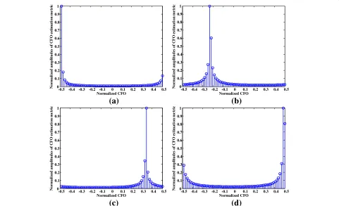
The examples are given in Fig. 1 to illustrate the com-pressibility of EMV, whereN = 64,P = 64,Ts = 10−9s,

f.Ts ∈ (−0.5, 0.5) is the normalized CFO. Note that we just consider the noise-free case in order to reveal the CFO features obviously. Four cases of normalized CFO, i.e.,f.Ts = −0.4976 (near to−0.5),f.Ts = −0.2441 (between−0.5 and 0),f.Ts = 0.3241 (between 0 and 0.5), andf.Ts=0.4757 (near to 0.5), are given in (a)−(d), respectively. From (a)−(d) in Fig. 1, and a large number of other experiments, theintrinsic featuresof EMV could be summarized as follows.

(a) Only a few element-amplitudes in EMV are significant.

(b) The significant amplitudes only gather in one cluster when the normalized CFOs connect to a circle from

−0.5to 0.5. In this paper, this cluster in a circle is

denominated ascircle cluster (i.e., significant

amplitudes form a cluster in a circle).

Note that the CFO estimation metrics are not in a clus-ter in a strict sense for the special case that the normalized CFOs are located near to −0.5 (or 0.5). When the nor-malized CFOs are located near to −0.5 (or 0.5), some significant amplitudes appear near to 0.5 (or−0.5). Thus, we still describe this feature as cluster due to its cycle periodicity when the normalized CFOs are connected from−0.5 to 0.5 to a circle. For convenience, we call this

-0.5 -0.4 -0.3 -0.2 -0.1 0 0.1 0.2 0.3 0.4 0.5

cluster in this paper as circle cluster, i.e., a cluster in a circle.

According to theintrinsic features, EMV can be com-pressed according to the comcom-pressed sensing theory [6, 7]. For expression convenience, we also call the intrin-sic featuresof EMV asEMV featuresin this paper.

2.3 Feasibility of compressive sampling for CFO

estimation

As verified in Subsection 2.1, the CFO EMV, i.e.,, can be compressed. However, the compressibility of CFO EMV

dose not mean that the received signalrcan conduct compressive sampling, for the reason that the sparsity lies in CFO EMVrather than the received signalr. Thus, we need to further analyze the compressibility of CFO EMV

and whether it could be mapped to the compressive sampling of the receive-signalr.

Based on the compressed sensing theory [6, 7], anM×P (MN≤P) measurement matrixcan be employed to compress the EMVdue to its sparsity. Then, anM×1 measurements, denoted asy, is given by

y=. (11)

Substituting=r(see (9)) into(11), we can derive

y=r=r, (12)

where theM×N matrix = is defined assensing matrix, and can be expressed as

=[1,2,· · ·,M]T, (13)

wherem=[θm1,θm2,· · ·,θmN]T, m=1, 2,· · ·,M. Fortunately, the derived expression in (12) can be directly employed to perform the compressive sampling of received signal r due to its form y = r. Note that, sinceMis significantly smaller thanN,y=rinfers that r (not EMV) can be compressed by theM×N matrix , i.e., the compressive sampling of received signalrcan be directly conducted. With the sensing matrix , we can adopt the generic circuit architecture of analog-to-information converter (AIC) [25] or modulated wideband converter (MWC) model [26] to implement compressive sampling. Due toM N, the sampling rate can be nat-urally reduced, i.e., the ADCs at sub-Nyquist rate can be employed for CFO estimation.

After conducting the compressive sampling according to (12), we will use reconstruction-approach to recon-struct the EMV and then perform the CFO estimation based on the reconstructed EMV. Especially, the recon-struction accuracy is mainly decided by the measure-ment matrix and reconstruction algorithms [6, 7]. Thus, we optimize the measurement-matrix in Section 3 and improve the reconstruction-algorithm in Section 4 for a better reconstruction-accuracy of EMV.

3 Optimization of measurement matrix

In CS theory, the measurement matrix plays an impor-tant role to determine the performance of reconstruction [6, 7], because a more efficient measurement matrix for the compressive sampling leads to the higher probabil-ity of reconstruction. In [16], Baraniuk et al. have been proved that many random matrices are good measure-ment matrices. The optimized methods can be found in [17–22]. However, these existing methods are not specially designed for CFO estimation. Thus, the EMV features (see Subsection 2.2) are not exploited for the optimizing of measurement matrices. Usually, the CFO EMV appears asintrinsic featuresthat only a few element-amplitudes in EMV are significant, and the significant amplitudes gather together to form a circle cluster, as depicted in Fig. 1. To optimize measurement matrix, we exploit the EMV features and propose a FAWC optimiza-tion method in this paper.

In [22], the optimization-method, i.e., the WCM, is pro-posed for a block sparse case. According to the EMV features, we can also see that the sparsity of EMV is typi-cally block-sparse case, i.e., nonzero entries in EMV gather in some clusters. Furthermore, whencircle clusteris intro-duced, EMV is its special case that the block-sparsity is one. That is, the nonzero entries in EMV occur only in one cluster. Therefore, WCM optimization-method in [22] is mainly referenced herein by the proposed FAWC. The main differences between the proposed FAWC and WCM are given as following:

(a) Thecircle cluster is introduced to reduce the

block-sparsity to one with the sub-block-lengthK

(i.e., the sparsity level), while WCM has its sub-block uncertainty. See Fig. 1a, an example that the

normalized CFOs are located near to−0.5is

considered. AssumingK=7(i.e., the amplitudes

which are less than 0.05 are treated as ignorable), our

FAWC withcircle cluster has only one subblock with

non-ignorable amplitudes and exact number of non-ignorable amplitudes in that subblock (i.e.,

subblock-length isK=7), while the method in [22]

has to consider two subblocks (i.e., the block-sparsity is 2) with non-ignorable amplitudes and the numbers of non-ignorable amplitudes in that two sub-blocks are uncertain. In fact, the actual numbers of non-ignorable amplitudes in Fig. 1a are, respectively, 3 and 4 in the two sub-blocks of non-ignorable amplitudes according to the method in [22]. However, the two sub-blocks have to be considered as owning seven non-ignorable amplitudes to cover all possibility (i.e., the actual numbers of non-ignorable amplitudes maybe 1,2,...,7 in the two sub-blocks).

(b) The concerned patterns of Gram matrixG(defined

patterns of WCM and FAWC are given in Fig. 2a and Fig. 2b, respectively. In Fig. 2a, WCM considers three blocks of size 7, and its concerned patterns are based on sub-block coherence. Unlike WCM, the

concerned patterns in the proposed FAWC are mainly based on the significant amplitudes.

Furthermore, minimizing the sub-block coherence is the main task of WCM in [22], while we minimize the coherence close to the maximum of the significant amplitudes in CFO-estimation metric. The more appropriate minimization of coherence is exploited according to EMV features, which will be verified in the later section.

(c) The measurement matrix is optimized on the basis of complex matrix, rather than optimizing real

measurement matrix.

A summary of the proposed FAWC is exhibited in Table 1. Some details of the proposed FAWC are explained as follows.

1). Objective of optimization

According to Eq. (9), the sparse vector=r.

Then, we have

r=†=D, (14)

whereD=†is just for expression convenience.

Equation (14) indicates thatDcan be viewed as a

dictionary under the CS framework. Then the Gram

matrix ofE=Dwith normalized columns can be

expressed as

G=EHE=DHHD. (15)

Similar to [22], the optimization objective in this paper, which minimizes the total coherence of the concerned pattern (the red entries in Fig. 2b, denoted

byμt_C), non-concerned pattern (the green entries in

Fig. 2b, denoted byμt_NC) and the normalization

penalty (denoted byη) of Gram matrixG, is given by

=arg min

1

2η+(1−α) μ t

NC+αμtC

, (16)

where0< α <1is a weighting parameter between

the total coherence of the concerned pattern and the total coherence of non-concerned pattern. The

normalization penaltyη, the total coherence of

non-concerned patternμNCand the total coherence

of concerned patternμCare defined as

⎧ ⎪ ⎪ ⎪ ⎪ ⎪ ⎪ ⎪ ⎨ ⎪ ⎪ ⎪ ⎪ ⎪ ⎪ ⎪ ⎩

η=

(i,j)∈I

Gi,j−12= P

j=1

Gj,j−12,

μt NC =

(i,j)∈NC

Gi,j2,

μt C =

(i,j)∈N

Gi,j2.

(17)

Wherei=1, 2,· · ·,Pandj=1, 2,· · ·,P;I,NC

andCare the index sets of diagonal entries,

non-concerned pattern and concerned pattern of Gram matrix, respectively, (i.e., the index set of the yellow entries, the green entries and the red entries in Fig. 2b). By defining a complete set

= {(i,j)|1≤i≤P, 1≤j≤P}, then we have

⎧ ⎪ ⎪ ⎪ ⎪ ⎨ ⎪ ⎪ ⎪ ⎪ ⎩

I =

i,j i=j,

C =

i,j i−j≤K₂, i=j ∪i,j i−j≥P−

K 2

,i=j

, NC=−I−C.

(18)

In Eq. (18),NCis expressed by the difference set of

,IandC.

(a) (b)

Table 1FAWC optimization

Objective:Measurement matrix optimization with given dictionaryD, i.e.,

=arg min

Initialization:Setn₌0, and calculate the eigenvalue decomposition ofDDH_{, i.e.,}

DDH_=UUH_.

Then, we calculate the initial value of

according to forthcoming Eq. (24), and form the matrix

ϒ=−1 2UH_Dh

tG(n)UDH− 1 2.

c). Calculate the eigenvalue decomposition ofϒ,

and find itsMtop eigenvalues Mand the

corresponding eigenvectorsVMofϒ. d). Update measurement matrix according to

(n+1)₌ 12 MVHM−

1 2UH_. e).n=n+1.

Until:Convergence criterion is satisfied.

2). Initialization of optimization

Duarte-Carvajalino and Sapiro [27] proposed

designingby minimizingDTTD−IP2_F,

which is used to initializein [22] for the algorithm

of WCM.

Different from the real dictionary in [22] and [27],

the dictionaryD=†is a complex matrix due to the

complex value of CFO EM. Thus, we initializeby

minimizingDHHD−IP2_F, i.e.,

(0)_=min

D

HH_D−IP2

F. (19)

The objective (19) can be solved by using the

eigenvalue decomposition (EVD) ofDDH, i.e.,

DDH =UUH, (20)

whereUis a unitary matrix, andis a real diagonal

matrix in which the diagonal entries are the

eigenvalues ofDDH. Then, the initial value of,

denoted by(0), can be determined by

(0)_{=IM 0}−1

2_UH_{. (21)}

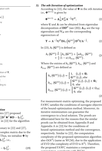
3). The nth Iteration of optimization

According to [22], the value ofin thenth iteration,

i.e.,(n+1)is given by

(n+1)₌ 12

MVHM−

1

2_UH_{, (22)}

whereUandcan be obtained from eigenvalue

decomposition ofDDH(see (20)); Mare the top

eigenvalues andVMare the corresponding

eigenvectors of

For measurement-matrix optimizing, the proposed FAWC satisfies the conditions of surrogate objective of the bound-optimization method. Moreover, its iterative minimization can guarantee the

convergence to a local solution. The proofs are abbreviated here for the reasons that the similar proofs can be obtained from Appendix B and Appendix A in [22] for the conditions of

bound-optimization method and the convergence, respectively. Similar to [22], the computation complexity of the proposed optimization algorithm is

alsoO(N3)(same as WCM), due to the application

of EVD (the complexity of EVD isN3). Therefore,

the proposed FAWC maintains a comparative computation-complexity with WCM.

4 CFO estimation method

4.1 Sparse reconstruction of EMV

In this subsection, we will present the proposed MFB-CoSaMP reconstruction-method for EMV (i.e., recov-ery. The proposed reconstruction-method mainly exploits EMV features as priori information, and thus improves its reconstruction-accuracy. We denote the reconstructed

EMV asand implement the CFO estimations (includ-ing coarse and fine CFO estimation) on the basis of the reconstructed EMV.

Among these currently available CS signal recovery algorithms, our proposed MFB-CoSaMP mainly refer-ences the CoSaMP algorithm due to its high reconstruc-tion accuracy and excellent robustness to noise [23, 24]. By further referencing the methodology of model-based CoSaMP [28], an excellent method of support-set identi-fication is developed. The objective of MFB-CoSaMP is

to recovery the EMV, i.e., the algorithm output is. We describe some critical points of MFB-CoSaMP in detail as follows.

A.1 Initialization of MFB-CoSaMP

The input parameters and initialization of MFB-CoSaMP are similar to the MFB-CoSaMP algorithm. As for the input parameters, we also need the measurement matrix , the noisy measurementsyand the sparsity levelK. In the initialization step, the initial target vector(

0)

and ini-tial residualvare, respectively, set as a zero vector andy, for the reason that no priori can be obtained.

A.2 Identification based on EMV proxy

Similar to classical CoSaMP algorithm in [23, 24], we form an EMV proxyufor CFO estimation, i.e,

u=Hv, (26)

where is the measurement matrix optimized in Section 3, and v is the residual of each iteration. For description convenience, theP×1 vectoruis expressed as u =[u1,u2, ...,uP]T. Unlike CoSaMP algorithm in which 2K largest components of the proxy u are located, the MFB-CoSaMP firstly locates the maximal amplitude inu, i.e.,

W1= {i:|ui| =max{|u1|,|u2|,· · ·,|uP|}}. (27)

According to theW1, we then locate the other 2K−1 indexes to form support-set W1. In CoSaMP, the signal components that carry a lot of energy locate in the iden-tification process whereas the EMV features indicate that the significant amplitudes only gather in one circle cluster. Thus, the maximal amplitude is of the special impor-tance to determine the location of circle cluster due to its usual high reliability. Starting from W1, we then search 2K−1 indexes nearestW1to form a circle cluster. The

identification-result, i.e., the support setW1, is given by

W1=W11 W12, (28)

whereW11is defined as

W11=

⎧ ⎪ ⎪ ⎨ ⎪ ⎪ ⎩

fI(W1−K)

,

ifufI(W1−K)≥ufI(W1+K);

fI(W1+K)

,

ifufI(W1−K)<ufI(W1+K).

(29)

WherefI(X)is an index-indication function defined as

fI(X)=

⎧ ⎨ ⎩

P+X, if X≤0 X, if 0<X≤P X−P, other

. (30)

In (28),W12is determined by the different values ofW1:

W12=

⎧ ⎪ ⎪ ⎪ ⎪ ⎨ ⎪ ⎪ ⎪ ⎪ ⎩

1,· · ·,fI(W1+K−1)

!

{W1−K+1,· · ·,P},W1>P−K+1; {1,_! · · ·,W1+K−1}

fI(W1−K+1),· · ·,P

,W1<K; {W1−K+1,· · ·,W1+K−1}, other.

(31)

A.3 Support-set merger and metric-vector estimation After obtaining the identified support-setW1, we unite

the support-set of current approximation( k−1)

to con-struct a merger support-set T in thekth iteration, i.e.,

T←supp

"

(k−1)# W1. (32)

Based on the merged support-set T, a least-square esti-mation is employed. Denotingbasb=[b1,b2, ...,bP]Tand the estimated metric-vector asb|T, we have

b|T ←(T)†y. (33)

Besides the estimated componentsb|T, the other com-ponents ofbare set as zeros, i.e.,

b|Tc ←0. (34)

Compared with CoSaMP algorithm, the procedures of support-set merger and metric-vector estimation in the proposed MFB-CoSaMP are similar, just with different support-set T.

A.4 Identification based on EMV

In CoSaMP algorithm, K largest components of the estimatedb are located. By contrast, the MFB-CoSaMP locates the maximal amplitude inb, i.e.,

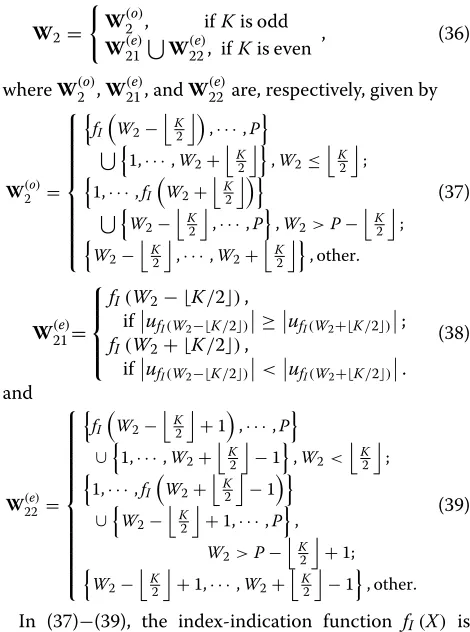
W2= {i:|bi| =max{|b1|,|b2|,· · ·,|bP|}}. (35)

identification-result, i.e., the support setW2, is given by defined in Eq. (30).

With the novel support-setW2, the components ofb which indexes lie inW2are reserved, while the others are set as zeros, i.e.,

bWc₂ ←0. (40)

A.5) Update of EMV

In the kth iteration, the metric vector( k)

should be updated according tobin (33), (34), and (40). Then, we have

(k)←b. (41)

With current samplesyand updated metric-vector(k), the residualv(i.e., the part of the metric-vector that has not been approximated) is replaced by

v←y−( k)

. (42)

AfterKiterations fromA.2toA.5, the halting criterion of MFB-CoSaMP is satisfied. Therefore, the reconstructed

A summary of MFB-CoSaMP algorithm is exhibited in Table 2. Compared with the classic CoSaMP, the proposed

Table 2MFB-CoSaMP algorithm

Input:Measurement matrix, noisy measurementsy, and sparsity levelK. Output:CFO EMV c). Identify the circle-cluster location according tou

W1= {i:|ui| =max{|u1|,|u2|,· · ·,|uP|}};

W1←the 2K indexes nearest toW1in index set{1, 2,· · ·,P}includingW1.

d). Merge the support set:

T_←supp

g). Identify circle-cluster location according tob W2= {i:|bi| =max{|b1|,|b2|,· · ·,|bP|}};

W2←theKindexes nearest toW2in index set{1, 2,· · ·,P}includingW2.

h).b_Wc 2 ←0.

i). Prune to obtain the next approximation:

MFB-CoSaMP can improve the reconstruction accuracy due to its priori information exploited from the EMV fea-tures. In CoSaMP algorithm, the support setW1locates 2Klargest components of{|u1|,|u2|, ...,|uP|}. Based on the EMV features that the significant amplitudes gather in a circle cluster, the MFB-CoSaMP first locates the index of maximal amplitude inuin theW1identification and then search the 2K−1 indexes nearest to it. The method ofW1 identification is also adopted forW2identification, except for theKlargest components of{|b1|,|b2|, ...,|bP|}with the support setW2. In MFB-CoSaMP, the maximum of ampli-tudes is of special importance to determine the location of circle cluster due to its usual highest reliability.

the totalP×1 space. Thus, the classic CoSaMP requires

2K

i=1(P−i) +

K

i=1(P−i) real additions in each iter-ation. In comparison to CoSaMP, MFB-CoSaMP only locates the maximum ofu(orb) in the totalP×1 space inA.2(orA.4), and directly chooses the locations of the other 2K −1 (or K −1 ) components whose locations are located nearest to the location of the maximum. Then, MFB-CoSaMP requires 2Preal additions in each iteration. Obviously, 2P < 2_i=1K (P−i) + K_i=1(P−i) for rea-sonable K ≥ 1. Therefore, the proposed MFB-CoSaMP reduces the computational complexity compared to the classic CoSaMP.

4.2 Coarse CFO estimation

Represented by the coarse CFO estimation, denoted as %fcoarse, the reconstructed EMV, i.e.,

4.3 Fine CFO estimation

To implement the fine CFO estimation, we first utilize the reconstructed EMV to recover the received signalrwith Nyquist rate. Then, an interpolation method is employed to construct the equivalent likelihood-function. Finally, we seek the local maximum by using the constructed likelihood-function to estimate the fine CFO.

From (9), we have r = †. With the reconstructed EMV (i.e.,), the received signalr(sampled with Nyquist rate) can be expressed as

r=†

"

+n

#

=†+†n, (45)

wherenis theN×1 noise vector, which is caused by the inaccurate reconstruction and approximate sparsity of. Then, an approximation ofr, denoted asr, can be given by

r =†=r−†n. (46)

In (46), if the dominant element-amplitudes in EMV (i.e.,

) can be reconstructed accurately and its well sparse-representation can be obtained, the effect of the noise vector n will be insignificant. Fortunately, with a good recovery-algorithm (e.g., MFB-CoSaMP) and sufficient observations (i.e., relatively large N) at a relatively high CNR, it is feasible to ignore the effect of noise vectorn.

With the recovered r and the coarse CFO estimation %fcoarse, we estimate the fine CFO (denoted as%ffine) near to%fcoarse, where the frequency range for searching%ffine is assumed to be %fcoarse−ζ,%fcoarse+ζ

withζ > 0. Without loss of generality,ζ is chosen as the half search-step of the coarse CFO estimation.

According to Eq. (6), we use the tentative frequencyf in %fcoarse−ζ,%fcoarse+ζ

to constructN ×1 vector

(in (47)), respectively, we express the equivalent

likelihood function as

Thus, the fine CFO estimation %ffinecan be obtained by seeking the maximum of the equivalent likelihood

function

In (49), the pseudo-inverse † can be computed and stored in advance to save the processing resources during the fine CFO estimation.

5 Performance evaluation

In this section, we will evaluate the performance of pro-posed methods. For the propro-posed FAWC, we will evaluate its cost function, recovery performance, and robustness. To evaluate the proposed MFB-CoSaMP, we will con-sider the reconstruction accuracy and robustness. For their combines, the coarse and fine CFO-estimations are evaluated, respectively.

5.1 Performance of optimized measurement-matrix

To verify the effectiveness of the proposed optimization-method FAWC in Section 3, comparisons against the WCM method in [22] are given in this subsection.

0 20 40 60 80 100 0

50 100 150 200 250 300

Iteration number

Value of cost function

WCM (α=0.1)

WCM (α=0.9)

WCM (α=0.99)

Proposed FAWC(α=0.1) Proposed

FAWC(α=0.9)

Proposed FAWC(α=0.99)

Fig. 3The cost functions of different construction methods, i.e., the proposed FAWC method and WCM method, whereN=128, P=128,K=5, andM=64. Three cases, i.e.,α=0.1,α=0.9, and α=0.99 are considered

α = 0.9, andα = 0.99 are, respectively, considered. For both FAWC and WCM with a relatively large number of iterations, the increasing α decreases the value of cost function of FAWC. After around 20 iterations, the pro-posed FAWC has a stable value of cost function, while jumping occurs in WCM. Furthermore, for the given dic-tionaryD = †according to the tentative CFOs, FAWC has a smaller value of cost function to capture small coher-ence of concerned patterns and non-concerned patterns.

Similar to the WCM,α ≈ 1 is also a good value for the proposed FAWC method. To avoid completely ignoring the coherence of non-concerned patterns, settingα = 1 is not considered in the following simulations of this sub-section. At the same time, for the sake of fairness, both WCM and proposed FAWC method employ the classic CoSaMP method to reconstruct EMV. Note that we do not adopt the proposed MFB-CoSaMP for the EMV recov-ery in this subsection. We just expect to actually reveal the improvement from the optimization of measurement matrix, rather than our reconstruction method. We will evaluate the MSE performance, and the MSE in this paper is defined as

MSE=E$X−%X 2 2 X2₂

(

, (50)

where E{·} denotes the expectation operator, %X is the estimation ofX.

The MSE performance of EMV recovery is given in Figs. 4 and 5, where N = 128, P = N = 128, α = 0.9, and the reconstruction method is classic CoSaMP. Note that the main purpose of introducing the circle-cluster in Section 3 is to solve the uncertainty of sub-block when the

8 12 16 20 24 28 10−1

100

CNR(dB)

MSE

Proposed FAWC (K=7) WCM (K=7) Proposed FAWC (K=9) WCM (K=9) Proposed FAWC (K=13) WMC (K=13)

Fig. 4MSE vs. CNR with different measurement-matrices (optimized by WCM and proposed FAWC, respectively) and sparsityK, where N=128,P=128,α=0.9, andM=64 are considered

normalized CFO is near to+0.5 or−0.5. For other cases with the same CoSaMP recovery algorithm, similar MSE performance can be obtained from the two optimization methods. Thus, in this simulation, the unknown normal-ized CFO randomly generated is near to+0.5 or−0.5. We employ the interval [ 0.45, 0.5)!(−0.5,−0.45] to repre-sent the space near to+0.5 or−0.5. TheK-sparsity EMV is formed in each simulation by the following procedure: (a) generate a noise-free EMV with a normalized-CFO near to +0.5 or −0.5 randomly; (b) find the maximum among EMV element-amplitudes; (c) set the elements in EMV to zeros except the maximum-amplitude element and the other K − 1 elements which indexes are the

8 12 16 20 24 28 10−1

100

CNR(dB)

MSE

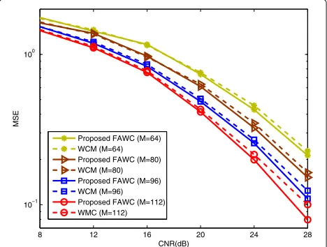
Proposed FAWC (M=64) WCM (M=64) Proposed FAWC (M=80) WCM (M=80) Proposed FAWC (M=96) WCM (M=96) Proposed FAWC (M=112) WMC (M=112)

nearest to the maximum-amplitude element (similar to form theW2inA.4of Section 4). The formed EMV passes through the noise channel and then generates measure-ments according to the different measurement matrices optimize by WCM and proposed optimization-method, respectively. DifferentKs are adopted whileMis kept as N/2 = 64 unchanged in Fig. 4. From Fig. 4, the pro-posed FAWC optimization-method slightly reduces the MSE, compared with WCM. With the increasing K, a much easier distinguishment of MSE improvement can be observed, due to the increasing significance of suitable concerned-patterns with a largerK. The similar conclu-sions can also be seen in Fig. 5, where different M are adopted whileK is kept as 13. From Fig. 5, the proposed FAWC optimization-method slightly improves the MSE performance.

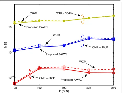
In Fig. 6,M,P, andKvary according to the varyingNis simulated, whereM=N/2,P=N,K= N/10,α=0.9, and three cases of CNR (i.e., ρ = 30 dB,ρ = 40 dB, and ρ = 50 dB) are considered. From Fig. 6, with the increasing CNR, the improvement of MSE is observed apparently.

Besides coping with the uncertainty of sub-block, the proposed optimization-method can also help to improve the proposed reconstruction method, which can be seen in the later simulations.

5.2 Effectiveness of MFB-CoSaMP

In this subsection, we compare the reconstruction per-formance of EMV when CoSaMP and MFB-CoSaMP are, respectively, adopted. To really present the merits of MFB-CoSaMP, a Gaussian random matrix [16], which is generated with each entry independently drawn from a Gaussian distribution with zero mean and unit vari-ance, is employed as the measurement matrix for both

128 160 192 224 256 10−3

10−2 10−1

P (or N)

MSE

WCM

WCM CNR = 30dB

CNR = 40dB

WCM

CNR = 50dB Proposed FAWC

Proposed FAWC

Proposed FAWC

Fig. 6MSE vs.P(orN) with different measurement-matrices (optimized by WCM and FAWC respectively), whereM=N/2,P=N, α=0.9, andK= N/10are, respectively, considered

algorithms. We do not use the optimized measurement matrices (e.g., the matrix optimized by WCM method or proposed FAWC in this paper) to avoid any improvement brought from the optimization of measurement matrix.

Similar to the MSE evaluation in Subsection 5.1 of this section, the same procedure is adopted to generate K-sparsity EMV and to pass through the noise chan-nel. Then, we employ Gaussian random-matrix to com-press EMV and obtain the measurements. To compare the reconstruction performance of CoSaMP and MFB-CoSaMP, Figs. 7, 8, and 9 give the MSE performance. In Fig. 7, the MSE performance with different sparsityKs are considered (i.e.,K=7,K =9, andK=13), andN=128, P = N = 128, M = N/2 = 64. It can be seen that the proposed MFB-CoSaMP effectively reduces MSE rel-ative to the classic CoSaMP. The similar conclusion can also be derived from the cases of Figs. 8 and 9. In Fig. 8, the MSE comparison with different numbers of measure-ment, whereN = 128,P = N = 128,K = 13, and four cases of measurements (i.e.,M= 64,M = 80,M = 96, andM=112) are considered. Particularly, in Fig. 9, theM, P, andK are approximate linear-varying with the change of N, i.e., N varies from 128 to 256, while M = N/2, P = N, andK = N/20. Actually,Kdoes not vary lin-early withN, describing its as approximate linear-varying for description convenience. Besides these basic param-eters, three cases of CNR, i.e.,ρ = 10 dB,ρ = 20 dB, andρ = 30 dB are considered. Compared with CoSaMP, the MFB-CoSaMP obviously improve the MSE perfor-mance in Figs. 8 and 9. Besides the MSE improvement, Fig. 9 also illuminates that more significant improvement can be obtained with the increase of CNR, due to more remarkable EMV features in the higher CNR. The MSE

8 10 12 14 16 18 20 22 24 26 28 10−1

100

CNR(dB)

MSE

MFB−CoSaMP (K=7) CoSaMP (K=7) MFB−CoSaMP (K=9) CoSaMP (K=9) MFB−CoSaMP (K=13) CoSaMP (K=13)

Proposed MFB−CoSaMp

CoSaMP

8 10 12 14 16 18 20 22 24 26 28 10−1

100

CNR(dB)

MSE _{MFB−CoSaMP (M=64)}

CoSaMP (M=64) MFB−CoSaMP (M=80) CoSaMP (M=80) MFB−CoSaMP (M=96) CoSaMP (M=96) MFB−CoSaMP (M=112) CoSaMP (M=112)

CoSaMP

Proposed MFB−CoSaMP

Fig. 8MSE of EMV reconstruction with different reconstruction algorithms (i.e., CoSaMP and proposed MFB-CoSaMP) and differentM (i.e.,M=64,M=80,M=96, andM=112). WhereN=128, P=N=128, andK=13 are considered

performance improvements in Figs. 7, 8, and 9 are mainly due to the prior-information developed from the EMV features (see step c and g) in Table 2, or seeA.2andA.4in Subsection 4.1 for details).

5.3 Performance of CFO estimation

In this subsection, we discuss the influence of proposed methods in the coarse and fine CFO estimation, respec-tively. For the convenience of expression, some abbrevia-tions are given as follows.

• “WCM + CoSaMP” denotes that the measurement

matrix is optimized by WCM method, and the reconstruction algorithm is CoSaMP.

128 160 192 224 256 10−1

100 101

N

MSE

MFB−CoSaMP (CNR=10dB) CoSaMP (CNR=10dB) MFB−CoSaMP (CNR=20dB) CoSaMP (CNR=20dB) MFB−CoSaMP (CNR=30dB) CoSaMP (CNR=30dB)

CNR=10dB

CNR=20dB

CNR=30dB

Fig. 9MSE of EMV reconstruction with different reconstruction algorithms (i.e., CoSaMP and proposed MFB-CoSaMP) and differentN. WhereM,P, andKvary withN, i.e.,M=N/2,P=N, andK= N/20, three cases of CNR, i.e.,ρ=10 dB,ρ=20 dB, andρ=30 dB are, respectively, considered

• “FAWC + CoSaMP” represents that the

measurement matrix is optimized by proposed FAWC optimization method, and the reconstruction algorithm is CoSaMP.

• “WCM + MFB-CoSaMP” denotes that the

measurement matrix is optimized by WCM method, and the reconstruction algorithm is MFB-CoSaMP.

• “FAWC + MFB-CoSaMP” represents that the

measurement matrix is optimized by FAWC, and the reconstruction algorithm is MFB-CoSaMP.

• “ML (Nyquist Rate)” denotes ML-based coarse CFO

estimation with the Nyquist-rate sampling.

Unlike the known sparsity in aforementioned simu-lations, the sparsity K during the CFO estimation is usually unknown in practical systems. Thus, a spar-sity level (i.e., inexact sparspar-sity) is employed in this Section. To obtain a reasonable sparsity level, we use the maximum-amplitude of EMV to set the thresh-old. The maximum-amplitude can be expressed as γ =max

f1,

f2,· · ·,

fP

, where

fp˜

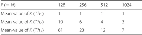
,p = 1, 2,· · ·,Pis defined in (4). Three thresh-olds, i.e.,Th1=0.1×γ,Th2=0.05×γ, andTh3=0.01×

γ, are considered. The amplitude larger than Thi,i = 1, 2, 3, is viewed as the significant amplitude under the thresholdThi, and the number of significant amplitudes is counted as sparsity-Kin each experiment. The 105 statis-tical experiment results are given in Tables 3 and 4, where the ceiling operator is employed to make the mean value and variance be an integer.

From Tables 3 and 4, choosing the moderate threshold Th2 can commendably cover significant amplitudes and holds a relatively smallKfor a good reconstruction accu-racy, whileTh3keeps a better approximation at the cost of a biggerK. In this paper, we always consider the case P=N. IncreasingPorNcan make the significant ampli-tudes of EMV more concentrated and easier to cover with a smallerK. The sparsity levels are given as follows.

• ForN=128, we chooseK=10as the sparsity-level

according to its mean withTh2. BecauseTh1is high

and only one element of EMV is reserved (according

to the mean),Th3results in a too bigK to ensure the

measurementsMN.

• ForN=256, we would like to choose the sparsity

level asK=23according to the mean withTh3.

Table 3Mean value of spasity-Kwith different thresholds

P(=N) 128 256 512 1024

Mean-value ofK(Th1) 1 1 1 1

Mean-value ofK(Th2) 10 6 4 3

Table 4Variance of spasity-Kwith different thresholds

P₍₌N₎ 128 256 512 1024

Variance ofK₍T h1) 0 0 0 0

Variance ofK(T h2) 35 36 23 13

Variance ofK(T h3) 1792 828 503 278

• ForN=512andN=1024, the thresholdTh3is

usually employed, while the mean and variance with

Th3are simultaneously considered, sinceN is large

enough to cover more significant-amplitudes of EMV. Then, the sparsity levels are, respectively, chosen as

35 (12+

,_√

503

-) and 37 (7+.√3×287/).

• For simulation convenience, we also choose

sparsity-level asK = N/10in some simulations.

C.1 Performance evaluation of coarse CFO estimation

Compared with the WCM optimization, we firstly ver-ify the correct probability of coarse CFO-estimation can be improved by using the proposed FAWC. The correct coarse CFO estimation is defined as

f −%fcoarseTs≤

2, (51)

i.e., the offset between the estimated CFO and the real CFO is no more than a half search-step. In this paper, the search-step for coarse CFO estimation is set as = 1/P.

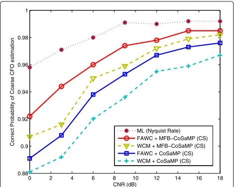
The correct probability of coarse CFO estimation is given in Fig. 10, where N = 128, P = N = 128, α = 0.9, M = N/2 = 64, and K = 10 (according to Th2 in Table 3). The measurement matrix is opti-mized by FAWC and WCM, respectively. As for the unknown normalized CFO, which is randomly generated in [ 4.5,+0.5)or(−0.5,−4.5] to illuminate the proposed optimization method, can solve the uncertainty of sub-block. Compared with “WCM + CoSaMP”, “FAWC + CoSaMP” proves that the proposed measurement matrix can improve the correct probability due to its same recovery algorithm (i.e., CoSaMP). Similar to “WCM + CoSaMP”, “WCM + MFB-CoSaMP” shows recovery effec-tiveness of MFB-CoSaMP since the WCM is utilized in both methods. Although MFB-CoSaMP presents a sig-nificant improvement relative to “WCM + CoSaMP”, the proposed measurement matrix (i.e., the measure-ment matrix optimized by the FAWC) can arouse further improvement. Thus, the correct probability of “FAWC + MFB-CoSaMP”, which is nearest to that of ML, can obtain the best improvement of coarse CFO estimation. Figure 10 manifests the effectiveness of the FAWC and MFB-CoSaMP, i.e., FAWC and MFB-CoSaMP can inde-pendently or jointly improve the correct probability of coarse CFO estimation.

0 2 4 6 8 10 12 14 16 18 0.88

0.9 0.92 0.94 0.96 0.98 1

CNR (dB)

Correct Probability of Coarse CFO estimation

ML (Nyquist Rate) FAWC + MFB−CoSaMP (CS) WCM + MFB−CoSaMP (CS) FAWC + CoSaMP (CS) WCM + CoSaMP (CS)

Fig. 10Correct probability of coarse CFO estimation. Where different measurement-matrices (i.e., constructed by the proposed FAWC method and WCM method),N₌128,P₌N₌128,_α=0.9,K₌10, andM₌N_/2₌64 are considered

To elaborate the parameter influence, we, respectively, investigate the influences ofK,M, andN in Figs. 11, 12, and 13, where normalized CFO is randomly generated in [−0.5,+0.5). With different K (i.e., K = 7,K = 9, K = 13) and the same other parameters of the simu-lation in Fig. 10, the correct probability of coarse CFO estimation is given in Fig. 11. Again, we can see that the proposed FAWC and MFB-CoSaMP can jointly improve the correct-probability of coarse CFO estimation, com-pared with “WCM + CoSaMP”. Besides the improvement

−8 −4 0 4 8 12 16 0.4

0.5 0.6 0.7 0.8 0.9 1

CNR (dB)

Correct Probability of Coarse CFO estimation

ML (Nyquist Rate) FAWC + MFB−CoSaMP(K=7) WCM + CoSaMP(K=7) FAWC+ MFB−CoSaMP(K=9) WCM + CoSaMP(K=9) FAWC + MFB−CoSaMP(K=13) WCM + CoSaMP(K=13)

−8 −4 0 4 8 12 16 0.7

0.75 0.8 0.85 0.9 0.95 1

CNR (dB)

Correct Probability of Coarse CFO estimation

ML (Nyquist Rate) FAWC + MFB−CoSaMP (M=80) WCM + CoSaMP (M=80) FAWC + MFB−CoSaMP (M=96) WCM + CoSaMP (M=96) FAWC + MFB−CoSaMP (M=112) WCM + CoSaMP (M=112)

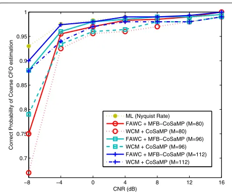
Fig. 12Correct probability of coarse CFO estimation with differentM. WhereN=128,P=N=128,α=0.9,K=13, different

measurement-matrices (i.e., constructed by FAWC method and WCM method), and differentM(i.e.,M=80,M=96, andM=112) are considered

of correct probability, it looks like the smallerK(near the sparsity-levelK = 10) obtains better correct probabil-ity when CNR is relatively low (e.g.,ρ ≤ −4 dB). When ρ ≥ −4 dB, the influence ofK(near the sparsity-level) is not clear.

During the simulation in Fig. 11, we fix sparsityK=13 (near to 10, andN/10 = 128/10=13), changeM, and keep other parameters the same. The curves of correct probability with differentMare plotted in Fig. 12, where

−8 −6 −4 −2 0 2 4 6 8 0.65

0.7 0.75 0.8 0.85 0.9 0.95 1

CNR (dB)

Correct Probability of Coarse CFO estimation

FAWC + MFB−CoSaMP (N=160) WCM + CoSaMP (N=160) FAWC + MFB−CoSaMP (N=192) WCM + CoSaMP (N=192) FAWC + MFB−CoSaMP (N=224) WCM + CoSaMP (N=224) FAWC + MFB−CoSaMP (N=256) WCM + CoSaMP (N=256)

Fig. 13Correct probability of coarse CFO estimation with differentN. WhereP=N,M=N/2α=0.9,K=13, different measurement-matrices (i.e., constructed by FAWC method and WCM method), and different N(i.e.,N=160,N=192,N=224 andN=256) are considered

N = 128, P = N = 128, α = 0.9, K = 13, differ-ent measuremdiffer-ent-matrices (i.e., optimized by the FAWC method and WCM method), and differentMs (i.e.,M= 80, M = 96, and M = 112) are considered.With the increase ofM, higher correct probability can be obtained, and the improvement is much easier to observe in lower CNR. In Fig. 13, M, P, and K vary with the change of N, whereM = N/2, P = N, α = 0.9, K = N/10. Compared with “WCM + CoSaMP”, the “FAWC + MFB-CoSaMP” improve the correct probability of coarse CFO estimation. When CNR is relatively low, e.g.,ρ ≤ −4 dB, the biggerNobtains a higher correct probability for both “WCM + CoSaMP” and “FAWC + MFB-CoSaMP”, while this rule is not certain for higher CNR. Even so, it is clear that the improvement from “FAWC + MFB-CoSaMP” obviously exists.

According to the aforementioned coarse CFO esti-mation, our “FAWC + MFB-CoSaMP” can effectively improve its correct probability compared with the con-ventional “WCM + CoSaMP”.

C.2 Performance of fine CFO estimation

Under the compressive sampling scenario, our objec-tive is to obtain a better MSE of fine CFO-estimation, compared with the conventional CS-based method. Fur-thermore, the MSE performance, which can reach the Crame´r-Rao lower Bound (CRLB) of Nyquist rate, is also expected. From [15], the CRLB with Nyquist rate is given by

CRLB= 3 2π2_T2

s

· 1

ρNN2₋₁. (52)

where the CNRρis defined in (2).

Firstly, we investigate the MSE performance of fine CFO estimation with different numbers of measurement. The performance evaluation is given in Fig. 14, whereN=128 P=N,α=0.9,K =10, different measurement matrices (i.e., constructed by the proposed optimization method and WCM method), and differentM(i.e.,M = 64,M= 96, andM = 112) are considered. From Fig. 14, the pro-posed method, i.e., “FAWC + MFB-CoSaMP”, improves the MSE performance, compared with the conventional “WCM + CoSaMP”. It is obvious that the increasingM makes a better MSE for both “FAWC + MFB-CoSaMP” and “WCM + CoSaMP”. Regrettably, sustained increasing ofMcannot obtain significant MSE-improvement for the relative large M (e.g.,M ≥ 96) and relative high CNR (CNRρ≥ −2 dB).

−8 −6 −4 −2 0 2 4 6 8 10−8

10−7 10−6 10−5 10−4 10−3 10−2 10−1

CNR(dB)

MSE

WCM+CoSaMP(M=64) FAWC+MFB−CoSaMP(M=64) WCM+CoSaMP(M=96) FAWC+MFB−CoSaMP(M=96) WCM+CoSaMP(M=112) FAWC+MFB−CoSaMP(M=112) ML (Nyquist Rate) CRLB(Nyquist Rate)

Fig. 14MSE of fine CFO-estimation with differentM. WhereN=128 P=N,α=0.9,K=10 (according to Table 3), different

measurement-matrices (i.e., constructed by the proposed FAWC method and WCM method), and differentM(i.e.,M=64,M=96, andM=112) are considered

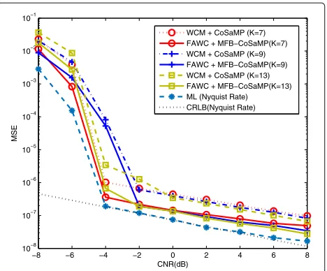
i.e., “FAWC + MFB-CoSaMP”, has a better MSE perfor-mance than conventional “WCM + CoSaMP”. For both “FAWC + MFB-CoSaMP” and “WCM + CoSaMP”, the smallest MSE is reached at K = 7 under the low CNR (e.g.,ρ≤ −2 dB). When CNR is high (e.g.,ρ≥2 dB) the smallest MSE is obtained byK = 13. That is to say, the higher CNR or the lower noise makes a largerKwhich is chosen to cover enough significant amplitudes and get a

−8 −6 −4 −2 0 2 4 6 8 10−8

10−7 10−6 10−5 10−4 10−3 10−2 10−1

CNR(dB)

MSE

WCM + CoSaMP (K=7) FAWC + MFB−CoSaMP(K=7) WCM + CoSaMP (K=9) FAWC + MFB−CoSaMP(K=9) WCM + CoSaMP (K=13) FAWC + MFB−CoSaMP(K=13) ML (Nyquist Rate) CRLB(Nyquist Rate)

Fig. 15MSE of fine CFO-estimation with differentK. WhereN=128 P=N,M=96,α=0.9, different measurement-matrices (i.e., constructed by the FAWC method and WCM method), and differentK (i.e.,K=7,K=9, andK=13) are considered

better EMV approximation. Actually, the influence of the given sparsity-Kin Fig. 15 is not significant.

Unlike coarse CFO-estimation that only EMV requires to recover, the fine CFO-estimation usually need the recovered signalrat Nyquist rate to construct the equiv-alent likelihood function (see Subsection 4.1). An approx-imation of received signal ris given in (46). In (46), we require a good enough approximation of EMV, and thus the enough “energy” of EMV could be covered. It looks like a largerK is more effective for a relative high CNR (e.g., in Fig. 15). However, larger K usually results in a worse reconstruction accuracy. From Tables 3 and 4, a larger N can make the “energy” more concentrated in EMV. To balanceKand covered “energy”, a largerNis a good choice.

To verify the feasibility that the largerNcan get the bet-ter MSE performance, the simulation is given in Fig. 16, whereP=N,M= 0.85×N,K = 0.1×N,α =0.9, N = 128, N = 192, and N = 256 are, respectively, considered. As we expected, increasingNcan reduce the MSE for both “FAWC + MFB-CoSaMP” and “WCM + CoSaMP”, and the proposed “FAWC + MFB-CoSaMP” can obtain a smaller MSE than “WCM + CoSaMP” for eachN. Another phenomenon observed in Fig. 16 is that the largerN, the closer MSE to its CRLB could be obtained. To verify this, an extended simulation is given in Fig. 17, where P = N, M = 0.85 × N, K = 0.1 × N, α = 0.9, and three cases ofN (i.e.,N = 256,N = 512, andN=1024) are considered. It is obvious that the large N can make MSE easily reach the CRLB in spite of the insignificant discrepancy.

−12 −8 −4 0 4 8 12 10−9

10−8 10−7 10−6 10−5 10−4 10−3 10−2 10−1

CNR(dB)

MSE

WCM + CoSaMP (N=128) FAWC + MFB−CoSaMP(N=128) WCM + CoSaMP (N=192) FAWC + MFB−CoSaMP(N=192) WCM + CoSaMP (N=256) FAWC + MFB−CoSaMP(N=256) ML (Nyquist Rate, N=128) CRLB (Nyquist Rate, N=128) ML (Nyquist Rate, N=192) CRLB (Nyquist Rate, N=192) ML (Nyquist Rate, N=256) CRLB (Nyquist Rate, N=256)

−8 −6 −4 −2 0 2 4 6 8 10 12 10−11

10−10 10−9 10−8 10−7 10−6 10−5 10−4 10−3

CNR(dB)

MSE

WCM + CoSaMP (N=256) FAWC + MFB−CoSaMP(N=256) CRLB(Nyquist Rate, N=256) WCM + CoSaMP (N=512) FAWC + MFB−CoSaMP(N=512) CRLB(Nyquist Rate, N=512) WCM + CoSaMP (N=1024) FAWC + MFB−CoSaMP(N=1024) CRLB(Nyquist Rate, N=1024)

N=256

N=1024 N=512

Fig. 17MSE of fine CFO-estimation with differentN. WhereP=N, M= 0.85×N,K= 0.1×N,α=0.9, different measurement-matrices (i.e., constructed by the proposed FAWC method and WCM method), and differentNi.e.,N=256,N=512, andN=1024, are considered

6 Conclusions

In this paper, a preliminary study for CFO estimation based on compressed sensing has been exhibited. We first confirmed that compressive sampling is feasible for ML-based CFO estimation. To solve the number uncertainty of sub-block in block-sparsity CS scenarios, we then intro-duce the circle cluster, propose a new coherence-pattern, and form an FAWC optimization-method by exploiting the features of EMV. Compared with WMC, the proposed FAWC shows improvements in full-performance evalua-tions. FAWC can obtain smaller value of cost function to capture small coherence, can obtain a better convergence. Beside the properties of small coherence and good con-vergence, FAWC effectively solves the uncertainty of sub-block and thus improve the reconstruction accuracy and robustness to sparsity level, receive signal length, and the measurements. Furthermore, based on the EMV features, the MFB-CoSaMP is proposed to boost the support set mergence, improve the reconstruction accuracy, reduce the computational complexity, and hold the improvement robustness against the simulation parameters. Finally, the jointed “FAWC + MFB-CoSaMP” has been verified by the elaborate performance evaluations. For example, the MSE performance which is close to the CRLB is better than that of “WCM + CoSaMP”, “WCM + MFB-CoSaMP”, or “FAWC + MFB-CoSaMP”, while the improvement is robust to the simulation parameters (e.g., sparsity level, number of measurement, and receive signal length).

Acknowledgements

The authors wish to thank the editor and the anonymous reviewers for their valuable suggestions, which helped significantly improve the quality of the paper. This work is supported in part by the project of Meteorological information and Signal Processing Key Laboratory of Sichuan Higher Education Institutes (Grant No. QXXCSYS201402), the project of science and

technology plan of Sichuan Province (Grant No. 2015JY0138), the Xihua University Young Scholars Training Program (Grant No. 01201408 ), the key scientific research fund of Xihua University (Grant No: Z1120941, Z1120945, Z1320927), the key projects of Education Department of Sichuan Province (Grant No. 15ZA0134), the Open Research Subject of Key Laboratory (Research Base) of signal and information processing (Grant No. szjj2015-071), and the Chunhui plan of Ministry of education (Grant No. Z2015113) of China.

Authors’ contributions

All authors read and approved the final manuscript.

Competing interests

The authors declare that they have no competing interests.

Author details

1_{School of Electrical Engineering and Electronic Information, Xihua University,}

610039 Chengdu, China.2_{Department of Electrical and Computer} Engineering, Texas A&M University, College Station, 77840 Texas, USA. 3_{National Key Laboratory of Science and Technology on Communications,}

University of Electronic Science and Technology of China, 611731 Chengdu, China.4_{Alps Electric Co., Ltd., 141–8501 Tokyo, Japan.}

Received: 10 April 2016 Accepted: 15 September 2016

References

1. L Haring, A Czylwik, M Speth, inProc. 2004 International OFDM-Workshop. Analysis of synchronization impairments in multiuser OFDM systems, (Dresden, 2004), pp. 91–95

2. X Wang, B Hu, A low-complexity ML estimator for carrier and sampling frequency offsets in OFDM systems. IEEE Commun. Lett.18(3), 503–506 (2014)

3. M Morelli, U Mengali, Feedforward frequency estimation for PSK: A tutorial review. Eur. Trans. Telecommun.9(2), 103–116 (1998) 4. W Kuo, M Fitz, Frequency offset compensation of pilot symbol assisted

modulation in frequency flat fading. IEEE Trans. Commun.45(11), 1412–1416 (1997)

5. M Morelli, U Mengali, Carrier-frequency estimation for transmissions over selective channels. IEEE Trans. Commun.48(9), 1580–1589 (2000) 6. D Donoho, Compressed sensing. IEEE Trans. Inf. Theory.52(4), 1289–1306

(2006)

7. E Cands, J Romberg, T Tao, Robust uncertainty principles: exact signal reconstruction from highly incomplete frequency information. IEEE Trans. Inf. Theory.52(2), 489–509 (2006)

8. P Cheng, Z Chen, Y Guo, L Gui, inProc IEEE International Symposium on Personal Indoor and Mobile Radio Communications (PIMRC). Distributed Bayesian compressive sensing based blind carrier-frequency offset estimation for interleaved OFDMA uplink, (London, 2013), pp. 801–806 9. J Zhang, K Niu, Z He, inProc IEEE International Conference on

Communications (ICC). Multi-layer distributed Bayesian compressive sensing based blind carrier-frequency offset estimation in uplink OFDMA systems, (Kuala Lumpur, 2016), pp. 1–5

10. J Zhou, M Ramirez, S Palermo, S Hoyos, Digital-assisted asynchronous compressive sensing front-end. IEEE J. Emer. Sel. Topics Circuits Syst.2(3), 482–492 (2012)

11. X Chen, E Sobhy, Z Yu, S Hoyos, J Silva-Martinez, S Palermo, B Sadler, A sub-Nyquist rate compressive sensing data acquisition front-end. IEEE J. Emerg. Sel. Topics Circuits Syst.2(3), 542–551 (2012)

12. S Kong, A deterministic compressed GNSS acquisition technique. IEEE Trans. Veh. Technol.62(2), 511–521 (2013)

13. S Kong, B Kim, Two-dimensional compressed correlator for fast PN code acquisition. IEEE Trans. Wireless Commun.12(11), 5859–5867 (2013) 14. B Kim, S Kong, Two-dimensional compressed correlator for fast acquisition

of BOC(m, n) signals. IEEE Trans. Veh. Technol.63(6), 2662–2672 (2014) 15. M Luise, R Reggiannini, Carrier frequency recovery in all-digital modems

for burst-mode transmissions. IEEE Trans. Commun.43(234), 1169–1178 (1995)