STABILITY PROPERTIES OF STOCHASTIC VOLTERRA
INTEGRO-DIFFERENTIAL EQUATIONS
LEONID E. SHAIKHET AND JASON A. ROBERTS
Received 2 August 2004; Revised 16 January 2005; Accepted 10 April 2005
We consider the reliability of some numerical methods in preserving the stability proper-ties of the linear stochastic functional differential equationdx(t)=(αx(t) +β0tx(s)ds)dt +σx(t−τ)dW(t), whereα,β,σ,τ≥0 are real constants, andW(t) is a standard Wiener process. The areas of the regions of asymptotic stability for the class of methods consid-ered, indicated by the sufficient conditions for the discrete system, are shown to be equal in size to each other and we show that an upper bound can be put on the time-step pa-rameter for the numerical method for which the system is asymptotically mean-square stable. We illustrate our results by means of numerical experiments and various stability diagrams. We examine the extent to which the continuous system can tolerate stochastic perturbations before losing its stability properties and we illustrate how one may accu-rately choose a numerical method to preserve the stability properties of the original prob-lem in the numerical solution. Our numerical experiments also indicate that the quality of the sufficient conditions is very high.
Copyright © 2006 L. E. Shaikhet and J. A. Roberts. This is an open access article distrib-uted under the Creative Commons Attribution License, which permits unrestricted use, distribution, and reproduction in any medium, provided the original work is properly cited.
1. Introduction
Volterra integro-differential equations arise in the modelling of hereditary systems (i.e., systems where the past influences the present) such as population growth, pollution, fi-nancial markets and mechanical systems (see, e.g., [1,4]). The long-term behaviour and stability of such systems is an important area for investigation. For example—will a pop-ulation decline to dangerously low levels? Could a small change in the environmental conditions have drastic consequences on the long-term survival of the population? There is a growing body of works devoted to such investigations (see, e.g., [8,25]). Analyt-ical solutions to such problems are generally unavailable and numerAnalyt-ical methods are adopted for obtaining approximate solutions. A large number of the numerical meth-ods are developed from existing numerical methmeth-ods for systems of ordinary differential
equations (see [24] for a discussion of some of these methods for ODEs). A natural ques-tion to ask is “do the numerical soluques-tions preserve the stability properties of the exact solution?”. We refer the reader to a number of works where the answers to such questions are investigated: [2,3,6,7,9,28].
Many real-world phenomena are subject to random noise or perturbations (e.g., freak weather conditions may adversely affect the supports of a bridge, possibly changing the long-term integrity of the structure). It is a natural extension of the deterministic work carried out by ourselves and others to consider the stability of stochastic systems and of numerical solutions to such systems. We refer the readers to a number of texts which discuss the role of stochastic systems in mathematical modelling: [1,15,27]. In particular, stochastic integro-differential equations and its difference analogues are considered in [5,11–14,26].
In this paper we consider the scalar linear test equation
dx(t)=
αx(t) +β t
0x(s)ds
dt+σx(t−τ)dW(t), (1.1)
x(s)=ϕ0(s), s∈[−τ, 0], (1.2)
whereα,β,σ,τ≥0 are real constants, andW(t) is a standard Wiener process. General theory of stochastic differential equations type of (1.1) was studied by Gikhman and Sko-rokhod [10].
The selected test equation (1.1) arises from the deterministic linear test equation of Brunner and Lambert [2] ˙x(t)=αx(t) +β0tx(s)dsby replacing the parameterαwith its mean-value plus a stochastic perturbations type of the white noiseα+σW˙(t). This leads to the stochastic differential equationdx(t)=(αx(t) +β0tx(s)ds)dt+σx(t)dW(t). An addition of delayτ≥0 in the stochastic term of this equation is a quite natural generaliza-tion and leads to (1.1). The delayτdoes not have any influence on the obtained stability conditions but allows to demonstrate the construction of these conditions more com-pletely. On the other hand even forτ=0 the difference analogue of (1.1) is a difference equation with delay. So, an addition of delayτdoes not lead to the essential complication of the text.
The main conclusion of our investigation here can be formulated in the following way: if the trivial solution of the initial functional differential equation is asymptotically mean square stable then there exists a method and a step of discretization of this equa-tion so that the trivial soluequa-tion of the corresponding difference equation is asymptotically mean square stable too. Moreover, it is possible to find an upper bound for the step of discretization for which the corresponding discrete analogue preserves the properties of stability.
The conditions for asymptotic mean square stability are obtained here by virtue of Kolmanovskii and Shaikhet’s general method of Lyapunov functionals construction ([17–
23,29,31–33]) which is applicable for both differential and difference equations, both for deterministic and stochastic systems with delay.
Let us remind ourselves of some definitions and statements which will be used. Let{Ω,Ᏺ,P}be a basic probability space with a family ofσ-algebras ft⊂Ᏺ,t≥0, and Hbe a space of f0-adapted functionsϕ(s),s≤0. LetEbe the sign for expectation.
Consider a stochastic differential equation with aftereffect dx(t)=at,xt
dt+bt,xt
dW(t), x0=ϕ0∈H. (1.3)
HenceW(t)∈Rmis anm-dimensional Wiener process, the functionalsa(t,ϕ)∈Rnand b(t,ϕ)∈Rn×mare defined fort≥0,ϕ∈H,a(t, 0)=0,b(t, 0)=0.x
t(s)=x(t+s),s≤0, is a trajectory of the processx(s) fors≤t.
Definition 1.1. The trivial solution of (1.3) is called
(i) mean square stable if for every>0 there exists aδ=δ()>0 such thatE|x(t)|2< for allt≥0 if sups≤0E|ϕ(s)|2< δ;
(ii) asymptotically mean square stable if it is mean square stable and limt→∞E|x(t)|2= 0 for every initial functionϕ∈H.
LetDbe a space of functionalsV(t,ϕ), wheret≥0,ϕ∈H, for which the function Vϕ(t,x)=V
t,xt
=Vt,x,xt(s), s <0
, x=x(t), ϕ=xt, (1.4) has one continuous derivative with respect totand two continuous derivatives with re-spect tox. For each functionalV fromDthe generatorLis defined by the formula
LV(t,ϕ)= ∂
∂tVϕ(t,x) +a(t,ϕ) ∂
∂xVϕ(t,x) + 1 2tr
b(t,ϕ) ∂ 2
∂x2Vϕ(t,x)b(t,ϕ) , (1.5) where the prime symboldenotes transpose.
Theorem1.2 ([16,17]). Let there exist a functionalV=V(t,ϕ)∈Dsuch that EV(t,xt)≥c1E|x(t)|2,
EV(0,ϕ0)≤c2sup s≤0
Eϕ0(s)2,
ELV(t,xt)≤ −c3E|x(t)|2,
(1.6)
Let{Ω,Ᏺ,P}be a basic probability space, fi∈Ᏺ,i∈Z= {0, 1,...}be a sequence of σ-algebras,ξi∈Rm,i∈Zbe fi+1-adapted and mutually independent random variables. Suppose also thatEξi=0,Eξiξi=I, whereIis an identity matrix.
Consider a stochastic difference equation
xi+1=a
i,x−m,...,xi
+bi,x−m,...,xi
ξi, i∈Z. (1.7)
Herea∈Rn,b∈Rn×m,a(i, 0,..., 0)=0,b(i, 0,..., 0)=0,x
i=ϕi,i∈[−m, 0]. Definition 1.3. The trivial solution of (1.7) is called:
(i) mean square stable if for every>0 there existsδ=δ()>0 such thatE|xi|2<, i∈Z, if supi∈[−m,0]E|ϕi|2< δ;
(ii) asymptotically mean square stable if limi→∞E|xi|2=0 for every initial functionϕi. Theorem1.4 [20]. Let there exist a nonnegative functionalVi=V(i,x−m,...,xi), which satisfies the conditions
EV0,x−m,...,x0
≤c1sup i≤0
Eϕi2,
EΔVi≤ −c2Exi2, i∈Z,
(1.8)
wherec1>0,c2>0,ΔVi=Vi+1−Vi. Then the trivial solution of (1.7) is asymptotically mean square stable.
2. A linear stochastic Volterra integro-differential equation Consider (1.1). It is well known [16] that forβ=0 the inequality
2α+σ2<0 (2.1)
is the necessary and sufficient condition for the asymptotic mean square stability of the trivial solution of (1.1).
Ifσ=0 then (1.1) reduces to the Brunner and Lambert test equation [2] and also takes the differential form
¨
x(t)=αx˙(t) +βx(t). (2.2)
In this case the inequalities
α <0, β <0, (2.3)
are the necessary and sufficient condition for asymptotic stability of the trivial solution of (1.1).
(2.3) we will suppose that the conditions
2α+σ2<0, β <0, (2.4)
hold.
We transform (1.1) in the following way. Let
y1(t)=
t
0x(s)ds, y2(t)=x(t). (2.5) Then (1.1) is transformed into the system of equations
dy1(t)=y2(t)dt
dy2(t)=
βy1(t) +αy2(t)
dt+σ y2(t−τ)dW(t)
(2.6)
or in the matrix form
dy(t)=Ay(t)dt+By(t−τ)dW(t), (2.7)
where
y=
y1
y2
, A=
0 1
β α
, B=
0 0
0 σ
. (2.8)
Following the general method of Lyapunov functionals construction [17,18] we will con-struct a Lyapunov functional for (2.7) in the formV=V1+V2, where the main partV1 of the functionalVmust be chosen as a Lyapunov function for some auxiliary differential equation without delay (in this case it is (2.7) withB=0). Let us chooseV1in the form
V1=y(t)P y(t) whereP=
p11p12 p12p22
is a positive definite matrix. Calculating for (2.7) the generatorLwe obtain
ELV1=Ey(t)PA+APy(t) +Ey(t−τ)BPBy(t−τ). (2.9)
Let us choose the additional functionalV2in the form
V2=
t
t−τy
(s)BPBy(s)ds. (2.10)
Then
ELV2=Ey(t)BPBy(t)−Ey(t−τ)BPBy(t−τ) (2.11)
and from (2.9), (2.11) it follows for the functionalV=V1+V2that
ELV=Ey(t)PA+AP+BPBy(t). (2.12)
Suppose that the matrixPis a positive definite solution of the matrix equation
whereI is the identity matrix. Matrix equation (2.13) is equivalent to the system of the equations
2βp12= −1,
p11+αp12+βp22=0, 2p12+
2α+σ2p 22= −1,
(2.14)
with the solution
p11= α 2β−
1−β
2α+σ2, p12= − 1
2β, p22=
1−β
β2α+σ2. (2.15)
It is easy to check by conditions (2.4) that p11>0, p22>0 and p11p22> p212. There-fore the matrixP with elements (2.15) is positive definite, as required. From here and (2.12), (2.13) it follows that there exists a positive definite functionalV, for whichLV= −|y(t)|2. Recalling our originally supposed conditions, (2.1) withβ=0, (2.4), and using [16] we can now state the following result.
Theorem2.1. The system of inequalities
2α+σ2<0, β≤0, (2.16)
is the necessary and sufficient condition for asymptotic mean square stability of the trivial solution of (1.1).
3. Stability of difference analogues to the integro-differential equation
Let{Ω,Ᏺ,P}be a basic probability space, fi∈Ᏺ,i∈Z= {0, 1,...}be a sequence ofσ -algebras andEbe the sign for expectation. If we quantify equation (1.1) using a numerical method based on the Euler-Maruyama scheme for the stochastic differential equation part and aθ method to approximate the integral with a quadrature, then we obtain a family of numerical methods of the form
x1=(a+b)x0+σ0x−mξ0,
x2=ax1+bθx0+ (1−θ)x1+σ0x1−mξ1,
xi+1=axi+b
θx0+ i−1
j=1
xj+ (1−θ)xi
+σ0xi−mξi, i≥2,
a=1 +αh, b=βh2,σ
0=σh1/2,
(3.1)
where θ∈[0, 1], τ=mh, h=ti+1−ti is a step of quantization, ξi=h−1/2(W(ti+1)−
W(ti)),i∈Z, are fi+1-adapted and mutually independent random variables such that
Eξi=0,Eξi2=1.
Note that ifb=0 then the inequality
a2+σ2
is the necessary and sufficient condition for asymptotic mean square stability of the trivial solution of (3.1) [29].
Suppose thatb =0. We transform (3.1) fori≥2 in the following way:
xi+1=
a+b(1−θ)xi+bxi−1+b
θx0+
i−2
j=1
xj
+σ0xi−mξi
=a+b(1−θ)xi+bxi−1+σ0xi−mξi+xi
−a+b(1−θ)xi−1−σ0xi−1−mξi−1
=a+b(1−θ) + 1xi+ (bθ−a)xi−1+σ0xi−mξi−σ0xi−1−mξi−1.
(3.3)
As a result we obtain (3.1) in the form
xi+1=Axi+Bxi−1+σ1xi−mξi+σ2xi−1−mξi−1, i≥2, (3.4)
where
A=a+b(1−θ) + 1, B=bθ−a, σ1=σ0, σ2= −σ0. (3.5)
It is known [29] that forσ2=0 the necessary and sufficient condition for asymptotic mean square stability of the trivial solution of (3.4) is
|A|<1−B, |B|<1, (3.6)
σ2 1<
1 +B 1−B
(1−B)2−A2. (3.7)
We now obtain a sufficient condition for asymptotic mean square stability of the trivial solution of (3.4) for arbitraryσ1andσ2. Let
x(i)=
xi−1
xi
, A1=
0 1
B A
, Bk=
0 σk
, k=1, 2. (3.8)
Then (3.4) takes the following matrix form:
x(i+ 1)=A1x(i) +B1xi−mξi+B2xi−1−mξi−1. (3.9)
Using the general method of Lyapunov functionals construction [20] let us construct a Lyapunov functionalVifor (3.9). This method consists of four steps. On the first step of the method we have to consider some simple auxiliary difference equation. In the case of (3.9) the auxiliary difference equation is the equation without delayx(i+ 1)=A1x(i) (i.e., (3.9) withB1=B2=0). On the second step we have to construct a Lyapunov functionvi for this auxiliary difference equation. Let
vi=x(i)Dx(i), D=
d11 d12
d12 d22
and suppose that the matrixDis a positive semi-definite solution of the matrix equation
A1DA1−D= −U, U=
0 0
0 1
, (3.11)
withd22>0. It is easy to check that the functionviis a Lyapunov function for the equation x(i+ 1)=A1x(i) sinceΔvi= −x2i. On the third step we will construct the functionalVi for (3.9) in the formVi=V1i+V2i, where the main partV1i=viand the additional part V2iwill be chosen below. CalculatingEΔV1i=E(V1,i+1−V1i), by virtue of (3.10), (3.9) we obtain
EΔV1i=E
x(i+ 1)Dx(i+ 1)−x(i)Dx(i)
=E(A1x(i) +B1xi−mξi+B2xi−1−mξi−1)
×D(A1x(i) +B1xi−mξi+B2xi−1−mξi−1)−x(i)Dx(i) =Ex(i)A1DA1−D
x(i) +B1DB1xi2−mξi2 +B2DB2xi2−1−mξi2−1+ 2B1DA1x(i)xi−mξi
+ 2B2DA1x(i)xi−1−mξi−1+ 2B1DB2xi−mxi−1−mξiξi−1
.
(3.12)
From (3.11) it follows that
Ex(i)A1DA1−Dx(i)= −Exi2. (3.13)
From (3.8), (3.10) and the properties ofξi, we obtain Ex2i−mξi2=Ex2i−m, Ex(i)xi−mξi=0, Exi−mxi−1−mξiξi−1=0,
B2DA1=
σ2Bd22,σ2
d12+Ad22
, BkDBk=σk2d22, k=1, 2,
Ex(i)xi−1−mξi−1=0,Exixi−1−mξi−1.
(3.14)
Using (3.4), we have
Exixi−1−mξi−1=EAxi−1+Bxi−2+σ1xi−1−mξi−1+σ2xi−2−mξi−2xi−1−mξi−1 =σ1Exi2−1−m.
(3.15)
From (3.12) to (3.15) we obtain
EΔV1i= −Ex2i+σ12d22Exi2−m+σ22d22+ 2σ1σ2d12+Ad22Exi2−1−m. (3.16)
Using (3.8), (3.10) we have
A1DA1=
B2d
22 B
d12+Ad22
Bd12+Ad22
d11+ 2Ad12+A2d22
Using (3.17) one can transform matrix equation (3.11) into the system of equations
The solution of system (3.18) has the form
d11=B2d22, way choose the additional functional
From here and representation (3.18) ford22it follows [29] that ifγ≥0 then the inequality
is the necessary and sufficient condition for asymptotic mean square stability of the trivial solution of (3.4).
1d22<1 is a sufficient condition for asymptotic mean square stability of the trivial solution of (3.4). Let us suppose thatγ <0 andσ12d22≥1.
So by condition (3.26) the mean square bounded solution of (3.4) is asymptotically mean square trivial, that is, limi→∞Ex2i =0. Note also that forσ2=0 condition (3.26) coincides with (3.1).
Using (3.5), (3.6), we rewrite condition (3.26) in terms of the parameters of (3.1): ten in the form
b 0
−1
−2
−3
−4
−3 −2 a
5 4 3 2 1
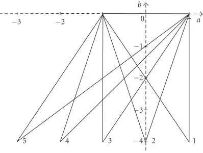
Figure 3.1. Stability diagram,σ0=0, differingθvalues.
b 0 10 9 8 7 6 5
4
3
2
1
−1
−2
−3
−4
−3
−2
−1
1 a
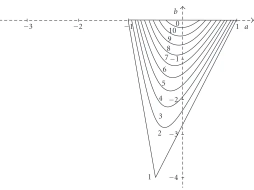
Figure 3.2. Stability diagram,θ=1, differingσ2 0 values.
or
θ−1
4
b−
1 +b 4
2 −σ2
0< a <
θ−1
4
b+
1 +b 4
2 −σ2
0, −4
1−σ0< b≤0. (3.34)
Stability regions, obtained by virtue of condition (3.34) forσ0=0 and different values of
b
Stability regions, obtained by virtue of condition (3.34) forθ=1 and different values ofσ02are shown inFigure 3.2with the following key: (1)σ02=0, (2)σ02=0.1, (3)σ02= 0.2, (4)σ2
0=0.3, (5)σ02=0.4, (6)σ02=0.5, (7)σ02=0.6, (8)σ02=0.7, (9)σ02=0.8, (10)
σ2
0 =0.9.Figure 3.3uses the same key asFigure 3.2and is forθ=0.375.
Remark 3.1. Note that the stability region, given by condition (3.34) depends onθand σ0, but the areaSof this stability region depends onσ0only and does not depend onθ,
Stability condition (3.34) in the terms of initial equation (1.1) takes the form
11
10
9
8
7
6 5
4
3 2
1
5 4 3
−1500
−1000
−500 α β
−75 −50 −25
−100 1
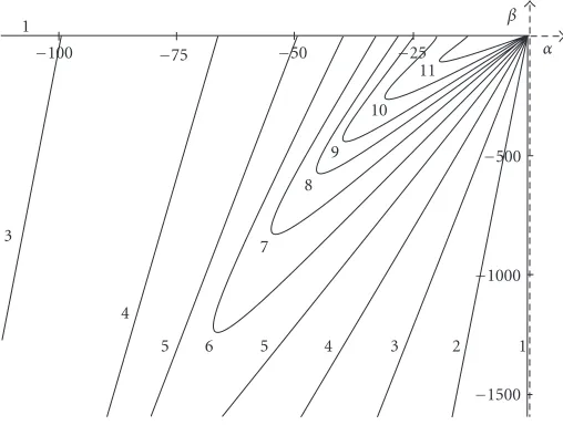
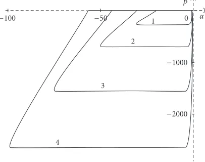
Figure 3.4. Stability diagram,θ=1,σ2=0, differinghvalues.
11
10
9
8
7
6 5 4 3 2 1
5 4 3
−1500
−1000
−500 α β
−75 −50 −25
−100 1
Figure 3.5. Stability diagram,θ=1,σ2=1, differinghvalues.
The stability regions in the (α,β) space, obtained by condition (3.37) forθ=1,σ2=0 are shown inFigure 3.4for different values of the step sizehof the numerical method, using the following key: (1)h=0, (2)h=0.01, (3)h=0.02, (4)h=0.03, (5)h=0.04, (6)h=0.05, (7)h=0.06, (8)h=0.07, (9)h=0.08, (10)h=0.1, (11)h=0.15. Figures
3.5and3.6show similar pictures withθ=1 andhas indicated above but withσ2=1 and
11 10 9
8
7
6
5 4 3 2 1
5 4 3
−1500
−1000
−500 α β −75 −50 −25
−100 1
Figure 3.6. Stability diagram,θ=1,σ2=3, differinghvalues.
5 4 3 2 1
−1500
−1000
−500 α β
−50 −25
Figure 3.7. Stability diagram,σ2=1,h=0.05, differingθvalues.
Figure 3.7illustrates the stability region in the (α,β) space forσ2=1,h=0.05 and different valuesθ(i.e., different numerical schemes) according to the following key: (1) θ=0, (2)θ=0.25, (3)θ=0.5, (4)θ=0.75, (5)θ=1.
If we calculate the infimum with respect toθin the left-hand part and the supremum in the right-hand part of inequalities (3.37) we obtain
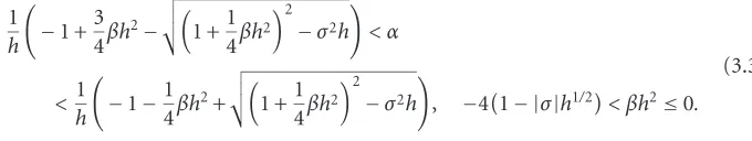
1 h
−1 +3 4βh
2−
1 +1 4βh
2
2 −σ2h
< α
<1 h
−1−1
4βh 2+
1 +1 4βh
2
2 −σ2h
, −41− |σ|h1/2< βh2≤0.
4
3
2
1 −300
−200
−100 α β
−30 −20 −10 0
Figure 3.8. Stability diagram,h=0.1, differingσ2values.
4
3 2
1 0
−1000
−2000
−100 −50 α
β
Figure 3.9. Stability diagram,σ2=1, differinghvalues.
It is easy to check that ifh→0 then condition (3.38) coincides with condition (2.16). It leads to the following useful statement.
Theorem3.2. Ifα,βandσ satisfy condition (2.16) then there exists a small enoughhsuch that condition (3.38) holds too. And ifα,β,σandhsatisfy condition (3.38) then there exists aθ∈[0, 1]such that condition (3.37) holds too and therefore the trivial solution of (3.1) is asymptotically mean square stable.
The stability regions obtained by condition (3.38) forh=0.1 and different values of σ are shown inFigure 3.8, according to the following key: (1)σ2=0.5, (2)σ2=1, (3)
5 4 3 2 1
−1500
−1000
−500 0 α β
−50 −25
B2 B1
E1
E2 C1
C2 D2 D1
A1 A2
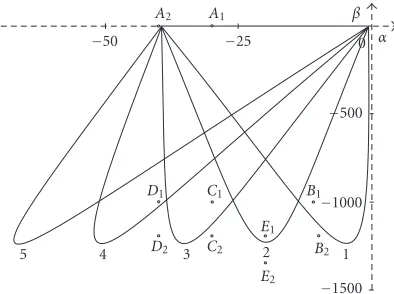
Figure 4.1. Stability diagram,σ2=1,h=0.05, differingθvalues.
4. Upper bound for the step of discretization
From condition (3.37) it follows that f(h)>0 where
f(h) :=θ
θ−1
2
β2h3−
2θ−1
2
αβh2+α2−2βθh+ 2α+σ2. (4.1)
Using the representation (4.1) consider different possible cases for determining an upper bound for the step of discretization.
4.1. Caseβ=0. Let β=0. From (4.1), (2.16) we obtain f(h)=α2h+ 2α+σ2<0 for
h∈[0,h1), where
h1= −2α+σ 2
α2 >0. (4.2)
For example, if α= −30, β=0,σ2=1 then h
1≈0.0656. Changingα toα= −40, we obtainh1≈0.0494. OnFigure 4.1which coincides withFigure 3.7(σ2=1,h=0.05) the pointsA1(−30, 0) andA2(−40, 0) are shown. One can see that the pointA1belongs to the stability region but the pointA2does not belong sinceh=0.05> h1=0.0494.
Suppose now thatβ <0 and consider the following possibilities forθ.
4.2. Caseθ=0. Letθ=0. Then
f(h)=1 2αβh
2+α2h+ 2α+σ2. (4.3)
Since 2α+σ2<0 andαβ >0 then f(h)<0 forh∈[0,h
1), where
h1=
α4−2αβ2α+σ2−α2
For example, ifα= −10,β= −1000,σ2=1 thenh
1≈0.0524. Changingβtoβ= −1200 we obtain h1≈0.0486<0.05. OnFigure 4.1 the pointB1(−10,−1000) belongs to the stability region withθ=0 and the pointB2(−10,−1200) does not belong.
4.3. Caseθ=1/2. Letθ=1/2. Then
f(h)= −1
2αβh 2+
α2−βh+ 2α+σ2. (4.5)
Since
D=α2−β2+ 2αβ2α+σ2)=α2+β2+ 2αβσ2>0 (4.6)
then f(h)<0 forh∈[0,h1), where
h1=α
2−β−√D
αβ >0. (4.7)
For example, ifα= −30,β= −1000,σ2=1 thenh
1≈0.0545. Changingβonβ= −1200 we obtainh1≈0.0472. On Figure 4.1the point C1(−30, 1000) belongs to the stability region withθ=1/2 and the pointC2(−30,−1200) does not belong to this region.
4.4. Caseθ∈(1/2, 1]. Letθ∈(1/2, 1]. From (4.1) and (2.16) it follows that f(h)<0 for h≤0. So f(h)<0 forh∈[0,h1), whereh1is the least root of the equation f(h)=0. For example, ifα= −40,β= −1000,σ2=1,θ=0.75 we obtain
f(h)=187500h3−40000h2+ 3100h−79=0 (4.8)
andh1≈0.0511. Changingβtoβ= −1200 we obtain
f(h)=270000h3−48000h2+ 3400h−79=0 (4.9)
withh1≈0.0431. OnFigure 4.1the pointD1(−40,−1000) belongs to the stability region withθ=3/4 but the pointD2(−40,−1200) does not belong to this region.
4.5. Caseθ∈(0, 1/2). Letθ∈(0, 1/2). From (4.1) and (2.16) it follows thatf(0)<0 and (df /dh)(0)>0. It means that f(h)<0 forh∈[0,h1) whereh1is the least positive root of the equation f(h)=0. For example, ifα= −20,β= −1200,σ2=1,θ=1/4 then
f(h)= −90000h3+ 1000h−39 (4.10)
andh1≈0.0508. Changingβtoβ= −1300 we obtain
f(h)= −105625h3+ 1050h−39=0 (4.11)
10 9 8 7 6 5 4 3 2 1 0
−2.5
−2
−1.5
−1
−0.5 0 0.5 1 1.5 2 2.5
τ=ih
Xt
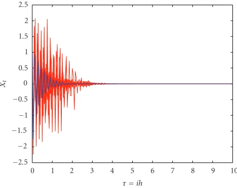
Figure 5.1. Trajectories of (3.1) withm=0,α= −55,β= −1000,σ2=1,h=0.05,θ=1,x 0=1.
10 9 8 7 6 5 4 3 2 1 0
−2
−1.5
−1
−0.5 0 0.5 1 1.5×10
13
τ=ih
Xt
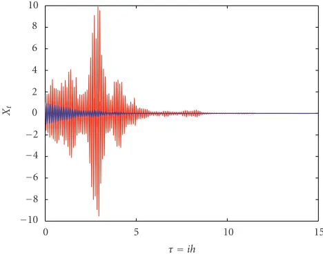
Figure 5.2. Trajectories of (3.1) withm=0,α= −55,β= −1000,σ2=1,h=0.06,θ=1,x 0=1.
5. Numerical experiments
We illustrate some of our results with trajectories of (3.1). Note that in [30] an absolute correspondence of asymptotic mean square stability of the trivial solution and conver-gence of trajectories to zero was shown.
10 9 8 7 6 5 4 3 2 1 0
−2500
−2000
−1500
−1000
−500 0 500 1000 1500 2000 2500
τ=ih
Xt
Figure 5.3. Trajectories of (3.1) withm=0,α= −40,β= −25,σ2=1,h=0.05,θ=0,x 0=1.
15 10
5 0
−10
−8
−6
−4
−2 0 2 4 6 8 10
τ=ih
Xt
Figure 5.4. Trajectories of (3.1) withm=0,α= −40,β= −25,σ2=1,h=0.05,θ=1,x 0=1.
system. If we change the parameterhtoh=0.06 we no longer have a stable system (as shown inFigure 5.2, as expected from examiningFigure 3.5).
20 18 16 14 12 10 8 6 4 2 0
−300
−200
−100 0 100 200 300
τ=ih
Xt
Figure 5.5. Trajectories of (3.1) withm=0,α= −40,β= −25,σ2=1,h=0.05,θ=0.5,x 0=1.
20 18 16 14 12 10 8 6 4 2 0
−4
−3
−2
−1 0 1 2 3 4 5
τ=ih
Xt
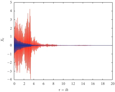
Figure 5.6. Trajectories of (3.1) withm=0,α= −39,β= −25,σ2=1,h=0.05,θ=0,x 0=1.
which replicates this stability property. InFigure 5.3the sufficient conditions for asymp-totic mean square stability of the discrete system (i.e., −38.8603< α <−0.5147, given the other parameters) are not satisfied and the trajectories are indeed unstable, whereas in Figures 5.4and 5.5the conditions (i.e., −40.1103< α <−1.7647 forFigure 5.4and
−39.4853< α <−1.1397 forFigure 5.5, given the other parameters) are satisfied and we have asymptotic mean-square stability.Figure 5.6uses the same parameters asFigure 5.3
square stability, thus verifying that are conditions are only sufficient and not necessary and sufficient. However we believe our experiments indicate that the sufficient condi-tions are very good ones.
Acknowledgments
This work has been completed with the financial assistance of NATO, grant reference PST.EV.979727, to whom the authors wish to express their thanks. We would also like to thank Dr John Edwards and Prof Neville Ford of University College Chester for helpful comments relating to early drafts of the work.
References
[1] V. N. Afanas’ev, V. B. Kolmanovskii, and V. R. Nosov,Mathematical Theory of Control Systems Design, Mathematics and Its Applications, vol. 341, Kluwer Academic, Dordrecht, 1996. [2] H. Brunner and J. D. Lambert, Stability of numerical methods for Volterra integro-differential
equations, Computing (Arch. Elektron. Rechnen)12(1974), no. 1, 75–89.
[3] H. Brunner and P. J. van der Houwen,The Numerical Solution of Volterra Equations, CWI Mono-graphs, vol. 3, North-Holland, Amsterdam, 1986.
[4] S. Busenberg and K. L. Cooke, The effect of integral conditions in certain equations modelling epidemics and population growth, Journal of Mathematical Biology10(1980), no. 1, 13–32. [5] A. Drozdov, Explicit stability conditions for stochastic integro-differential equations with
non-selfadjoint operator coefficients, Stochastic Analysis and Applications17(1999), no. 1, 23–41. [6] J. T. Edwards, N. J. Ford, and J. A. Roberts,The numerical simulation of the qualitative behaviour
of Volterra integro-differential equations, Proceedings of Algorithms for Approximation IV (Hud-dersfield, 2001) (J. Levesley, I. J. Anderson, and J. C. Mason, eds.), University of Hud(Hud-dersfield, Huddersfield, 2002, pp. 86–93.
[7] J. T. Edwards, N. J. Ford, J. A. Roberts, and L. E. Shakhet,Stability of a discrete nonlinear integro-differential equation of convolution type, Stability and Control: Theory and Applications. An In-ternational Journal3(2000), no. 1, 24–37.
[8] S. Elaydi and S. Sivasundaram,A unified approach to stability in integrodifferential equations via Liapunov functions, Journal of Mathematical Analysis and Applications144(1989), no. 2, 503– 531.
[9] N. J. Ford, C. T. H. Baker, and J. A. Roberts,Nonlinear Volterra integro-differential equations— stability and numerical stability ofθ-methods, Journal of Integral Equations and Applications10 (1998), no. 4, 397–416.
[10] I. I. Gihman and A. V. Skorokhod,Stochastic Differential Equations, Izdat. Naukova Dumka, Kiev, 1968.
[11] J. Golec and S. Sathananthan,Sample path approximation for stochastic integro-differential equa-tions, Stochastic Analysis and Applications17(1999), no. 4, 579–588.
[12] ,Strong approximations of stochastic integro-differential equations, Dynamics of Contin-uous, Discrete & Impulsive Systems. Series B. Applications & Algorithms8(2001), no. 1, 139– 151.
[13] D. J. Higham, X. R. Mao, and A. M. Stuart,Strong convergence of Euler-type methods for nonlinear stochastic differential equations, SIAM Journal on Numerical Analysis40(2002), no. 3, 1041– 1063.
[14] ,Exponential mean-square stability of numerical solutions to stochastic differential equa-tions, LMS Journal of Computation and Mathematics6(2003), 297–313.
[16] V. B. Kolmanovskii and A. Myshkis,Applied Theory of Functional-Differential Equations, Math-ematics and Its Applications (Soviet Series), vol. 85, Kluwer Academic, Dordrecht, 1992. [17] V. B. Kolmanovskii and L. E. Shaikhet,A method for constructing Lyapunov functionals for
sto-chastic systems with aftereffect, Differentsial’nye Uravneniya29(1993), no. 11, 1909–1920, 2022 (Russian), translation in Differential Equations29(1993), no. 11, 1657–1666 (1994).
[18] ,New results in stability theory for stochastic functional-differential equations (SFDEs) and their applications, Proceedings of Dynamic Systems and Applications, Vol. 1 (Atlanta, GA, 1993), Dynamic, Georgia, 1994, pp. 167–171.
[19] ,A method for constructing Lyapunov functionals for stochastic differential equations of neutral type, Differentsial’nye Uravneniya31(1995), no. 11, 1851–1857, 1941, translation in Differential Equations31(1995), no. 11, 1819–1825 (1996).
[20] ,General method of Lyapunov functionals construction for stability investigation of stochas-tic difference equations, Dynamical Systems and Applications, World Sci. Ser. Appl. Anal., vol. 4, World Scientific, New Jersey, 1995, pp. 397–439.
[21] ,Construction of Lyapunov functionals for stochastic hereditary systems: a survey of some recent results, Mathematical and Computer Modelling36(2002), no. 6, 691–716.
[22] ,Some peculiarities of the general method of Lyapunov functionals construction, Applied Mathematics Letters. An International Journal of Rapid Publication15(2002), no. 3, 355–360. [23] ,About one application of the general method of Lyapunov functionals construction,
Inter-national Journal of Robust and Nonlinear Control13(2003), no. 9, 805–818, Special issue on Time-Delay Systems, RNC.
[24] J. D. Lambert,Numerical Methods for Ordinary Differential Systems: The Initial Value Problem, John Wiley & Sons, Chichester, 1991.
[25] J. J. Levin and J. A. Nohel,Note on a nonlinear Volterra equation, Proceedings of the American Mathematical Society14(1963), 924–929.
[26] X. R. Mao,Stability of stochastic integro-differential equations, Stochastic Analysis and Applica-tions18(2000), no. 6, 1005–1017.
[27] B. Øksendal,Stochastic Differential Equations: An Introduction with Applications, 5th ed., Uni-versitext, Springer, Berlin, 1998.
[28] Y. Saito and T. Mitsui,Stability analysis of numerical schemes for stochastic differential equations, SIAM Journal on Numerical Analysis33(1996), no. 6, 2254–2267.
[29] L. E. Shaikhet,Necessary and sufficient conditions of asymptotic mean square stability for stochas-tic linear difference equations, Applied Mathematics Letters. An International Journal of Rapid Publication10(1997), no. 3, 111–115.
[30] ,Numerical simulation and stability of stochastic systems with Markovian switching, Neu-ral, Parallel & Scientific Computations10(2002), no. 2, 199–208.
[31] ,About Lyapunov functionals construction for difference equations with continuous time, Applied Mathematics Letters. An International Journal of Rapid Publication17(2004), no. 8, 985–991.
[32] ,Construction of Lyapunov functionals for stochastic difference equations with continuous time, Mathematics and Computers in Simulation66(2004), no. 6, 509–521.
[33] ,Lyapunov functionals construction for stochastic difference second-kind Volterra equations with continuous time, Advances in Difference Equations2004(2004), no. 1, 67–91.
Leonid E. Shaikhet: Department of Higher Mathematics,
Donetsk State University of Management, Donetsk 83015, Ukraine
E-mail address:[email protected]
Jason A. Roberts: Mathematics Department, University of Chester, Chester CH14BJ, England