R E S E A R C H
Open Access
A unified framework for adaptive inverse
power control
Marko Höyhtyä
*and Aarne Mämmelä
Abstract
In this paper, a unified framework for adaptive inverse power control is developed. It is based on a modified filtered-x least mean square (MFxLMS) algorithm that is proposed and analyzed. A practical version of the algorithm for closed loop power control is also developed. The filtered-x least mean square (FxLMS) algorithm is widely used for inverse control such as noise cancelation. This is the first paper to apply the algorithm for power control. We have modified the conventional FxLMS algorithm by adding absolute value blocks since power control does not need phase information. The modification makes the algorithm more robust and requires fewer bits to be transmitted in the feedback link. The main contribution of the paper is that the proposed algorithm can be seen as generalized inverse control to be used in power control research. It gives a unified framework for several existing algorithms, linking them to the least mean square (LMS) literature. Numerical results are provided, comparing the performance of the proposed algorithm to existing practical algorithms used, e.g., in Third Generation Partnership Project (3GPP) long-term evolution (LTE) systems.
Keywords:Power control, Feedback control systems, Adaptive signal processing
1 Introduction
Inverse control has been used for several applications such as channel equalization [1, 2] automatic gain con-trol (AGC) [3], noise and interference cancelation [4, 5], and transmission power control [6, 7] which is the topic of this paper. Due to stability problems, the least mean square (LMS) algorithm is not directly suitable for active control applications where the adaptive filter works as a controller for a time-variant system. Instead, the filtered-x least mean square (Ffiltered-xLMS) algorithm is a good choice for that kind of applications [4]. It is essentially the LMS algorithm with a few little changes so that algorithm can remain stable. The FxLMS algorithm is developed from the LMS algorithm by inserting the model of the controlled system between the input data signal and the adaptive algo-rithm that updates the coefficients of adaptive filter. The algorithm was introduced independently in [8, 9] and [10] for adaptive control and noise cancelation.
Conventionally, power control research and LMS algorithm research have been advanced in separate paths. We propose and demonstrate a new use of the FxLMS
algorithm in this article, namely power control. This inte-grates previously separated paths, providing unified frame-work for adaptive inverse power control.
We described the FxLMS method initially for power control in [11] and compared it by numerical simula-tions to other practical algorithms in [11] and [12]. We developed also a truncated version of the algorithm in [13] to improve energy efficiency. Truncation means that the transmission is interrupted and transmission power is zero when the magnitude of the channel gain deterio-rates under a certain cutoff value. Since transmission power control is a new application for the algorithm, new phenomena occur and modifications are needed. Fading in the wireless channel has a wide dynamic range, and changes are fast compared to conventional control systems. In addition, wireless feedback channel limits the number of bits used in control commands. We have modified the conventional FxLMS algorithm by adding absolute value blocks since power control does not need phase information. The modification makes the algorithm more robust and requires fewer bits to be transmitted in the feedback link.
In this paper, we show with analysis that the proposed algorithm converges exactly to the wanted solution in a
* Correspondence:marko.hoyhtya@vtt.fi
VTT Technical Research Centre of Finland Ltd, P.O. Box 1100, FI-90571 Oulu, Finland
noiseless channel. We restrict our investigation purely to the closed loop part, focusing on the algorithm and thus assuming ideal feedback. Simulations show that the algo-rithm converges well also in a noisy channel. The main contribution of this paper compared to our previous pa-pers is that we create a unified framework for inverse power control for cellular systems. The proposed algo-rithm links the existing algoalgo-rithms to LMS type of adap-tive algorithms. The modified filtered-x least mean square (MFxLMS) algorithm can be seen as a generalized adaptive inverse control method and several practical algorithms as special cases of it. In addition to theoretical analysis that is made more thoroughly in this paper than in our previous papers, we develop a practical quantized version of the al-gorithm and compare its performance to state-of-the-art algorithms. The proposed algorithm provides a fast adapt-ing inverse power control solution that does not overshoot the power level as much after a fade as the conventional solution in [14]. Thus, it decreases interference to other users in these cases. We also propose an efficient way to implement the closed loop algorithm described in [15] as an enhanced version of the algorithm presented in [14].
Furthermore, we present novel fast simulation models for a fading channel and diversity. It was reported in [16] that Jakes’model [17] does not produce wide-sense stationary signals. The authors of [16] proposed to im-prove the model by randomizing the phase shifts of the low-frequency oscillators. We have modified Jakes’model further by randomizing also the frequency shifts in the model. Several simulation studies are performed with the practical power control algorithms both in additive white Gaussian noise (AWGN) and fading channels. The model is applicable to a multiple-input multiple-output orthog-onal frequency division multiplexing (MIMO-OFDM) sys-tem with certain assumptions as discussed in Section 3. MIMO FxLMS algorithm has been recently studied for vi-bration control in [18].
The organization of the paper is as follows. Section 2 discusses related literature, and Section 3 presents the system model. Performance metrics are introduced in Section 4. The MFxLMS algorithm with the convergence analysis is presented with several other adaptive inverse power control schemes in Section 5. Achieved results are provided in Section 6, and conclusions with recom-mendations for further work are drawn in Section 7.
2 Related literature
Power control methods can in general be divided into water filling and channel inversion [6]. Basically, the difference between these two approaches is that the water filling allocates more power to the better channel instants whereas channel inversion aims at inverting the channel power gain while maintaining the desired signal strength at the receiver.
Several adaptive inverse control methods have been developed and studied in the literature for power con-trol, e.g., [14, 15, 19–24]. The conventional 1-bit adap-tive power control (CAPC-1) method [14, 19] employs delta modulation, i.e., adjusts the previous transmission power up or down by a fixed step. In this paper, the
acronym CAPC-x refers to conventional power control
using x bits in the power control command.
Conven-tional inverse power control approaches have been pro-posed and used, e.g., for code division multiple access (CDMA), Third Generation Partnership Project (3GPP) long-term evolution (LTE), and TV white space trans-mission. A clear aim of these inverse methods is energy and interference reduction, to use only sufficient power to meet the transmission rate requirements. For example, CDMA power control employs both closed and open loop methods. In the open loop method, the mobile station mea-sures the average received total power by an automatic gain control (AGC) circuit and adjusts its transmission power so that it is inversely proportional to the received power [25]. Nonlinear control is used to allow fast response to the re-duced channel attenuation with a maximum of 10 dB/ms but slow response to increased attenuation. This is to avoid additional interference to other users.
Required dynamic range with a limited feedback can be achieved by nonlinear quantization of feedback signal-ing [26] and variable step (VS) algorithms [27–30]. Non-linear AGC control can be exponential or approximately exponential [3]. A simple way to compress power control commands is to operate the algorithm in decibel domain [20]. Logarithmic quantization such as μ-law and A-law companding is used in speech codecs [26]. Companding amplifies weak input signals and compresses strong sig-nals to save the needed number of bits to be transmitted. Companding is applied also for reducing peak-to-average power ratio (PAPR) in OFDM signals [31].
Many variable step size LMS algorithms have been pro-posed in order to improve the performance of the LMS al-gorithm by using large step sizes in the early stages of the adaptive process and small step sizes when the system
ap-proaches convergence [27–30]. The step size can be
adapted, e.g., based on the received signal power [11] or the squared error signal [19, 20]. Optimization of the step size has been studied in [32], where lag error of an adap-tive system is also considered. This error is caused by the attempt of an adaptive system to track variations of the non-stationary input signal.
3 System model
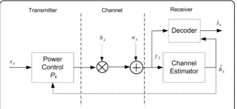
The system model for adaptive transmission is illustrated in Fig. 1. The input dataxkare binary phase-shift keying
PSK and M-ary quadrature amplitude modulation (QAM) without any modifications. On the other hand, the analysis for each modulation scheme must be con-sidered separately. The analysis for quadrature phase-shift keying (QPSK) is essentially the same since QPSK can be viewed as two independent BPSK signals in a
frequency-nonselective channel. The received signal yk
can be given as.
yk¼xkPkhkþnk: ð1Þ
The complex gain of the channel is hk ¼ αkejθk and
nk is the additive white Gaussian noise at time k. The
amplitude of the fading gain is αk and θk is the phase
shift. The data are transmitted through the channel and
the instantaneous transmit power Pk is allocated based
on the channel gain estimate ĥk sent by the receiver. LMS estimation of the channel gain is done as.
ĥkþ1¼ĥkþϑekxk ð2Þ
whereϑis the step size of the algorithm andekis the
estima-tion error [1]. A typical value for the step sizeϑis 0–0.99. Lar-ger values lead to faster convergence with the cost of reduced accuracy since noise averaging does not work so well [33].
We consider a slowly varying channel that can be modeled using the Doppler power spectrum [16, 17]. The rate of the channel variation, i.e., the effect of mo-bility, can be characterized by the Doppler frequency fd.
We are using a flat Doppler power spectrum that corre-sponds to an urban environment where the transmitter is set above rooftop level [34].
3.1 Sum-of-sinusoids fading channel
To obtain a flat Doppler power spectrum, the time-variant channel gain of a channel with indexl is repre-sented by the sum of complex exponentials as.
hlðkÞ ¼
where N is the number of subpaths with the same
delay,fi,lis the Doppler shift of the ith subpath,i,lis the
random phase shift of theith subpath uniformly distrib-uted in the range [0, 2π], and kis the time. The ampli-tudes of the subpaths in Eq. (3) are identical due to the flat spectrum. The average energy gain of the channel is normalized to unity [35]. The model is straightforward to generalize to multiple delays.
If the Doppler shifts of the complex exponentials are equally spaced in the interval [−fd, fd], the channel gain
(Eq. (3)) becomes periodic in time. Sampling in time do-main corresponds to periodicity in frequency dodo-main and vice versa [36]. Periodicity can be removed if the shifts are properly chosen. The Doppler spread is divided into Nequal size frequency bins. Within these bins, the frequencies fi,l differ a random uniformly distributed
amount from the equal space solution. Thus, we obtain the whole Doppler spread to use in every simulation. The power spectrum is made symmetric with respect to zero frequency, which makes the autocorrelation func-tion of the channel real. This selecfunc-tion also makes simu-lations faster. The random phasesϕi,lare not symmetric
with respect to the zero frequency.
3.2 Diversity channel
A time-variant frequency selective channel model can be represented with a tapped delay line as.
βð Þ ¼l;k 1
delay of lth tap generated using Eq. (3). Now, we have a flat impulse response instead of usual exponentially de-creasing model. However, from power control point of view, this does not affect since the optimal demodulator for this signal is a coherent demodulator that collects the signal energy from all the received signal paths within the delay span 0 to τL[2]. In a diversity system,
the transmitter power control algorithm should control the power of the diversity combiner output in the re-ceiver. There is no loss in performance in dividing the
total transmitted signal energy differently among the L
channels, and thus, the model does not change the com-parison between the selected power control algorithms. Actually, the time-variant channel gain of the diversity channel can be given as.
H kð Þ ¼
branch, generated using Eq. (3), andL is the number of
diversity branches. Equation (5) corresponds to the ideal maximal-ratio combining. The channel can thus repre-sent also a frequency selective channel. From the
subcarrier point of view, frequency selective channel looks frequency-nonselective in an OFDM system [2]. We assume that no intersymbol interference (ISI) or interpulse interference (IPI) is present since we use
com-pressed pulses [2]. In general, a MIMO system with Mt
transmitter antennas and Nr receiver antennas can be
used as a diversity system having Mt×Nr independent
diversity branches [37]. With OFDM system, those branches are made frequency-nonselective, and finally, by the use of orthogonal codes, the branches can be sep-arated from each other. The channel must be slowly fad-ing compared to the OFDM symbol rate so that intercarrier interference is avoided. The fading of the ad-jacent subcarriers is not uncorrelated, but this is typical in all OFDM systems, and it is in practice handled with frequency domain interleaving. Thus, with these as-sumptions, our system model represents also a MIMO-OFDM system.
4 Performance metrics
Suitable performance metrics are needed to fairly compare the performance of the adaptive algorithms. One of the most important ones to consider is the signal-to-noise ratio (SNR) concept. The average transmitted and the average received energies are usually normalized by the receiver noise spectral
density N0 leading to the average transmitted SNR
per symbol [35].
γtx¼Etx=N0 ð6Þ
and the average received SNR per symbol [35]
γrx¼Erx=N0: ð7Þ
The parameter Ētx is the average transmitted energy
per symbol, and Ērx is the average received energy per
symbol. Transmitted energy is a basic system resource. In a mobile terminal, it is taken from the battery of the transmitter and is therefore limited. Transmitted energy or equivalently transmitted SNR should be used as a performance metric in order to obtain fair comparisons between different adaptive transmission systems. In adaptive transmission, the transmitted signal is a func-tion of the energy gain of the channel. The use of the re-ceived SNR as a performance criterion in adaptive transmission system studies can lead to misleading re-sults as was shown in [35].
Learning curve, i.e., plotting the mean square error (MSE) against the number of iterations, can be used to measure the statistical performance of adaptive algo-rithms [1, 2]. The MSEJ(k) can be approximated as.
where εk is the error signal measured as a difference
between the output of the adaptive algorithm and the
desired signal. Parameter η defines the number of
sam-ples used for averaging. Usually, MSE is compared to signal power, in this case transmission power.
5 Adaptive power control methods
5.1 Theoretical inverse control methods
If the truncated channel inversion (TCI) is used, the transmitted energy is [38].
Etxð Þ ¼k Etxðσ0=γHð Þk Þ ð9Þ
for γH(k) ≥ γ0 and zero otherwise where σ0is a
con-stant selected so that the average transmitted energy is
Ētx. The quality of the channel is defined as γH(k) = Ētx|H(k)|2/N0, γ0,γ0is a cutoff value, which is found by
numerically maximizing (4.22) in [38], and |H(k)|2is the instantaneous energy gain of the channel. The cutoff value isγ0= 0 for full channel inversion. Channel
inver-sion aims at maintaining the desired signal strength at the receiver by inverting the channel power gain based on the channel estimates.
5.2 Adaptive FxLMS algorithm
The power control structure based on the MFxLMS al-gorithm is introduced in Fig. 2. It approximates the channel inversion. In the following, we will present both original and modified versions of the algorithm. The FxLMS algorithm updates the coefficientckof a one-tap
filter as.
ck¼ck−1þwk ð10Þ
where wk¼μx
0
kεk is the correction term, μ is the adaptation step size of the algorithm that regulates the speed and stability of adaptation, and εkis the error
sig-nal to be minimized. The ck is the instantaneous
trans-mission power at a time slotk. The filtered input signal for the FxLMS algorithm is x0k¼ x̂kĥk
, where x* is the complex conjugate version of x, x̂k is the estimated input signal, andĥk is the estimated instantaneous chan-nel gain. The filtered input signal is x0k¼ x̂kĥk for
the MFxLMS algorithm, and the parameter nk is the
additive white Gaussian noise. The channel can be modeled using Eqs. (3)–(5).
to conventional control systems comes with a separate re-ceiver and transmitter. The main reason for the addition of absolute value blocks is that we are adjusting power levels and thus interested only in amplitude values, similar to AGC circuits [3]. Phases are not important from the power control point of view, and in this way, we can reduce control information to be carried. This also makes the system more robust since phases can change fast during deep fades and thus cause problems to the adaptive algorithm [39, 40].
The model is discretized using a matched filter [2], as-suming slow changes compared to the symbol rate. Thus, we can use one sample of a symbol in the system model. We can reduce the complexity of the transmitter by doing the main part of the calculations at the receiver. This re-duces also information in the feedback channel since only the correction termwk is sent to the transmitter. The
fil-tered input signalx0kaffects the operation of the algorithm. Thus, the control structure is decision directed (DD) [2]. Error propagation is known in DD approaches and remedy strategies have been developed [41, 42]. It was proposed in [42] that pilot on request training (PRQT) is used to miti-gate the error propagation. The pilot is requested when error propagation is detected in the system. We assume our system to operate with the PRQT principle. When the error probability is very small, we can assumex̂kto bexk.
5.2.1 Convergence analysis for the MFxLMS power control algorithm
The choice of initial conditions for the FxLMS algorithm is not critical [4]. The algorithm is stable if μ is small
enough, and transients die out just as with the conven-tional LMS algorithm. A primary concern with the MFxLMS algorithm is its convergence to the optimal
so-lution where E ε2k is minimized. Since absolute value
blocks make the analysis of the algorithm very compli-cated in a noisy channel, we will first analyze the con-ventional FxLMS algorithm that can also be used in power control. A general analysis for the FxLMS algo-rithm can be found in [43].
(a)Coherent case
Let us assume a time-invariant channel with perfect channel estimation, i.e.,ĥk ¼h. The error signal is now
εk¼xk−ðhck−1xkþnkÞ: ð11Þ
The control command (Eq. (10)) can be given as
ck¼ck−1þðxkhÞμεk; ð12Þ
and placing error signal (Eqs. (11) to (12)) yields
ck¼ck−1 1−μj jh2j jxk2
þμhj jxk2−μhxknk: ð13Þ
Taking expected value of both sides leads to
E c½ ¼k 1−μj jh2R
E c½ k−1 þμhR ð14Þ
where R=E[|xk|2]. The white noise nk is assumed to
be uncorrelated with the input xk. In addition, we
as-sume that the inputxkis independent of the weightckas
in the analysis of the LMS algorithm in [4]. The first part
of the function in the right-hand side will clearly form a geometric series that will converge only if the geometric ratio has a magnitude of less than unity,
1−μj jh2R
Since the first part of the sum in Eq. (16) will ap-proach zero, the algorithm converges exactly to the in-verse of the channel gain. We can see from Eq. (15) that in order to keep the algorithm stable, the step size for updating the algorithm coefficients should be
0<μ< 2
R hj j2: ð17Þ
The optimal step size for the FxLMS algorithm lies in the middle of stability interval [43, 44]. The convergence will be fastest with this selection. Thus, the optimal step size is now
μopt ¼ 1
R hj j2: ð18Þ
With this selection, the fixed step FxLMS algorithm is changed to the normalized version of it.
(b)Non-coherent case
From the power control point of view, we would only need the inverse of the absolute value of the channel gain instead of the result of Eq. (16) since we are interested in inverting the power level to maintain the received signal power at a constant level. Thus, let us now consider the MFxLMS algorithm with absolute value blocks in a time-invariant, noiseless channel, assuming perfect channel es-timation, i.e.,ĥk¼h. The error signal is given as
εk¼j j−xk jhck−1xkj: ð19Þ
Thus, Eq. (10) becomes
ck¼ck−1þμj jh2j jxk2−μjck−1jj jxk2j jh: ð20Þ
In general, we should consider two separate cases:ck>
0 and ck< 0. However, there is no need to use negative
values in power control since the solution we want to achieve is to maintain certain SNR at the receiver. The caseck< 0 leads to the converged solution that is a
nega-tive version of the solution for the case ofck> 0. When ck> 0, |ck| =ck. Now,
ck¼ 1−μj jxk2j jh2
ck−1þμj jxk2j jh: ð21Þ
Convergence conditions for the MFxLMS algorithm can be found from this version quite straightforwardly, leading to the same solution as is shown in Eq. (15). Therefore, we can write
c∞¼ 1 h
j j; ck>0: ð22Þ
The algorithm converges exactly to the inverse of the absolute value of the channel gain. We can see from the results above that in order to keep the algorithm stable, the step size for updating the algorithm coefficients should be exactly in the same interval as the one shown in Eq. (17). Thus, the optimal step size for the MFxLMS algorithm in a noiseless channel is given in Eq. (18).
Convergence of the MFxLMS algorithm when noise is present in the system becomes mathematically intract-able due to the absolute value blocks. Now, Eq. (10) can be rewritten as
ck¼ck−1þμj jhj jxk2−μjhxkjjhxkck−1þnkj: ð23Þ
The algorithm cannot be analyzed straightforwardly due to absolute value of the term that includes noise. Simulations are also used instead of analysis in reference state-of-the art algorithm developments due to mathem-atical intractability [14, 15, 19–21]. Based on the simula-tions, the MFxLMS algorithm behaves and converges almost identically with the algorithm without absolute blocks in a fading channel when the transmitted SNR is high enough. Actually, the MFxLMS algorithm is more robust since fast phase changes do not affect its per-formance. Nonlinearity causes threshold phenomenon for the modified algorithm in low SNR regime that is al-ways a problem in noncoherent systems using some combining or averaging.
5.2.2 Time-variant channel
Usually, the adaptation step size of the FxLMS algorithm is not time variant. The algorithm with a fixed adapta-tion step size corresponds to a first-order system. It can-not track the fastest changes in the time-variant channel without a lag error [32] that can be quite large. A better performance is achieved by optimizing the adaptation step size with the instantaneous power of the input sig-nal. It means that the FxLMS algorithm with a fixed step size is changed to the normalized version of it. The nor-malized version of the FxLMS algorithm corresponds to the filtered-x recursive least squares (FxRLS) algorithm
when μ = 1−λ where λ is the forgetting factor which
gives exponentially less weight to older samples.
In a slowly fading channel,hkcan be assumed to be
Thus, the stability condition to the structure when noise is ignored and the channel state is known is the same as pre-sented in Eq. (17) whenhis replaced by hk. The optimal
step size can be found for each differenthkin Eq. (18) by
replacingh byhk. Therefore, the optimal adaptation step
size should be time variant. When the channel gain is esti-mated in Eq. (18), the system becomes unstable if this step size is used due to errors in the estimate [45]. To stabilize the control, the step size is given by.
μs¼
a
R ĥk 2þb ð24Þ
wherebis a small real number that prevents the adap-tation step size to grow uncontrollably when the
esti-mated received power is close to zero. Parameters aand
bare dependent, e.g., on SNR andL, but the values need to be found experimentally to optimize the trade-off be-tween lag error and noise averaging for different channel dynamics. Default values for these parameters can be given asa¼1=pffiffiffiL and b¼0:2=γrxwhereγrxis the
re-ceived SNR defined in Eq. (7). Smaller a means slower
convergence, better noise averaging, and a larger lag error while the parameterbhas an opposite effect.
5.2.3 Quantized MFxLMS power control
In the following sections, only the MFxLMS algorithm is considered. In practice, the power control command has to be quantized while obtaining a decent performance.
In the case of the MFxLMS algorithm, the signalwkhas
to be fed back to the transmitter as shown in Fig. 2. It is good to quantize frequently occurring small values of the signal in more detail and then use coarser steps for the less frequent large signal levels to preserve needed information [26]. The signalwkis first compressed, then
quantized uniformly, and sent to the channel. The re-ceived signal is expanded to get close to the original ver-sion of the power control command.
The μ-law compression is defined for real input
signal wk as
vk¼F wð Þ ¼k sgnð Þwk
Vln 1þμqj jwk=V
ln 1þμq
: ð25Þ
where V is the peak magnitude of the input signal.
This is also a peak value of the output. A typical value
for the compression parameter μq is between 50 and
300. In our case, we have quantized the signal in the range [−1, 1] to be able to effectively combat the deep fades even though the average power of the signal vkis
roughly 0.1. The maximum value is close to unity during the deepest fades. We have not scaled the signal before quantization. If the signal is scaled up, the clipping is in-creased while the quantization noise is reduced. Scaling down reduces clipping but increases noise. Received quantized signalqkis expanded using
ŵk¼F−1ð Þqk
¼sgnð Þqk μV q
!
ej jqk ln 1ðþμqÞ=V−1
; 0≤j j≤qk 1: ð26Þ
The proposed practical version of our MFxLMS rithm allows fair comparison with other practical algo-rithms presented in the literature.
5.3 Conventional adaptive power control
Typically, the time interval between power control com-mands in CDMA systems is around 1 ms [14]. The method is shown in Fig. 3. The base station measures
the average received power over m symbols and
com-pares it to a reference signal to interference plus noise (SINR) level γref. As a result of a comparison, the base
station tells the mobile station to adjust its transmission
power upwards when the error signal δk is positive or
downwards with negative error by a control step sizeΔP. Practical CAPC-1 method [14, 19] uses 1 dB steps. The power control algorithm can be written as.
Pk¼Pk−1þCkΔP ½ dB ð27Þ
where the power control command is
Ck¼ þ−11;; δδk>0 k≤0 :
ð28Þ
The weakness of this fixed-step power control method is that it is too slow to track changes in a fading channel.
5.4 Variable step adjustment power control
Variable step power control methods have been pro-posed to overcome the weakness of the fixed-step solu-tion. The basic idea is that when the power of received signal is far from the desired, the control step is in-creased to reach the desired level faster. A recently pro-posed 2-bit version of the CAPC (CAPC-2) method is
described in [15] where power control command Ck
values are Ck= {−4, −1, 1, 4} (dB). In the mentioned
document [15], only step sizes are given. No rules how to use them in practice are included. Based on the simu-lation studies, we have conducted the following rule that was found to achieve a good performance:
Ck¼
the conventional adaptive power control (CAPC-3) pro-posed in [20] is
Variable step algorithms can be implemented with the structure depicted in Fig. 3. The only difference to the 1-bit CAPC method is in the quantization, i.e., more bits are used for power control commands in CAPC-2 and CAPC-3.
5.5 Comparison between the FxLMS and conventional algorithms
The idea to use the FxLMS algorithm started from the observation that analogy can be seen between the con-trol structure in Fig. 3 and the LMS algorithm. Actually, the conventional algorithms can be seen as a special case of the FxLMS algorithm. The following modifications are needed from the MFxLMS structure in Fig. 2 to the CAPC structure in Fig. 3: (1) First, the CAPC structure
uses square-law detection instead of envelope detection used in the MFxLMS structure. These have shown to provide comparable performance but the former is usu-ally easier to analyze [46] while the latter allows a larger dynamic range [47]. (2) The CAPC method uses aver-aging to remove noise. The LMS algorithms are in principle based on exponential averaging [1]. An add-itional averaging block could be used as well, but it does not provide additional performance gain for the algo-rithm [48]. It is better to use instantaneous gradient esti-mates as is used in our power control structure. (3) Companding, i.e., going first to decibel domain (com-pressing) and then back to linear domain (expanding), is used in the CAPC algorithm. Compressing is used to cover the large dynamic range in a fading channel. In the practical MFxLMS structure, companding focuses on the task of nonlinear quantization, i.e., to reduce the number of bits in the power control command. (4) One-bit quantization is used in the CAPC-1 method to sim-plify feedback signaling. The MFxLMS method is using
quantization as in Eqs. (25)–(26). Power control
com-mand needs to be more than 1 bit for variable step power control. That is true also for the variable step al-gorithms that are based on the structure shown in Fig. 3.
(5) The CAPC-1 method uses a fixed scaling factor ΔP
whereas in the MFxLMS method, the step size scales based on the channel state. The similarities between the CAPC methods and the LMS method are so clear that the MFxLMS method can be seen as a generalization of inverse power control approaches.
6 Results
6.1 Power control over an AWGN channel
We performed simulations for FxLMS variants with a fixed channel gain h= 1. The error signalεk used in the
MSE calculations is given in Eq. (11) withc0= 0, leading
to ε0= 1 that is set as the first value to Eq. (8). The
par-ameter η used in the simulations was η= 6, increasing
from η= 1 in the beginning until enough samples for η
= 6 were achieved. Ensemble averaging over 100 inde-pendent trials was performed to obtain the results for the FxLMS and the MFxLMS algorithms. We used BPSK
sig-nal in transmission and thus the choice of μ= 1
corre-sponds to the normalized algorithm using the optimum step size defined in Eq. (18). As expected, the larger the step size is the higher the converged mean squared error is. The performance of the algorithms is almost identical in the AWGN channel.
error signal in simulations for CAPC-x algorithms was
ek=xk−(Pk−1hk+nk) to obtain a fair comparison with
the MFxLMS results. The step sizes for CAPC-x
algo-rithms are defined in Eqs. (28)–(30) and the parameter
γref= 20 dB. For the criterion for the convergence, we
used 10 % misadjustment [4].
The CAPC-1 is the slowest one due to fixed step size and the variable step size algorithms clearly outperform it. The CAPC-2 is faster than CAPC-3 since it uses a lar-ger maximum step size for fast adaptation. CAPC-1 and CAPC-2 algorithms adapt the power up and down all the time. Other variable step algorithms can set the power to the wanted level and keep it there.
6.2 Power control over a fading channel with the non-quantized MFxLMS algorithm
Both conventional and modified versions of the FxLMS al-gorithm operate well in the AWGN channel as expected.
However, robustness of the FxLMS is not as good as the robustness of the MFxLMS algorithm when we look at the performance in the fading channel modeled with Eq. (3). Two different channel realizations are considered in Fig. 5. It shows the received SNR levels for the simulations over a fading channel modeled using Eq. (3) with value of
N= 12 andfd= 10 Hz. The LMS channel estimation with
parameter value of ϑ= 0.1 is used in the FxLMS
simula-tions. In addition, the values of a¼1 and b¼0:2=γrx, where γrx is the received SNR, were chosen for Eq. (24). The larger SNR is used, the more stable the control is and the smaller correction term is needed. In all the shown simulations, the power control update rate was 1000 Hz.
In the first row in Fig. 5, the channel variations both in phases and amplitudes are not too fast for the algorithms to make inversion accurately. The performance of the conventional and modified FxLMS algorithms is almost identical. However, in the second row, the faster phase variations during deep fades [39] clearly cause problems to the conventional FxLMS algorithm.
The MFxLMS algorithm performs robustly, and the received SNR variation remains at an acceptable level since it follows the amplitude variations rather well also during the deep fades. Fig. 6 presents performance of the FxLMS and the MFxLMS algorithms in a fading channel in low and medium SNR regimes when the channel realization of row 1 of the Fig. 5 is used. When the transmitted SNR is above 8 dB, the performance of the algorithms measured with standard deviation of re-ceived SNR is almost identical. The more robust MFxLMS obtains better performance than the conven-tional FxLMS below 8 dB due to problems caused by rapid phase variations to the latter. However, the per-formance of the MFxLMS collapses when the transmit-ted SNR drops below 5 dB while the FxLMS operates also below this limit. The reason for the collapse is the
Fig. 4Learning curves for studied algorithms in an AWGN channel
inclusion of noise term in Eq. (23) inside the last abso-lute value term. When the noise term is strong enough compared to the signal power, the algorithm cannot con-verge anymore. Above this performance limit, the MFxLMS is more robust and provides either equal or better performance compared to the conventional FxLMS. Thus, in all the remaining results, only the MFxLMS algorithm is considered in comparison with
the CAPC-xalgorithms.
Results with the channel model shown in the row two of the Fig. 5 are presented in Fig. 7. With the CAPC-1 method, the received SNR is too low during a deep fade. Then, the transmission power is adjusted upwards, and because of lag error, the power is too high for a while. The variable step methods perform better. The CAPC-3 and MFxLMS methods can keep the received signal close to the desired value. The CAPC-2 and CAPC-1
Fig. 6Performance of the FxLMS algorithm in low and medium SNR regimes
methods are changing the power by 1 dB up and down even when they are close to the target level.
Variable step size methods have larger step sizes which make adaptation faster. This can be seen in the rise times in Table 1. The rise time is the time required for the re-ceived signal to change from the initial value, when trans-mitted signal is 0 dB, to the required 20 dB value in a time-variant channel (Eq. (3)) using the same parameters as for generating the Fig. 5. The results are average values over several simulations. The MFxLMS algorithm sets the transmission power to the required level fast. In addition, the system is able to compensate deep fades without suf-fering lag error. That is the reason for the better perform-ance for adaptive step size algorithms.
It is impossible to obtain identical received and trans-mitted SNRs since different algorithms use different amount of transmitted energy for communication due to their different adjustment methods. However, the differ-ence is very small between CAPC-2, CAPC-3, and MFxLMS methods as shown in Table 1. Thus, the per-formance comparison between these methods is fair. The performance of the CAPC-1 method is decreased since it is spending more time during deep fades with a lower power and consequently the outage time is also higher. Standard deviation of the received SNR, averaged in the decibel domain, shows clearly the gain of using adaptive step sizes in control with the studied control command rate. Standard deviation is measured after the rise time to exclude large differences between the required SNR and the actual signal level at that time. The MFxLMS algo-rithm achieves the best performance among the compared algorithms.
The bit error rate (BER) performance of the studied algorithms in the channel (Eq. (5)) whenL= 1 is consid-ered in Fig. 8. The same metric was applied in [49] to compare fixed step and adaptive step power control. Simulations are carried out to establish the effect of power control step size (variable versus fixed) on the average BER performance. BPSK modulation is used in the simulations and its BER performance in AWGN channel plotted as a reference. The performance of the full channel inversion (FCI), referring to Eq. (9) withγ0=
0, and the optimal TCI in a known channel are plotted as references to show the effect of adaptation in the BER per-formance. The difference of roughly 5 dB between the FCI
and AWGN curves is caused by fading. The difference can be reduced with diversity. In the low SNR regime, the noise error is the dominating source of errors and the variable step algorithms are not performing better than the CAPC-1 method that was studied with two different step sizes,ΔP= 0.5 dB andΔP= 1 dB. The crossing in the BER curves between the MFxLMS and CAPC-1 methods around 12 dB SNR is due to effect of noise. When the SNR is higher, the standard deviation of the MFxLMS and the corresponding BER values are smaller. Variable step methods are using larger step sizes to correct the errors caused by the noise and that makes their performance worse in the low SNR regime. Smaller step sizes are better for noise averaging.
Also, the theoretical FCI method is worse than the CAPC-1 method in the low SNR regime since it allo-cates more power to the deep fades whereas the CAPC-1 method cannot invert the channel totally, making it actually a truncated algorithm. When the SNR is in-creasing, the variable step methods can follow better the channel fading. The CAPC-1 method is too slow to in-vert the channel during fast changes especially with the smaller step size and the lag error makes the perform-ance of it worse when SNR is increasing. The FxLMS method outperforms the other algorithms in the high SNR regime when the fastest converging step size de-fined in Eq. (24) is used, i.e., witha= 1. However, during low SNR values, the smaller step size is better due to better noise averaging properties. The FCI performance approaches the TCI curve when SNR increases since the probability of outage of the TCI method is reducing.
6.3 Power control over a diversity channel with the quantized MFxLMS algorithm
The previous results are provided for the non-quantized MFxLMS algorithm to see its capabilities. Quantized version is needed to verify the practicality of the algo-rithm. The experiments were made over the diversity channel since that would be an obvious feature to be used in practical systems. The diversity channel withL= 2 branches for simulation studies was generated using Eq. (5) and parameter valuesN= 12 and fd= 10 Hz. In order
to see the effect of companding in the results, we made several simulation runs where we used either companding or pure quantization the feedback channel. The standard deviation of the received SNR of the algorithm with quantization was significantly lower with companding. Thus, we use companding in the following simulations. In addition to the proposed use of sending the correction term (Eq. (10)) in the feedback channel, we made experi-ments by sending the signalck−1in the feedback channel
to minimize calculations at the transmitter. However, the signal level variation using the correction termwkis smaller
in the diversity channel, providing better performance with
Table 1Performance of the practical algorithms
Fig. 8The bit error rate as a function of average transmitted SNR in channel (Eq. (5)),L= 1
the quantization. Simulation results using the quantized correction term are shown in Figs. 9 and 10.
The bit error rate performances of the studied algo-rithms are shown in Fig. 9 as a function of transmitted SNR. The performance of the full channel inversion in a known channel is plotted as a reference. It is actually a better reference in a diversity channel than in a channel without diversity where truncation gives a clear advan-tage. Full channel inversion without cutoff is the optimal inversion method in a diversity channel [12]. Control rate of the adaptive algorithms is 1000 Hz. Control step size of the MFxLMS algorithm in a diversity channel was experimentally found to provide good tradeoff be-tween lag error and noise averaging when the parame-ters in Eq. (24) were a¼1=pffiffiffiL and b¼0:2=γtx. With higher SNRs, the inversion is more accurate due to re-ducing effect of the noise error. All the tested algorithms work rather well in a diversity channel. The MFxLMS al-gorithm needs less SNR than other adaptive alal-gorithms to achieve BER <10−4due to accuracy of the adaptation. Very close to the performance of the non-quantized MFxLMS algorithm is achieved with a 4-bit power con-trol command. The performance of the MFxLMS algo-rithm approaches the ideal inversion when the channel is changing more slowly. The performance differences between the algorithms in the high SNR regime can be well understood when we look at the accuracy of the algorithms measured with the standard deviation of received SNRs.
It can be seen from the results shown in Fig. 10 that the MFxLMS control achieves comparable performance to the best earlier algorithm studied, i.e., the CAPC-3 method. Accuracy of the CAPC-1 and CAPC-2 algorithms is restricted due to the minimum step size of 1 dB. The same crossing as detected in the BER curves between the MFxLMS and CAPC-1 methods around 12 dB SNR is
seen also in Fig. 10. When the SNR is higher, the standard deviation of the MFxLMS and the corresponding BER values are smaller. In a diversity channel, the additional larger step size of the CAPC-2 decreases the accuracy of the control compared to the simple CAPC-1 control since the fading can be controlled with smaller steps. Variable step size algorithms are still outperforming fixed step al-gorithms in a diversity channel in the high SNR regime. However, the gain is achieved by using a higher feedback channel rate.
In order to see the effect of control rate to the accur-acy of the control, simulations were performed with two different control rates, 1000 and 500 Hz. Results are shown in Fig. 11. Main comparison is made between the most accurate variable step algorithms, the MFxLMS and the CAPC-3 algorithm. CAPC-1 results with 1000 Hz control rate using 1 dB step size are provided as a reference curve. The results show that reduction in the control rate still keeps the accuracy of variable step algorithms better than with a 1-bit algorithm with 1000 Hz rate. The number of control bits needed to send over the feedback channel is 1500 and 2000 bits/s for variable step CAPC and MFxLMS algorithms, respect-ively. CAPC-1 with a higher control rate requires only 1000 bits/s, i.e., with a proper step size selection it gives ra-ther good performance with a low feedback control rate. The rate depends on the fading rate of the channel and can be decreased, e.g., when higher order diversity is applied.
7 Conclusions
We have developed the MFxLMS algorithm for inverse power control. We analyzed the algorithm in a noiseless channel, and simulations show that it converges well also in a noisy channel. The proposed algorithm provides a unified framework for many existing practical algorithms
Fig. 10Performance comparison in a diversity channel (L= 2)
and can be seen as a generalization of inverse power control algorithms. We compared the proposed method to the well-known CAPC-1 method and its variable step variants. Simulations in fading channels with diversity show that the best conventional algorithms give com-parable performance to the theory-based MFxLMS so-lution. However, the most important contribution is the linking of the LMS-based theory and conventional power control algorithms that have traditionally been developed in separate paths.
An interesting future topic would be to study the optimization of the step size (Eq. (24)) of the MFxLMS algorithm in a time-variant channel. Some related work has been done for direct estimation and decision feed-back equalization in [32], but more investigation is needed to find solutions for inverse control. Another in-teresting problem to study would be the development of the algorithm to handle vector type signals. The algo-rithm could be able to take into account the correlation between subcarriers in the OFDM system.
Competing interests
The authors declare that they have no competing interests.
Acknowledgements
This work was performed in the framework of the SANTA CLOUDS and SOCRATE projects, partly funded by the Finnish Funding Agency of Technology and Innovation. In addition, the work has been funded by VTT’s own AWARENESS project. Authors would like to thank Prof. Simon Haykin for his encouraging comments that helped in preparing the manuscript.
Received: 29 September 2015 Accepted: 27 January 2016
References
1. B Widrow, SD Stearns,Adaptive signal processing(Prentice-Hall, New Jersey, 1985) 2. JG Proakis,Digital communications, 4th edn. (McGraw-Hill, New York, 2001) 3. H Meyr, G Ascheid,Synchronization in digital communications(Wiley, New
York, 1990)
4. B Widrow, E Walach,Adaptive inverse control(Prentice-Hall, New Jersey, 1996) 5. MT Akhtar and W Mitsuhashi, A modified normalized FxLMS algorithm for active control of impulsive noise, inEuropean Signal Processing Conference
(EUSIPCO), Aalborg, Denmark, August 2010
6. E Biglieri, J Proakis, S Shamai, Fading channels: information-theoretic and communication aspects. IEEE Trans. Inf. Theory44(6), 2619–2692 (1998) 7. TD Novlan, HS Dhillon, JG Andrews, Analytical modeling of uplink cellular
networks. IEEE Trans. Wirel. Commun.12(6), 2669–2679 (2013) 8. DR Morgan, An analysis of multiple correlation cancellation loops with a
filter in the auxiliary path. IEEE Trans. Acoust. Speech Signal Process. ASSP-28(4), 454–467 (1980)
9. JC Burgess, Active adaptive sound control in a duct: a computer simulation. J. Acoust. Soc. Am.70(3), 715–726 (1981)
10. B Widrow, D Shur, and S Shaffer, On adaptive inverse control, in15th
Asilomar Conference on Circuits, Systems and Computers (AsilomarSSC), pp.
185–189, November 1981
11. M Höyhtyä, A Mämmelä, Adaptive inverse power control using an FxLMS algorithm, inIEEE 65th Vehicular Techonology Conference (VTC Spring), 2007, pp. 3021–3025
12. M Höyhtyä, A Kotelba, A Mämmelä, Practical adaptive transmission with respect to rational decision theory, inIEEE 69th Vehicular Techonology
Conference (VTC Spring), 2011
13. M Höyhtyä, A Sahai, D Cabric, A Mämmelä, Energy efficient inverse power control for a cognitive radio link, inSecond International Conference on
Cognitive Radio Oriented Wireless Networks and Communications (CrownCom),
2007, pp. 264–271
14. A Salmasi, KS Gilhousen, On the system design aspects of code division multiple access (CDMA) applied to digital cellular and personal communication networks, inIEEE 41st Vehicular Techonology Conference
(VTC), 1991, pp. 57–62
15. E-UTRA; Physical layer procedures, 3GPP, TS 36.213 (V10.4.0), 2011. 16. MF Pop, NC Beaulieu, Limitations of sum-of-sinusoids fading channel
simulators. IEEE Trans. Comm.49(4), 699–708 (2001)
17. WC Jakes,Microwave mobile communications(Wiley, New York, 1974) 18. Q Huang, X Zhu, Z Gao, S Gao, E Jiang, Analysis and implementation
of improved multi-input multi output filtered-X least mean square algorithm for active structural vibration control. Struct. Control Hlth. 20(11), 1351–1365 (2013)
19. K.S. Gilhousen, R. Padovani, and C. E. Wheatley, U.S. Patent 5 056 109, 8 October 1991
20. Y-J Yang, J-F Chang, A strength-and-SIR-combined adaptive power control for CDMA mobile radio channels. IEEE Trans. Veh. Technol. 48(6), 1996–2004 (1999)
21. T Frantti, Multiphase transfer of control signal for adaptive power control in CDMA systems. Control Eng. Pract.14(5), 489–501 (2006)
22. C-Y Yang, B-S Chen, Robust power control of CDMA cellular radio systems with time-varying delays. Signal Process.90(1), 363–372 (2010)
23. W Cheng, X Zhang, H Zhang, QoS-aware power allocations for maximizing effective capacity over virtual-MIMO wireless networks. IEEE J. Sel. Areas Commun.31(10), 2043–2057 (2013)
24. H ElSawy, E Hossain, On stochastic geometry modeling of cellular uplink transmission with truncated channel inversion power control. IEEE Trans. Wirel. Commun.13(8), 4454–4469 (2013)
25. EG Tiedemann, AB Salmasi, KS Gilhousen, The design and development of a code division multiple access (CDMA) system for cellular and personal communications, inIEEE First International Symposium on Personal, Indoor
and Mobile Radio Communications (PIMRC), 1991, pp. 131–136
26. LR Rabiner, RW Schafer, Introduction to digital speech processing. Foundations and Trends in Signal Processing1(1), 1–194 (2007) 27. R Harris, A variable step (VS) adaptive filter algorithm. IEEE Trans. Acoust.
Speech Signal Process.ASSP-34(2), 309–316 (1986)
28. RH Kwong, EW Johnston, A variable step size LMS algorithm. IEEE Trans. Signal Process.40(7), 1633–1644 (1992)
29. J-K Hwang, Y-P Li, Variable step-size LMS algorithm with a gradient-based weighted average. IEEE Signal Process Lett16(12), 1043–1046 (2009) 30. H-C Huang, J Lee, A new variable step-size NLMS algorithm and its
performance analysis. IEEE Trans. Signal Process.60(4), 2055–2060 (2012) 31. T Jiang, Y Yang, YH Song, Exponential companding technique for PAPR
reduction in OFDM systems. IEEE Trans. Broadcast.51(2), 244–248 (2005) 32. E Eleftheriou, DJ Falconer, Tracking properties and steady-state performance
of RLS adaptive filter algorithms. IEEE Trans. Acoust. Speech Signal Process. ASSP-34(5), 1097–1110 (1986)
33. S Haykin,Adaptive filter theory, 4th edn. (Prentice-Hall, New Jersey, 2002) 34. X Zhao, J Kivinen, P Vainikainen, K Skog, Characterization of Doppler
spectra for mobile communications at 5.3 GHz. IEEE Trans. Veh. Technol 52(1), 14–23 (2003)
35. A Mämmelä, A Kotelba, M Höyhtyä, DP Taylor, Relationship of average transmitted and received energies in adaptive transmission. IEEE Trans. Veh. Technol.59(3), 1257–1268 (2010)
36. EO Brigham,The fast Fourier transform and its applications, 2nd ed. (Prentice-Hall, New Jersey, 1988)
37. DNC Tse, P Visnawath, L Zheng, Diversity-multiplexing tradeoff in multiple-access channels. IEEE Trans. Inf. Theory50(9), 1859–1874 (2004)
38. A Goldsmith,Wireless communications(Cambridge University Press, New York, 2005)
39. PA Bello, BD Nelin, The effect of frequency selective fading on the binary error probabilities of incoherent and differentially coherent matched filter receivers. IEEE Trans. Commun. Syst.CS-11(2), 170–186 (1963)
40. S Stein, Fading channel issues in system engineering. IEEE J. Sel. Areas in Commun.SAC-5(2), 68–89 (1987)
41. Z Tian, KL Bell, HL Van Trees, Robust constrained linear receivers for CDMA wireless systems. IEEE Trans. Signal Process.49(7), 1510–1522 (2001) 42. E Eitel, J Speidel, Decision-directed MIMO channel tracking with efficient
error propagation mitigation, inIEEE 75th Vehicular Techonology Conference
(VTC Spring), 2012
44. E Bjarnason, Analysis of the filtered-x LMS Algorithm. IEEE Trans. Speech Audio Process.3(6), 504–514 (1995)
45. SM Kuo, X Kong, WS Gan, Applications of adaptive feedback active noise control system. IEEE Trans. Control Syst. Technol.11(2), 216–220 (2003) 46. M Weiss, U Timor, On the near-equivalence of envelope and square-law
detection of correlated Gaussian noise. Proc. IEEE70(5), 522–523 (1982) 47. MI Skolnik,Introduction to radar systems, 3rd edn. (McGraw-Hill, New
York, 2001)
48. WA Gardner, Learning characteristics of stochastic-gradient-descent algorithms: a general study, analysis, and critique. Signal Processing6(2), 114–133 (1984)
49. A Chockalingam, P Dietrich, LB Milstein, RR Rao, Performance of closed-loop power control in DS-CDMA cellular systems. IEEE Trans. Veh. Technol.47(3), 774–789 (1998)
Submit your manuscript to a
journal and benefi t from:
7Convenient online submission 7Rigorous peer review
7Immediate publication on acceptance 7Open access: articles freely available online 7High visibility within the fi eld
7Retaining the copyright to your article