Complex dynamics of a discrete predator–prey system with a strong Allee effect on the prey and a ratio dependent functional response

(1)

R E S E A R C H

Open Access

Complex dynamics of a discrete

predator–prey system with a strong Allee

effect on the prey and a ratio-dependent

functional response

Qiquan Fang

1

_{and Xianyi Li}

1*

*_{Correspondence:} [email protected] 1_{School of Science, Zhejiang}

University of Science and Technology, Hangzhou, P.R. China

Abstract

In this paper, we consider the complex dynamics of a discrete predator–prey system with a strong Allee eﬀect on the prey and a ratio-dependent functional response, which is the discrete version of the continuous system in (Nonlinear Anal., Real World Appl. 16:235–249,2014). First, by giving several examples to display the limitations and errors of the local stability of the equilibrium pointpobtained in (Nonlinear Anal., Real World Appl. 16:235–249,2014), we provide an easily veriﬁed and complete discrimination criterion for the local stability of this equilibrium. Then we study some properties of its discrete version, especially for the stability and bifurcation for the equilibrium pointE1, which has not been considered in any literature to the best of

our knowledge. By using the center manifold theorem and bifurcation theory, we consider the ﬂip bifurcation of this system atE1and obtain the stability of the closed

orbits bifurcated fromE1. The numerical simulations not only show the correctness of

our theoretical analysis, but also we ﬁnd some new and interesting dynamics of this system.

Keywords: Discrete predator–prey model; Strong Allee eﬀect; Flip bifurcation; Center Manifold Theorem

1 Introduction

It is well known that one of the most challenging investigation areas for the biology and/or ecology population is the predator–prey interaction among the population. In the past few decades, many ecologists, mathematicians and biologists have paid attention to this ﬁeld, especially for the persistence and/or extinction of one or more predator–predator interacting groups [8,9,23].

From the modeling point of view, a potential mechanism that makes possible mutual ex-tinction and creates long-term oscillation behavior is the interaction of predators and prey, including ratio-dependent functional responses [3,4,11,25]. With such a ratio-dependent method, the growth rate of per capita predator is a function of the ratio of prey to predator abundance.

In 1931, Allee pointed out that when the population size gets larger, the per capita growth rates will start to rise and then fall. We call such a biological phenomenon an Allee

(2)

effect; it is characterized by the positive correlation between the population size and the average individual fitness of the population. There are two main types of Allee effect, which are known as the strong Allee effect and the weak Allee effect. The strong Allee effect in-dicates that there exists a critical population size under which the population growth rate becomes negative. The weak Allee effect means a reduced per capita growth rate at low population size but never becoming negative. There are many factors that lead to the Allee effect, such as difficulties in finding mates, social dysfunction and inbreeding depression. The Allee effect has also been found in wild ecosystems [5] and marine ecosystems [10].

There are many investigations for predator–prey models [2–12] and [23,25]. In recent years, the discrete-time population models have attracted more and more attention. On the one hand, when the populations are not overlapping or the populations are small, the discrete-time models are more suitable than the continuous-time models. On the other hand, one can get more accurate numerical simulation results from discrete-time mod-els. Moreover, the numerical simulation results are generally obtained by discretizing the corresponding continuous-time model. The discrete-time models sometimes have richer dynamical behaviors. For instance, the single-species discrete-time models have bifurca-tions, chaos and more complex dynamical behaviors (see [6,12–16,18–22]). For the ﬂip bifurcation and Hopf bifurcation of discrete models, see also [6,12–14,24].

Recently, Aguirre et al. [1] considered the following continuous-time predator–prey sys-tem:

⎧ ⎨ ⎩

dx

dt =x(1 –x)(x–m)(x+y) –αxy, dy

dt =βxy–γy(x+y),

(1.1)

where the positive parameterγ represents the death rate of the predatory; the parameter α> 0 is the largest prey mortality rate due to predation for an inﬁnite number of predators,

which is known as consumption capacity; the parameterβ> 0 is the maximum predator growth rate due to an inﬁnite number of prey, which is called the predator growing ca-pacity; and the parameterm(0 <m1) is a rescaled Allee threshold for the prey without predator.

Considering the biological signiﬁcance of the system (1.1), one only takes into account the stability and bifurcation of its nonnegative equilibria.

For the sake of illustration, some denotations in [1] are still adopted as follows:

=(α,β,γ,m) :=β(m– 1)2– 4α(β–γ),

H=H(α,β,γ,m) :=β√(1 +m)β–√– 2γ(β–γ)(β–α),

q:=

m+ 1

2 ,

(β–γ)(m+ 1)

2γ ,

ps:=

β(m+ 1) –√β

2β ,

(β–γ)[β(m+ 1) –√β]

2βγ ,

(1.2)

and

p:=

β(m+ 1) +√β

2β ,

(β–γ)[β(m+ 1) +√β]

(3)

We also deﬁne the following function used later:

L=L(α,β,γ,m) :=β√(1 +m)β+√+ 2γ(β–γ)(β–α). (1.3)

First of all, we notice that there are some obvious errors in [1] although there also are some good results in [1]. Let us view the following proposition (Theorem 4.2 in [1]).

Proposition A Letβ>γ and> 0,then:

(a) the equilibrium pointpsin system(1.1)is a hyperbolic saddle;

(b) ifH< 0,the equilibrium pointpin system(1.1)is a hyperbolic attractor; (c) ifH> 0,the equilibrium pointpin system(1.1)is a hyperbolic repeller; (d) ifH= 0,the equilibrium pointpin system(1.1)undergoes a Hopf bifurcation.

The following counterexample indicates that the conclusion (c) in Proposition A is wrong.

Counterexample1.1 Consider system (1.1) with the following parameters:

m= 0.1, α= 2, β= 2, γ = 1.8.

According to the symbols in [1], one can easily obtain= 1/50,H= 2/5 > 0, and the equi-librium point p = (3/5, 1/15). Thus the Jacobian matrix J of system (1.1) at the equilibrium point p is given by

Jp=

2/25 –27/25 1/75 –3/25

, (1.4)

whose two eigenvalues are –0.02±0.0663i. So, the equilibrium point p is a hyperbolic attractor. Therefore, the result (c) in PropositionAis not appropriate for this counterex-ample.

We now provide right results to correct PropositionAas follows.

Theorem 1.1 Letβ>γ and> 0,then

(a) the equilibrium pointpsis a hyperbolic saddle;

(b) ifL> 0,the equilibrium pointpis a hyperbolic attractor; (c) ifL< 0,the equilibrium pointpis a hyperbolic repeller;

(d) ifL= 0,system(1.1)undergoes a Hopf bifurcation at the equilibrium pointp.

Proof We just prove the parts (b), (c) and (d), since the proof of part (a) is the same as in [1].

Parts (b) and (c). By some simple computations, we give the determinant of the Jacobian matrixJpby

Det(Jp) =

β–γ 8βγ

√

(4)

Hence, the local stability of the equilibrium p is determined by the sign of the trace of the Jacobian matrixJp. Note that

Tr(Jp) = –

(1 +m)√β+√ 4β32_γ

L,

we havesign(Tr(Jp)) = –sign(L). Therefore, by the Hartman–Grobman theorem [7,17],

the parts (b) and (c) hold.

Part (d). LetL= 0, thenTr(Jp) = 0, and therefore the eigenvalues of the Jacobian matrixJp

are±β₂–_βγ√α–βi, which cross the imaginary axis. Hence, system (1.1) undergoes a Hopf

bifurcation at the equilibrium point p.

Remark1.1 Comparing Theorem1.1with PropositionA, one can ﬁnd that the part (b) in PropositionAis only partly true. In fact, forβ>γ, ifH< 0, i.e.,

0 <β√(1 +m)β–√< 2γ(β–γ)(β–α),

thenβ>α. Hence,L=β√[(1 +m)√β+√] + 2γ(β–γ)(β–α) > 0. By Theorem1.1, the part (b) in PropositionAholds.

Remark1.2 Also, one can ﬁnd that the part (d) in PropositionAis wrong. In fact, for β>γ, ifH= 0, i.e.,

β√(1 +m)β–√= 2γ(β–γ)(β–α),

then

Tr(Jp) = –

α(m+ 1)√ 4γ

(1 +m)β+√< 0.

Hence, the equilibrium point p in system (1.1) cannot undergo a Hopf bifurcation.

Next, we consider the following discrete version of system (1.1) with strong Allee eﬀect:

⎧ ⎨ ⎩

x(n+ 1) =x(n)exp[(1 –x(n))(x(n) –m)(x(n) +y(n)) –αy(n)],

y(n+ 1) =y(n)exp[βx(n) –γ(x(n) +y(n))], (1.5)

where the positive parametersm,α,β,γ and their biological signiﬁcance are the same as in system (1.1). If the initial values of system (1.5) are positive, one can prove that the corresponding solutions of system (1.5) (x(n), y(n)) are also positive.

(5)

2 Equilibria and their dynamics

In this section, we ﬁrst determine the existence of the equilibria of system (1.5), then we investigate their dynamics.

2.1 Existence of equilibria

From system (1.5), we know the equilibria of system (1.5) satisfy the following equations:

⎧ ⎨ ⎩

x=xexp[(1 –x)(x–m)(x+y) –αy],

y=yexp[βx–γ(x+y)]. (2.1)

In view of the biological meanings of system (1.5), one only needs to consider the exis-tence of nonnegative equilibria. The following results are easy to deduce.

Theorem 2.1 System(1.5)always has boundary equilibrium points E0(0, 0),E1(1, 0)and Em(m, 0).For the nonnegative equilibrium point(s),the following statements hold.

(i) Forβ>γ,

(i.1) if> 0,thenpsandpare two distinct positive equilibria of system(1.5);

(i.2) if= 0,thenpsandpcollide into a unique positive equilibriumq.

(ii) Forβ=γ,pandpsbecome into the equilibriaE1andEm,respectively.

In order to investigate the local stability and bifurcation for an equilibrium point of a general 2Dsystem, the following lemma will be very useful and even essential; for the details see [24].

Lemma 2.1 Let F(λ) =λ2₊_B_λ₊_C_,_{where B and C are two real constants}_._Suppose_λ 1and λ2are two roots of F(λ) = 0.Then the following statements hold.

(i) IfF(1) > 0,then

(i.1) |λ1|< 1and|λ2|< 1if and only ifF(–1) > 0andC< 1; (i.2) λ1= –1andλ2= –1 if and only ifF(–1) = 0andB= 2;

(i.3) |λ1|< 1and|λ2|> 1if and only ifF(–1) < 0;

(i.4) |λ1|> 1and|λ2|> 1if and only ifF(–1) > 0andC> 1;

(i.5) λ1andλ2are a pair of conjugate complex roots with|λ1|=|λ2|= 1if and only

if–2 <B< 2andC= 1;

(i.6) λ1=λ2= –1if and only ifF(–1) = 0andB= 2.

(ii) IfF(1) = 0,namely, 1is one root ofF(λ) = 0,then the other rootλsatisﬁes

|λ|= (<, >)1if and only if|C|= (<, >)1.

(iii) IfF(1) < 0,thenF(λ) = 0has one root lying in(1,∞).Moreover, (iii.1) the other rootλsatisﬁesλ< (=) – 1if and only ifF(–1) < (=)0; (iii.2) the other rootλsatisﬁes–1 <λ< 1if and only ifF(–1) > 0.

Now, let us recall the deﬁnition of topological types for an equilibrium point (x,y).

Deﬁnition 2.1 Let E(x,y) be an equilibrium point of system (1.5) with multipliers λ1 andλ2.

(6)

(ii) The pointE(x,y)is called source if|λ1|> 1and|λ2|> 1, so source is locally asymptotically unstable.

(iii) The pointE(x,y)is called saddle if|λ1|< 1and|λ2|> 1(or|λ1|> 1and|λ2|< 1). (iv) The pointE(x,y)is called non-hyperbolic if either|λ1|= 1or|λ2|= 1.

2.2 The dynamics of boundary equilibria

In this subsection, we discuss the local dynamics for the boundary equilibria of system (1.5). By some computations, one can easily derive the following results.

Theorem 2.2

(i) The equilibrium pointE0is always non-hyperbolic;

(ii) ifβ<γ,then the equilibrium pointE1is a sink,but equilibriumEmis a saddle;

(iii) ifβ=γ,then the equilibriaE1andEmare non-hyperbolic;

(iv) ifβ>γ,then the equilibrium pointE1is a saddle,while the equilibriumEmis a

source.

2.3 The dynamics of positive equilibria

Theorem 2.3 Assume thatβ>γ and= 0,then the positive equilibrium pointqis non-hyperbolic.

Proof The Jacobian matrix J of system (1.5) at the point q is

Jq=

1 +1₈(m+ 1)(m– 1)2 1

8(m+ 1)(m– 1)2– 1

2α(m+ 1) (β–γ)2(m+1)

2γ 1 –

1

2(β–γ)(m+ 1)

. (2.2)

The characteristic equation associated with (2.2) is

F(λ) :=λ2–Tr(Jq)λ+Det(Jq) = 0, (2.3)

where Tr(Jq) and Det(Jq) are the trace and determinant of the matrix Jq respectively,

namely,

Tr(Jq) = 2 +

1

8α(α–β)(m+ 1)(m– 1)

2 _(2.4)

and

Det(Jq) = 1 +

1

8α(α–β)(m+ 1)(m– 1)

2_. _(2.5)

Through some computations, we can see that its two roots are 1 and 1 +₈1_α(α–β)(m+ 1)(m– 1)2_{. Therefore, the positive equilibrium point q is non-hyperbolic.}

We are now in a position to consider the stability of positive equilibria psand p.

Theorem 2.4 Letβ>γ and> 0,then the following statements hold.

(a) If β₈_βγ–γ√[(1 +m)√β–√]3_–(1+m)√β–√ 2β32γ

(7)

(b) ifβ₈_βγ–γ√[(1 +m)√β–√]3_–(1+m)√β–√

Therefore, by (iii) of Lemma2.1, we get the desired results (a)–(c).

Theorem 2.5 Letβ>γ and> 0,then the following conclusions hold.

(1) If0 <(1+m)

Proof The Jacobian matrixJof system (1.5) at the equilibrium point p(x2,y2) is

(8)

Its characteristic equation is λ2= –1. Hence, the equilibrium point p is non-hyperbolic.

Part (3). If (1+m) fore, the equilibrium point p is a saddle.

Part (4). If(1+m) equilibrium point p is a source.

Part (5). If (1+m)

are a pair of conjugate complex eigenvalues. Therefore, the equilibrium point p is

non-hyperbolic at this time.

3 Bifurcation analysis

In this section we are concerned with the bifurcation problems of system (1.5). It has been shown that for certain parametric conditions some of the equilibrium points may be non-hyperbolic, and hence, system (1.5) may undergo some bifurcations phenomena.

(9)

probably undergoes a bifurcation nearbyβ0=γ. We are now in a position to consider this problem: what kind of bifurcation is it? For the reader’s convenience, we formulate this process step by step.

The ﬁrst step. Giving a perturbationβ_∗of the parameterβ=β0γ, we consider a per-turbation of system (1.5) as follows:

⎧ order 3 produces the following model:

(10)

f011= 1, f300= 0, f030=

By some computations, we obtain the eigenvalues and corresponding eigenvectors of ma-trixJE1, which are

The fourth step. Let the matrix

B=

we can transform system (3.3) into the following form:

(11)

+g120X(n)Y2(n) +g201X2(n)r∗+g102X(n)β∗2+g021Y2(n)β∗

The ﬁfth step. Determine the center manifoldWc_{(0, 0) of system (}_3.4_{) at the equilibrium} pointO(0, 0) in a small neighborhood ofβ∗= 0. By the center manifold theorem, we can assume that the approximate representation of the central manifoldWc(0, 0) is as follows:

(12)

Hence, whenβ_∗= 0, the center manifold reads

Wc(0, 0) =(X,Y) :X=20Y2+30Y3+O

Y4.

Therefore, system (3.4) restricted to the center manifoldWc_{(0, 0) has the expression}

Y→Y–γY2+1 2γ

2_Y3₊_O_Y4_.

Combining the above analysis and the conclusion in [17], we obtain the second main result below.

Theorem 3.1 Consider system(1.5).Assume thatβ=γand the other parameters in system

(1.5)are ﬁxed. Give a perturbationβ_∗ of the parameter β=β0:=γ. Then system(1.5)

undergoes a fold bifurcation at equilibrium point E1(1, 0)when the parameterβ_∗varies in the small neighborhood of the origin.Moreover,the closed orbit bifurcating from E1(1, 0)is

unstable.

4 Numerical simulation

In this section, we give some numerical simulation results to illustrate the theoretical anal-ysis obtained in the previous sections, and show some new interesting complex dynamics of system (1.5). To do this, the initial value is taken to be (1.0, 0.5) and 1000 iteration steps are implemented for each simulation.

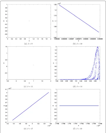
On the basis of Theorem2.1, we know that system (1.5) has three boundary nonnegative equilibrium pointsE0(0, 0),E1(1, 0) andEm(m, 0). ForE1(1, 0), its two eigenvalues areλ1=

m< 1 andλ2=exp(β–γ).

Varyβin the range 5≤β≤20, and ﬁxm= 0.1,α= 1,γ = 10. The bifurcation diagram is plotted in Fig.1(a)–(d). We see that the equilibrium pointE1(1, 0) is stable for 5 <β< 12, and loses its stability at the fold bifurcation parameter valueβ= 12. Moreover, a chaotic set emerges with the increasing ofβ. But, from Fig.1(b) and (d), we know that whenβ increases to some ﬁxed value the prey (predator) becomes extinct.

The maximum Lyapunov exponents corresponding to Fig.1are calculated and plotted in Fig.2.

The phase portraits are plotted in Fig.3. From Fig.3(a)–(f ), we can see the predator is ex-tinct. Predator and prey are extinct from Fig.3(f ). Figures1–3illustrate that Theorem3.1

is correct.

5 Result and discussion

(13)

Figure 1The dynamics ofxandy

Figure 2Maximum Lyapunov exponents corresponding to Fig.1

predator, the fold bifurcation will occur at this system. Some more interesting dynamical properties, such as chaos, are also obtained by a numerical simulation, which shows that the system is worthy of further theoretical research.

(14)

Figure 3Phase portrait of the system (1.5) versusβ

properties of this system may be highly sensitive to the living environment. It deserves fur-ther consideration as regards the Allee eﬀect and the interaction of a ratio-related predator on the living environment of the populations.

(15)

contin-uous model. This further implies that it is meaningful to study the discretization of the continuous model.

Acknowledgements

The authors sincerely thank the reviewers for their valuable suggestions and useful comments that have led to the present improved version.

Funding

This work of the ﬁrst author is supported by Natural Science Foundation of China under grant No. 11701513 and No. 11426203. This work of the second author is supported by Natural Science Foundation of China under grant No. 61473340 and Natural Science Foundation of Zhejiang University of Science and Technology under grant No. F701108G14.

Competing interests

The authors declare that they have no competing interests.

Authors’ contributions

All authors contributed equally and signiﬁcantly in writing this paper. All authors have read and approved of the ﬁnal manuscript.

Publisher’s Note

Springer Nature remains neutral with regard to jurisdictional claims in published maps and institutional aﬃliations. Received: 11 April 2018 Accepted: 27 August 2018

References

1. Aguirre, P., Flores, D., González-Olivares, E.: Bifurcations and global dynamics in a predator–prey model with a strong Allee eﬀect on the prey, and a ratio-dependent functional response. Nonlinear Anal., Real World Appl.16, 235–249 (2014)

2. Aguirre, P., González-Olivares, E., Torres, S.: Stochastic predator–prey model with Allee eﬀect. Nonlinear Anal., Real World Appl.14(1), 768–779 (2013).https://doi.org/10.1016/j.nonrwa.2012.07.032

3. Arditi, R., Saiah, H.: Empirical evidence of the role of heterogeneity in ratio-dependent consumption. Ecology73, 1544–1551 (1992)

4. Arditi, R., Ginzburg, L.: Coupling in predator–prey dynamics: ratio-dependance. J. Theor. Biol.139, 311–326 (1989) 5. Berec, L., Angulo, E., Counchamp, F.: Multiple Allee eﬀects and population management. Ecol. Model.22, 185–191

(2006)

6. Chen, B., Chen, J.: Bifurcation and chaotic behavior of a discrete singular biogical economic system. Appl. Math. Comput.219(5), 2371–2386 (2012)

7. Chicone, C.: In: Ordinary Diﬀerential Equations with Applications, 2nd edn. Texts in Applied Mathematics, vol. 34. Springer, Berlin (2006)

8. Courchamp, F., Berec, L., Gascoigne, J.: Allee Eﬀects in Ecology and Conservation. Oxford University Press, London (2008)

9. Gause, G.: The Struggle for Existence. Williams & Wilkins, Baltimore (1934)

10. Gascoigne, J., Lipcius, R.: Allee eﬀects in marine systems. Mar. Ecol. Prog. Ser.269, 49–59 (2004)

11. Haque, M.: Ratio-dependent predator–prey models of interacting populations. Bull. Math. Biol.71, 430–452 (2009) 12. Han, W., Liu, M.: Stability and bifurcation analysis for a discrete-time model of Lotka–Volterra type with delay. Appl.

Math. Comput.217(12), 5449–5457 (2011)

13. He, Z., Lai, X.: Bifurcation and chaotic behavior of a discrete-time predator–prey system. Nonlinear Anal., Real World Appl.12(1), 403–417 (2011)

14. Hu, Z., Teng, Z., Zhang, L.: Stability and bifurcation analysis of a discrete predator–prey model with nonmonotonic functional response. Nonlinear Anal., Real World Appl.12(4), 2356–2377 (2011)

15. Jana, D.: Chaotic dynamics of a discrete predator–prey system with prey refuge. Appl. Math. Model.224, 848–865 (2013)

16. Ghaziani, R.K., Govaerts, W., Sonck, C.: Resonance and bifurcation in a discrete-time predator–prey system with Holling functional response. Nonlinear Anal., Real World Appl.13(3), 1451–1465 (2012).

https://doi.org/10.1016/j.nonrwa.2011.11.009

17. Kuzenetsov, Y.: Elements of Applied Bifurcation Theory, 3rd edn. Applied Mathematical Sciences, vol. 112. Springer, New York (2004).https://doi.org/10.1007/978-1-4757-3978-7

18. Lu, H., Wang, W.: Dynamics of a delayed discrete semi-ratio-dependent predator–prey system with Holling type IV functional response. Adv. Diﬀer. Equ.2011, 7 (2011)

19. Li, X.: Bifurcation analysis of a predator–prey system with sex-structure and sexual favoritism. Adv. Diﬀer. Equ.2013, 219 (2013).https://doi.org/10.1186/1687-1847-2013-219

20. Misra, O., Sinha, P., Singh, C.: Stability and bifurcation analysis of a prey–predator model with age based predation. Appl. Math. Model.37(9), 6519–6529 (2013).https://doi.org/10.1016/j.apm.2013.01.036

21. Robinson, C.: Dynamical Systems: Stability, Symbolic Dynamics, and Chaos. CRC Press, London (1995)

22. Ruan, S., Xiao, D.: Global analysis in a predator–prey system with nonmononotonic functional response. SIAM J. Appl. Math.61(4), 1445–1472 (2001)

(16)

24. Wang, C., Li, X.: Further investigations into the stability and bifurcation of a discrete predator–prey model. J. Math. Anal. Appl.422, 920–939 (2015)

25. Xiao, D., Ruan, S.: Global dynamics of ratio-dependent predator–prey system. J. Math. Biol.43(3), 268–290 (2001).