R E S E A R C H
Open Access
Optimizing distance, transmit power, and
allocation time for reliable multi-hop relay system
Pham Thanh Hiep
*, Fumie Ono and Ryuji Kohno
Abstract
In multi-hop relay systems, the end-to-end channel capacity is restricted by bottleneck node. In order to prevent some relay nodes from being the bottleneck of system and to guarantee the end-to-end channel capacity, the method of optimizing transmit power, distance and allocation time is proposed in this article. We show that the optimizing distance has more end-to-end channel capacity than the optimizing transmit power in case that both the distance and the transmit power are changeable. However, the optimizing transmit power can let the system reach high end-to-end channel capacity when the relay nodes have to shift from the desired location. We also propose the Markov Chain Monte Carlo method to optimize all transmit power, distance and allocation time simultaneously. The optimizing all transmit power, distance and allocation time is the most effective and achieves the highest channel capacity. Based on the average signal-to-noise-ratio, the average channel capacity is evaluated in this article.
1 Introduction
In the future, it is believed that the MIMO service area will become popular. Therefore, a MIMO relay system is considered. However, in a relay system with one relay, when the number of relay antenna elements is less than the number of transmitter and receiver antenna elements, the capacity of MIMO relay system is lower than that of the original MIMO system. In addition, when the number of relay antenna elements is equal to or more than the number of the transmitter and receiver antenna elements, a MIMO relay system can provide the same average capa-city as an original MIMO system. In other words, although the number of relay antenna elements is larger than the transmitter and receiver antenna elements, the capacity of MIMO relay system cannot exceed the channel capacity of original MIMO system [1-3].
Therefore, a system with multi relays called multi-hop relay system was proposed and have been discussed in several literatures. The Gaussian MIMO relay channel with fixed channel condition has derived upper bounds and lower bounds that can be obtained numerically by convex programming [4-6]. Moreover, the capacity of a particular large Gaussian relay network is determined by the limit as the number of relays tends to infinity [7]. In
addition, a multi-hop relay network with multi antenna terminals in a quasi-static slow fading environment also has been considered [8]. However, these researches assumed the signal-to-noise-ratio (SNR) at receiver(s) is fixed, the distance between the transceivers and the transmit power of transmitter(s) are not considered.
In multi-hop MIMO relay systems, when the distance between the base station (Tx) and the final receiver (Rx) is fixed, the distance between the Tx to a relay node (RS), an RS to an RS, an RS to the Rx called the distances between transceivers, is shorten. Consequently, the SNR and the channel capacity are increased. However, accord-ing to the number of the relay nodes, the location and the transmit power of each relay node; the channel capa-city of each relay node is changed. In addition, the end-to-end channel capacity is limited by bottleneck node. Therefore, to obtain the upper bound of end-to-end channel capacity, the location of each relay node meaning the distance between the transceivers and the transmit power of each relay node need to be optimized. We have analyzed performance of multi-hop MIMO relay system with amplify-and-forward (AF) [9]. The distance between the transceivers is optimized when the transmit power of each relay node is assumed to be equal. However, the location of the relay nodes is not always changeable. Consequently, in order to obtain a certain value of end-to-end channel capacity, the distance and the transmit
* Correspondence: [email protected]
Division of Physics Electrical and Computer Engineering, Graduate School of Engineering, Yokohama National University, Yokohama, 240-8501, Japan
power need to be optimized. In this article, the distance and the transmit power are optimized separately or simultaneously to guarantee the end-to-end channel capacity in decode-and-forward scheme multi-hop relay systems. In addition, allocation time is optimized to guar-antee and/or to obtain the higher end-to-end channel capacity. Moreover, the channel capacity that is men-tioned in this article is average channel capacity. The rest of the article is as follows. After the introduction of the system model in Section 2, we propose the optimizing method of transmit power and distance in Section 3 and the optimizing method of allocation time in Section 4. The optimizing of all transmit power, distance and allo-cation time simultaneously is described in Section 5. Finally, Section 6 concludes the article.
2 Multi-hop MIMO relay system 2.1 System model
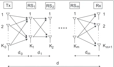
Figure 1 shows mrelays intervened multi-hop MIMO relay system. Here,Ki(i= 0, . . . ,m+ 1) denotes the
num-ber of the antenna elements at the Tx, the Rx and each relay node. di (i = 0, . . . ,m) represents the distance
between the transceivers. The distance between the Tx and the Rx is fixed asd. The signal is transmitted from the Tx to theRS1. At theRS1, the signal is decoded, encoded
and transmitted to theRS2. Similarly, the signal is
trans-mitted over and over until the signal reaches to the final
receiver. We assumed the transmit power of theTx (ETx) and the total transmit powers of relay node (ERS) are fixed regardless of the number of the relay nodes and the num-ber of antenna elements at each relay. The transmit power of each relay node is denoted byEi. Moreover, the trans-mit power of each relay is equally divided into each antenna element. On the other hand, as described in Sec-tion 1, if the number of antenna elements at one relay is smaller than the other, this relay will be a bottleneck of the system and the end-to-end channel capacity will be restricted by this relay. Since in this article we consider the distance, transmit power and allocation time, the num-ber of antenna elements at each relay is assumed to be the same as that of the Txand theRx and denoted by M. Moreover, we assume that the time-division-multiple-access (TDMA) algorithm is applied to control the trans-mission of each relay node. The allocation time ofRSiis
denoted asti.
LetHii+1denotes aKi+1×Kichannel matrix between the RSiand theRSi+1. Since the path loss is taken into
consid-eration, Hii+1is the composite matrix. We modelHii+1as
Hii+1=
lii+1Hwii+1, i = 0,. . ., m, (1)
whereHwii+1is a matrix with independent and
identi-cally distributed (i.i.d.), zero mean, unit variance, circu-larly symmetric complex Gaussian entries, and lii+1
Tx
RS
Rx
1
2
K
1
2
K
1
K
1
K
1
1
K
2
RS
2
RS
m
m
1
d
0
d
1
d
m
d
0
m+1
represents the path loss between theRSi and theRSi+1.
The path loss is described in detail in the following section.
2.2 Path loss
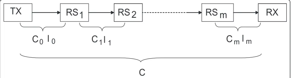
Since there are a lot of obstacles, such as huge buildings, in propagation environment, the path loss is necessary to consider being attenuated by the reflection. The power of the signal is reduced when the reflection occurs. An amount of the reduction by one time of reflection is called reflection factor. It is natural that the reflection factor is changed according to the matter of the obstacles, the angle of reflections and so on. However, in this article, the reflection factor of all reflections is assumed to be the same and denoted bya. The path loss between the trans-ceivers is described in Figure 2. The path loss in this case is expressed as [10]
li=
whererefiis the number of reflection while a signal is
transmitted betweenRSiandRSi+1. In addition, in order to
obtain the number of reflection, the propagation environ-ment coefficientWiis defined as the average distance from
a reflection point to the next reflection point. In other words, it is the average of line-of-sight (LOS) distance betweenRSiandRSi+1. Therefore, the number of reflection
between the transceivers can be expressed as refi= Wdii.
Consequently, the path loss in (2) can be rewritten as
li=
Let the channel capacity between the RSiand theRSi+1
isCi, andCdenotes the end-to-end channel capacity of
the multi-hop MIMO relay system (Figure 2).
The transmission in multi-hop relay system is assumed to be controlled accurately. There-fore, when the signalSi-1 is transmitted from theRSi-1, the received
signal at theRSiis expressed as cite9, Si=Hi−1i
Pi−1Si−1+ni. (4)
Here, Pi= diag(pi1, pi2,. . .,piKi) is the transmit power
matrix and is assumed to be subject to a constraint
Tr(Pi)= ETx(i= 0),
Ei (i= 0),
where Tr(·) and pij denote the trace and transmit
power ofjthantenna element of RSi, respectively.niis
the noise vector with i.i.d., zero mean, s2variance. The transmit power of every antenna in the same relay node was assumed to be equal.
pi1=pi2=· · ·=piKi=
Ei
M.
Moreover, the channel capacity is represented as follows.
Ci= log2
capacity of each relay node is independent from each other, the end-to-end channel capacity is equal to chan-nel capacity of bottleneck relay node.
C= min(t0C0, t1C1, . . ., tmCm). (6)
3 Optimizing transmit power and distance
In order to explain the optimizing of the distance and transmit power clearly, the allocation time of each relay node is assumed to be the same, ti= m1+1. In addition,
Hwii + 1H
H
wii + 1 (i= 0, . . . ,m) is independent from the
dis-tance and the transmit power. Consequently, the SNR can be examined instead of a channel capacity. Hence, in order to avoid that some nodes become the bottleneck
RS
1
RS
2
RS
m
RX
TX
l
0
C
1
l
1
C
m
l
m
C
0
C
and to obtain high channel capacity, the channel capacity of each node should be equal. Consequently, the received SNR of each node is necessary to be equal.
SNRi=SNRj, fori=j, i,j= 0,. . .,m, (7)
3.1 Optimizing transmit power 3.1.1 Optimization method
When the location of the relay nodes is not changeable, the transmit power of each relay node should be opti-mized to increase the channel capacity of bottleneck relay node. Consequently, the necessary transmit power can be obtained from (7).
Eili
Mσ2 = Ejlj
Mσ2, fori=j, i,j= 1,. . .,m. (8)
Note that total transmit power of relay node is fixed.
m
By substituting eachEito (9), it can be rewritten as
E1+
Consequently, the necessary transmit power ofRS1 is
obtained.
Similarly, the transmit power of each relay node is obtained by,
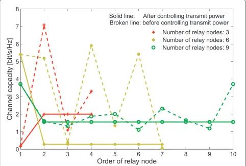
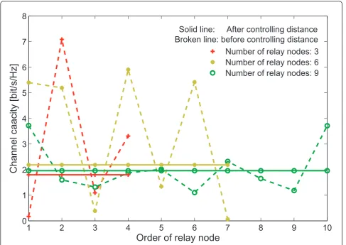
3.1.2 Numerical evaluation of optimizing transmit power
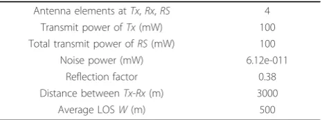
The system parameters summarized in Table 1 are used as an example for evaluating the optimizing method men-tioned above. Let the distance between the transceivers be random. The channel capacity, in case the number of the
relay nodes are 3, 6, 9, are described in Figure 3, here the average propagation environment coefficient W,
W= m
i=0Wi
m+1 , meaning the average of LOS distance
between theTxandRx, is set as 500 m.
As shown in Figure 3, in case the number of the relay nodes is 9, the channel capacity of bottleneck node is improved and the end-to-end channel capacity is increased. However, since the transmit power ofTxis assumed to be constant, the channel capacity ofRS1is fixed. Therefore
RS1becomes a bottleneck node ifd0is large, such as the
number of the relay nodes is 3. In this case, the end-to-end channel capacity can not be improved. Moreover, SNR is increased by transmit power to the 1st power and decreased by distance to the 2nd power. Hence, in order to increase the channel capacity, the huge transmit power needs to be provided when the distance is large. Under the assumption that total transmit power of relay node is fixed; the channel capacity is not considerably improved. It is the reason why the end-to-end channel capacity of the system with 6 relay nodes is low.
3.2 Optimizing distance between transceivers 3.2.1 Optimization method
Since the optimizing of transmit power remains some drawbacks as mentioned above, the distance between the transceivers needs to be considered. In order to ana-lyze the distance more easily, the transmit power of each relay node is assumed to be equal. Therefore, the channel capacity only depends on the distance.
By solving (7), the optimized distance becomes as follows.
li=lj, fori=j, i,j= 1,. . .,m,
ETxl0= ERS
m li.
Firstly, at scheme 1, we assume that all channel mod-els between the transceivers are the same (W ). There-fore, by substituting the path loss of (3) in (7), this equation becomes,
Table 1 Numerical parameters
Antenna elements atTx,Rx,RS 4 Transmit power ofTx(mW) 100 Total transmit power ofRS(mW) 100
Noise power (mW) 6.12e-011
Reflection factor 0.38
Distance betweenTx-Rx(m) 3000
Let
g(di)=a(m+1)dWi−d.
The Taylor expansion is approximate tog(di), and (14)
can be expressed as
b4d4i +b3d3i +b2d2i +b1di+b0= 0, (15)
(15) is rewritten as
x4+px2+qx+r= 0, (16)
The functionyis added to this equation.
x4+p+yx2+r=yx2−qx. (17)
Moreover, we can describe as
x4+px2+qx+r=x2+c1x+c0 x2+d1x+d0
Order of relay node
Channel capacity [bit/s/Hz]
Number of relay nodes: 3
Number of relay nodes: 6
Number of relay nodes: 9
Solid line: After controlling transmit power
Broken line: before controlling transmit power
Therefore,
c1+d1= 0, c0+d0+c1d1=p, c1d0+c0d1=q,c0d0=r.
From these equations, the resolvent cubic equation can be obtained.
c21c21+p2−q2= 4c21r. (20)
Let c2
1=y, the resolvent cubic equation can be
rewrit-ten as
yy+p2−q2= 4yr. (21)
From this equation, functionyis obtained.
y= 1
Additionally, by applying the resolvent cubic equation to (18), we have
Consequently, the functionxcan be obtained.
x1,2=
As a result, the optimized di can be obtained by di=x− 4bb34 with the condition thatdiis a real number
within (0,d). For the system parameter described in the
next section, only
In analyzing the performance of the system that has all channel models between the transceivers which are differ-ent, (Wi) is similar. The system in this case is indicated for
scheme 2. The Taylor expansion is approximately used for a term a−2di
Wi . Then, the partial differential equation with
respect to eachdiis obtained, and eachdican be obtained
similarly to be mentioned above. However, in this case, we
have made the Taylor expansion, solving partial differen-tialm+ 1 times to obtain eachdi.
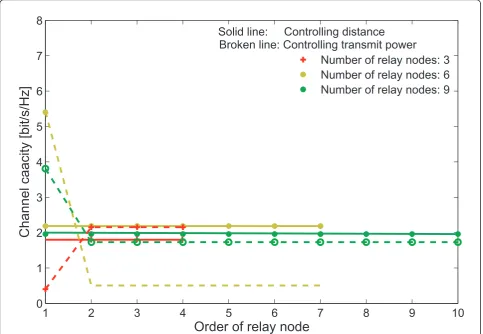
3.2.2 Numerical evaluation of optimizing distance
The system model is the same as mentioned above, and the system parameters are summarized in Table 1. Fig-ure 4 shows the end-to-end channel capacity responded to each number of the relay nodes, i.e., 3, 6, 9.
By contrast to the optimizing of the transmit power, the optimizing of the distance can change the channel capacity ofRS1 and improve the channel capacity of all
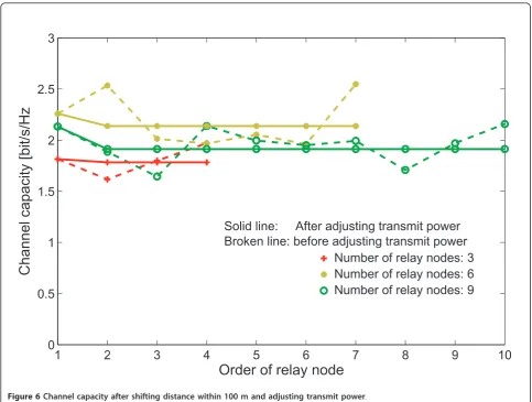
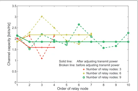
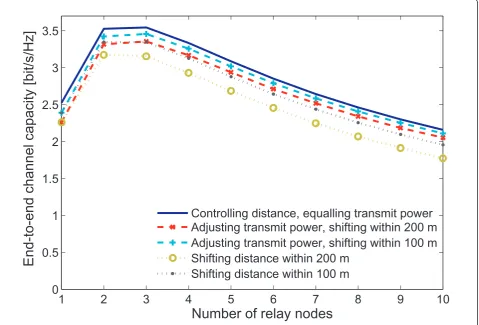
bottleneck nodes. The comparison in channel capacity of optimizing the distance and optimizing the transmit power is shown in Figure 5. It is clear that in the case of optimizing the distance, the channel capacity of all relay nodes is the same and relatively higher than the end-to-end channel capacity in the case of optimizing the transmit power. The optimizing of the distance is effective; however, the relay node can not always be set at the desired location. For example, the desired location is on roads, in rivers, and so on. Thus, the relay node needs to be shifted in the front or the rear of the desired location. As a result, the channel capacity is decreased. In order to remain high channel capacity, the transmit power is adjusted after shifting distance by method of optimizing transmit power mentioned above. Figures 6 and 7 show the end-to-end channel capacity before and after adjusting the transmit power. In this scenario, the channel capacity of all relay nodes after adjusting the transmit power is almost the same, and achieves the end-to-end channel capacity of the system without shifting the location of the relay nodes. The optimizing of the transmit power in this scenario is much more effective.
In order to compare the end-to-end channel capacity when the number of the relay nodes is changed, the average end-to-end channel capacity from 1, 000×of calculation is shown in Figure 8. The end-to-end chan-nel capacity is increased when the number of the relay nodes is small. Moreover, when the number of the relay nodes exceeds a certain value, the end-to-end channel capacity is decreased. The reason is that the SNR increases when the number of the relay nodes increases, however the allocation time of each relay node reduces rapidly. Therefore, although the SNR is high, the end-to-end channel capacity is decreased. As a result, there is the optimum number of the relay nodes for maximum end-to-end channel capacity.
is approximate to the end-to-end channel capacity of the system without shifting the location of the relay nodes.
4 Optimizing allocation time
4.1 Optimization method of allocation time
Similar to transmit power and distance, in order to guarantee the end-to-end channel capacity, the alloca-tion time of each relay needs to be optimized. To explain the optimizing of the allocation time, we assume all distance and transmit power to be fixed. When every relay transmits the signal in its allocation time, the end-to-end channel capacity is as follows.
C= min(tiCi), (i= 0,. . .,m). (26)
The practicable channel capacity of the system is guaranteed when
tiCi=tjCj, (i=j).
As a result,
ti t0
= C0
Ci , m
i=1ti t0
=C0
m
j=1 1
Cj .
(27)
Therefore, the optimized allocation time is expressed as
t0=
1 1 +C0
m j=1
1
Cj
, (28)
ti=
j=i+1
Cj
m j=1
k=j
Ck
, (i= 1,. . .,m). (29)
Consequently, the channel capacity of each relay node is the same and the end-to-end channel capacity is expressed as follows.
1
2
3
4
5
6
7
8
9
10
0
1
2
3
4
5
6
7
8
Order of relay node
Channel caacity [bit/s/Hz]
Number of relay nodes: 3
Number of relay nodes: 6
Number of relay nodes: 9
Solid line: After controlling distance
Broken line: before controlling distance
C= m1 i=0C1i
. (30)
From (30), we have
C≥ m 1
i=0min(1Ci)
= 1
m+ 1min(Ci). (31)
It means that the end-to-end channel capacity of the system after optimizing allocation time is higher than that of the system with equal allocation time.
4.2 Numerical evaluation of optimizing allocation time In this section, the optimizing of the distance, the trans-mit power and the allocation time by mathematical method at scheme 1 is compared. The channel model is the same as mentioned above. Figure 9 shows the chan-nel capacity of each relay node in case the number of the relay nodes are 3 and 9. In the case of 3 relay nodes, the difference of channel capacity before and after optimizing the allocation time is small. It can be
explained that if there is a relay node that has the chan-nel capacity much smaller than that of another, the end-to-end channel capacity before and after optimizing allo-cation time is restricted by this relay node. In the case of optimizing allocation time, let’s assume that the chan-nel capacity of RSk is the lowest (Ck ≪ Ci, i ≠k,). It means C1
k
1
Ci. Consequently, the end-to-end channel capacity in (30) can be changed as follows.
C≈ 11
Ck
=Ck. (32)
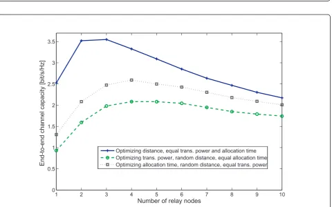
However, as mentioned in the previous section, the end-to-end channel capacity after optimizing allocation time is higher than that before the optimizing. Addition-ally, the end-to-end channel capacity of optimizing allo-cation time is lower than that of optimizing distance, but higher than that of optimizing transmit power (in the case of 9 relay nodes in Figure 9). We can confirm the relation between optimization results to Figure 10. Figure 10 shows the average from 1, 000 × calculation
1
2
3
4
5
6
7
8
9
10
0
1
2
3
4
5
6
7
8
Order of relay node
Channel caacity [bit/s/Hz]
Number of relay nodes: 3
Number of relay nodes: 6
Number of relay nodes: 9
Solid line: Controlling distance
Broken line: Controlling transmit power
of the end-to-end channel capacity when the number of the relay nodes is changed from 1 to 10.
5 Optimized transmit power, distance, and allocation time simultaneously
Till now, we explained the method of optimizing trans-mit power, distance and allocation time separately in Sections 3 and 4. Each method is effective. However, the optimizing of the transmit power, the distance and the allocation time simultaneously is expected to achieve higher channel capacity than optimizing each one separately.
5.1 Mathematical method
In order to optimize the transmit power, the distance and the allocation time, firstly let’s fix the distance, equalize the allocation time and optimize the transmit power. Therefore, the optimization method and the result in Section 3 can be applied and (7) can be rewrit-ten by
ETxl0= ERS m
i=11li
. (33)
To solve this equation, each path loss should be expressed by Taylor expansion. It is relatively complex, especially at scheme 2. Consequently, in order to opti-mize the distance, the transmit power and the allocation time more easily in any channel model, the Markov Chain Monte Carlo (MCMC) method is proposed in the following section. Moreover, from (13), theSNRican be expressed as follows.
SNRi= Eili
Mσ2,
= ERS
Mσ2 1
m
i=11li ,
≤ ERS
Mσ2
m
m
i=1 4πdi λa
di
Wi
2.
(34)
1
2
3
4
5
6
7
8
9
10
0
0.5
1
1.5
2
2.5
3
Order of relay node
Channel capacity [bit/s/Hz
Number of relay nodes: 3
Number of relay nodes: 6
Number of relay nodes: 9
Broken line: before adjusting transmit power
Solid line: After adjusting transmit power
Thus, whenWianddi,i= 1, . . . ,mare equal, respec-tively (the optimum distance of scheme 1),SNRibecomes
maximum. In this case, the equal allocation time is also the optimum solution. In other words, the optimized dis-tance, transmit power and allocation time at scheme 1 is one of the optimal solutions for maximal end-to-end channel capacity of any channel model. Consequently, the optimizing of the distance, the transmit power and the allocation time lets the end-to-end channel capacity reach to this maximum.
5.2 Markov chain Monte Carlo method
The MCMC method is constructed to find the optimal state of transmit power, distance and allocation time that has the end-to-end channel capacity close to the maximal channel capacity. The algorithm is explained as follows.
Calculate W= (m1+1)mi=0(Wi) and maximal channel capacity Cmax (optimize transmit power, distance and
allocation time at scheme 1).
Step 1: Createdi,Eiand tirandomly. Subject to
m
i=0
(di) =d,
m
i=1
(Ei) =ERS,
m
i=0
(ti) = 1.
Step 2: Calculate all channel capacitiesCi, and soften
them from high to low. Adjust the distance, the transmit power and the allocation time to make all channel capa-city to be almost the same.
di=di+(dm−i−di)rand1, dm−i=dm−i−(dm−i−di)rand1, (35)
ti=ti−(ti−tm−i)rand2, tm−i=tm−i+ (ti− tm−i)rand2, (36)
Ei=Ei−(Ei−Em−i)rand3, Em−i=Em−i+(Ei−Em−i)rand3,
except ETX
, (37)
here, rand1, rand2, rand3 are random value within (0,1). Iterate step 2 until standard deviation of all chan-nel capacities is smaller than sigma (s).
Step 3: If end-to-end channel capacity of scheme 2 is
close to maximal channel capacity Cmax−C
Cmax ≤α
, the
algorithm is finished. Otherwise, return to step 1. Compare to the mathematical method, MCMC algo-rithm is easier to optimize the distance, the transmit power and the allocation time simultaneously at any channel model. However, the MCMC algorithm requests running in the computer and the convergence of this algorithm should be discussed. The convergence is dependent on sand a, if s is not tight enough, the
1
2
3
4
5
6
7
8
9
10
0
0.5
1
1.5
2
2.5
3
3.5
Order of relay node
Channel capacity [bit/s/Hz]
Number of relay nodes: 3
Number of relay nodes: 6
Number of relay nodes: 9
Broken line: before adjusting transmit power
Solid line: After adjusting transmit power
algorithm doesn’t converge. On the other hand, if sis too tight, the algorithm takes a long time for conver-gence. Hence, for each a, the suitable sneeds to be considered.
Let’s denote the average of all channel capacities to beC¯. When the end-to-end channel capacity (C= min(Ci)) is approximate to the maximal channel capacity (Cmax), we
have C¯ ≈ Cmaxand|max(Ci)− ¯C| ≈ |min(Ci)− ¯C|. Thus,scan be described by
σ2= 1
Cmax changes when the number of the relay nodes
changes. s is changed for each number of the relay nodes anda. Figure 11 shows the end-to-end channel capacity in case s is changed, i.e., 1%, 5%, and 10%. Here, let Wi be random within (0, 1000) and satisfy
1
m+1
m
i=0Wi= 500. According to a, the end-to-end channel capacity of MCMC method is different. How-ever, with small alpha, MCMC method optimizes the transmit power, the distance, the allocation time simul-taneously and achieves the maximal channel capacity in any channel model.
6 Conclusion
In this article, we examined the performance of multi-hop relay systems with decode-and-forward method. The optimizing of the transmit power, the distance and the allocation time is effective in preventing some relay nodes from becoming the bottleneck of the system and in guaranteeing the end-to-end channel capacity. How-ever, the optimizing of the distance is the most effective and the optimizing of the transmit power is the least effective. The optimizing of the transmit power is effec-tive when the location of the relay nodes is shifted within a short range from the desired location. The
1
2
3
4
5
6
7
8
9
10
Number of relay nodes
End-to-end channel capacity [bit/s/Hz]
Controlling distance, equalling transmit power
Adjusting transmit power, shifting within 200 m
Adjusting transmit power, shifting within 100 m
Shifting distance within 200 m
Shifting distance within 100 m
1 2 3 4 5 6 7 8 9 10 0
1 2 3 4 5 6
Order of relay node
Channel capacity [bit/s/Hz]
Before optimize (random distance, equal trans. power) Optimizing allocation time
Optimizing trans. power Optimizing distance Broken line: 3 relay nodes Solid line: 9 relay nodes
Figure 9Channel capacity of optimizing the transmit power, the distance and the allocation time when the number of relay nodes are 3 and 9.
1 2 3 4 5 6 7 8 9 10
0 0.5 1 1.5 2 2.5 3 3.5
Number of relay nodes
End-to-end channel capacity [bit/s/Hz]
Optimizing distance, equal trans. power and allocation time Optimizing trans. power, random distance, equal allocation time Optimizing allocation time, random distance, equal trans. power
MCMC algorithm was proposed to optimize all transmit power, distance and allocation time simultaneously. MCMC method can achieve the maximal channel capacity.
In this article, in order to simplify the analysis, we have analyzed the system under Gaussian channel model. However, the performance of this system needs to be analyzed under the channel model which is close to the practice. Additionally, in order to apply the opti-mization method to any channel model, more general path loss functions needs to be considered. We consid-ered the transmit power, the distance and the allocation time to guarantee the end-to-end channel capacity. The other method, such as the changing of modulation and/ or coding is left for future studies.
Competing interests
The authors declare that they have no competing interests.
Received: 13 October 2011 Accepted: 30 April 2012 Published: 30 April 2012
References
1. M Tsuruta, Y Karasawa, Multi-Keyhole model for MIMO repeater system evaluation. IEICE Trans Commun.J89-B(9), 1746–1754 (2006)
2. D Chizhik, GJ Foschini, MJ Gans, RA Valenzuela, Keyholes, correlations, and capacities of multi-element transmit and receive antennas. IEEE Trans Wirel Commun.1(2), 361–368 (2002). doi:10.1109/7693.994830
3. G Levin, S Loyka, On the outage capacity distribution of correlated keyhole MIMO channels. IEEE Trans Inf Threory.54(7), 3232–3245 (2010)
4. B Wang, J Zhang, A host-Madsen, On the capacity of MIMO relay channel. IEEE Trans Inf Theory.51(1), 29–43 (2005)
5. DS Shiu, GJ Foschini, MJ Gans, JM Kahn, Fading correlation and its effect on the capacity of multi-element antenna systems. IEEE Trans Commun.48(3), 502–513 (2000). doi:10.1109/26.837052
6. D Gesbert, H Bolcskei, DA Gore, AJ Paulraj, MIMO wireless channel: capacity and performance prediction. Proc GLOBECOM.2, 1083–1088 (2000) 7. M Gastpar, M Vetterli, On the capacity of large Gaussian relay networks. IEEE
Trans Inf Theory.51(3), 765–779 (2005). doi:10.1109/TIT.2004.842566 8. D Giindiiz, MA Khojastepour, A Goldsmith, H Vincent Poor, Multi-hop MIMO
relay networks: diversity-multiplexing trade off analysis. IEEE Trans Wirel Commun.9(5), 1738–1747 (2010)
9. PT Hiep, R Kohno, Optimizing position of repeaters in distributed MIMO repeater system for large capacity. IEICE Trans Commun.E93-B(12), 3616–3623 (2010). doi:10.1587/transcom.E93.B.3616
10. N Kita, W Yamada, A Sato, Path loss prediction model for the over-rooftop propagation environment of microwave band in suburban areas. IEICE Trans Commun.J89-B(2), 115–125 (2006). (in Japanese)
doi:10.1186/1687-1499-2012-153
Cite this article as:Hiepet al.:Optimizing distance, transmit power, and allocation time for reliable multi-hop relay system.EURASIP Journal on Wireless Communications and Networking20122012:153.
1 2 3 4 5 6 7 8 9 10
0 0.5 1 1.5 2 2.5 3 3.5
Number of relay nodes
End-to-end channel capacity [bits/s/Hz]
Solid line: Mathematical method for scheme 1
alpha = 1% alpha = 5% alpha = 10%
Broken line: MCMC method for scheme 2