R E S E A R C H
Open Access
Multicarrier code for the next-generation GPS
Donglin Wang
1,2*, Michel Fattouche
1and Fadhel M Ghannouchi
1Abstract
This article investigates multicarrier (MC) transmission for next-generation global positioning system (GPS) instead of current spread spectrum signals. A MC code is proposed in this article as an alternative to the coarse/acquisition (C/A) code in GPS. The entire GPS bandwidth for the C/A code is divided into 1,024 subcarrier slots. As per our proposed arrangement, each satellite vehicle (SV) takes up only 42 uniformly spaced and non-overlapping subcarrier slots while approximately occupying the same bandwidth as the C/A code in GPS. In this way, the proposed MC code is proved to attain a 4.73 dB SNR gain compared to the GPS C/A code in terms of Cramer-Rao lower bound for range estimation, which could evidently enhance the GPS receiver’s sensitivity. Together with the feature of robustness against multipath effect, the proposed MC code is helpful for urban, tunnel, even indoor and underground positioning. The transmission and reception of the propose MC code is also described, where the range estimation process is explained. Furthermore, the proposed MC code is shown to be robust against narrow band interference. Moreover, the probability of collision between SVs due to Doppler shifts is theoretically analyzed, where the probability of successful positioning is evaluated. Simulation Results show a consistency with our proposed theory.
Keywords:multicarrier code, GPS C/A code, SNR Gain, doppler effect, NBI, probability of collision
1 Introduction
Global navigation satellite system (GNSS) such as the current global positioning system (GPS) or the future European Galileo system can provide a worldwide accu-rate positioning under an outdoor good environmental conditions [1]. However, GNSS based positioning is not reliable in urban, tunnel, underbridge, indoor or under-ground environments due to the dense multipath effect as well as non-line-of-sight (NLOS) signal energy attenuation [1]. As it is known, multicarrier (MC) signals, e.g. orthogonal frequency division multiplexing (OFDM) signals [2,3], are robust against the multipath effect [4-8]. Furthermore, they have a more efficient spectrum usage compared to the current golden codes [9,10], which thus leads to a SNR gain for range estimation. Therefore, the MC signal is being considered for investigation of the possiblity of its application in next-generation GNSS.
For the best of authors’knowledge, the use of a MC signal as a code of next-generation GNSS is investigated by both [1,11]. Zanier and Luise [11] discussed about the funamental issues in time-delay estimation of MC
signals with applications to next-generation GNSS. This article used a filter bank MC modulation, where the MC modulation has the same power spectral density (PSD) of the current golden code so that they have the same ranging performance. Furthermore, Zanier and Luise [11] derived the fundamental performance of the filter bank MC modulation using Cramer-Rao lower bound (CRLB). Dai et al. [1] tried to propose the OFDM/MC based scheme for the next-generation GNSS. However, authors basically discussed the OFDM communication and the performance of time-of-arrival (TOA) estima-tion, which are too far from an available GNSS scheme. As we know, it is impossible for all SVs to use the same OFDM signal when the frequency collision between SVs will occur and the data reception will fail without ques-tion. Dai et al. [1] only gave a general discussion but did not provide the specific probing signal for each satellite vehicle (SV). Also, it did not compare the OFDM signal with the current GNSS code in terms of ranging and/or positioning accuracy. Furthermore, it did not analyze the scheme’s feasibility as an option of the next-genera-tion GNSS.
Differently from the previous literature, this article investigates the possiblity of a unfiltered non-data-bear-ing MC modulation applied in the next-generation
* Correspondence: [email protected]
1ECE Department, University of Calgary, Calgary, AB, T2N 1N4, Canada
Full list of author information is available at the end of the article
GNSS instead of the current golden code. Specifically, a MC code is proposed as an alternative to the coarse/ acquisition (C/A) code for the next-generation GPS. As we all know, GPS transmits three binary codes for target navigation: the pseudo-random noise (PN) based C/A code with 1.023 MHz, the PN-based precise (P) code with 10.23 MHz and the navigation message with 50 bps [12-15]. Among them, the C/A code is for civilian use but performs poor under the dense multipath effect, e.g. positioning in a downtown environment, weak signal detection such as indoor or underground positioning and narrow band interference (NBI).aConsequently, the MC modulation is proposed as a next-generation alter-native to the C/A code in order to improve the position-ing performance against multipath, weak signal and NBI. Even though the multipath management in the commu-nication area is different from that in the GNSS area, the topic of the multipath management is not addressed in the article.
In our proposed design, the entire GPS bandwidth for the C/A code, i.e. a null-to-null bandwidth 2.048 MHz,bis divided into 1,024 subcarrier slots. Under the assumptionc that there are currently 24 SVs in GPS, each SV takes up only 42 uniformly spaced and non-overlapping subcarrier slots as per our proposed arrangement while approxi-mately occupying the whole bandwidth. In this way,dthe proposed MC code is proved to attain a 4.73 dB improve-ment (See Section 3) to that of the C/A code in terms of ranging accuracy. In other words, for a fixed ranging accu-racy, the required SNR is 4.73 dB lower than that for the
C/A code, indicating a 4.73 dB SNR gain when using the proposed MC codes instead of the current spread spec-trum signals. The proposed MC code is also proven to be robust against NBI. Besides, the effect of Doppler shift to positioning process is proved to be negligible.
The remainder of the article is organized as follows. Section 2 describes the proposed MC code for all 24 SVs in GPS. Section 3 proves that the proposed MC code attains a 4.73 dB SNR gain compared to the current C/A code. The transmission and reception of the proposed MC code is described in Section 4, followed by the analy-sis of NBI effect on the proposed MC code in Section 5. Section 6 thoroughly analyzes the upper bound of Dop-pler effect on the reception of the proposed probing sig-nals, by defining the probability of collision (POC) and the probability of successful positioning. Simulation results are given in Section 7, followed by conclusion in Section 8.
2 Proposed MC multiple access method for each SV
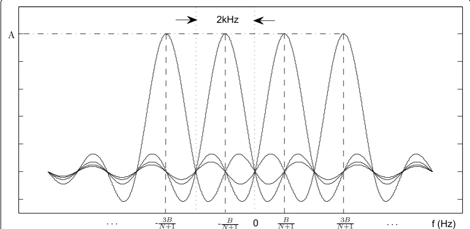
We propose to divide the entire 2.048 MHz band into 1,024 non-overlapping orthogonal subcarrier slots as shown in Figure 1, where each subcarrier slot has a null-to-null bandwidth of approximately 2 kHz. In our proposed design, the first and last eight subcarrier slots are left blank while the remaining 1,008 subcarrier slots are used to transmit the probing signals, namely, 42 unique subcarrier slots per SV. Due to the facts that (i) occupying the whole bandwidth results in a good
f (Hz) 0
· · · ·
A
B
N+1 N3+1B
2kHz
- 3B
N+1 -NB+1
ranging accuracy [16] and (ii) it is generally necessary to have all 24 SVs in GPS with more or less the same ran-ging accuracy since 4 to 12 SVs are usually visible at any point on earth and at any time, each group of 42 non-overlapping subcarrier slots is selected uniformly to cover the entire 2.048 MHz band.
DefineSIDas a number from 1 to 24 that is used to identify each SV. Define ID as an index set which is used to identify the subcarrier slots that are allocated to each SV. According to our design, an SV with the num-berSID, is allocated the index set,ID, as
ID= 8 + (SID−1) + (Sindex−1)× 24, (1)
whereSindex is an integer from 1 to 42, which denotes the specific subcarrier slot allocated to the Sth
IDSV.
Define S(f) as the continuous expression for the MC code in the frequency domain. It, in turn, can be sampled at f =±NB+1,±N3+1B ,. . .,±(NN−+11)B, N = 1024 and B= 1.023 MHz, which is shown in Figure 1 as dash lines. The resulting discrete expression is given by
S[k] =S
specifically, for the Sth
IDSV, we have
S[k] =
A, k∈ID
0, others (2)
where Ais a constant as shown in Figure 1 and the value ofAis determined by the transmitter power.
Equation (1) is explained further in Figure 2a, where 1,024 subcarrier slots are divided into 42 groups. Each group contains 24 subcarrier slots and the first and last eight subcarrier slots are left blank. Specifically, subcar-rier slots allocated to the kth, SV, are shown in Figure 2b, which includes thekth subcarrier of each group.
3 Ranging accuracy and SNR gain
The CRLB for time-based range estimation, Rˆ, can be expressed as [9,16]
energy;adenotes the complex-valued attenuation of the direct path; |·| denotes modulus; N0
2 is the PSD of the
additional white Gaussian noise (AWGN) in the propa-gation channel; |Na|2ξ
0/2 is the received SNR;cis the speed of light; B2 is the mean square bandwidth (MSB),
which can be approximated in a discrete form as
B2(≈a)(2πB
whereB= 1.023 MHz, and approximation (a) occurs due to the transformation from a continuous form to a discrete form, which will be verified by simulation. The PSD for the PN-based C/A code in GPS is a sinc square function [17-19], which implies that, S[k] in (4), is a sampled mainlobe of the sinc function. On the other hand, for our proposed design, the MSB can be further expressed as
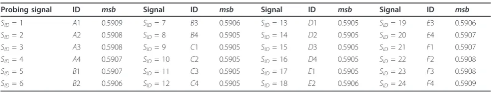
for the proposed MC code is calculated and illustrated in Table 1 for all SVs, i.e. SID= 1, 2, ..., 24. From Table 1, one can see that the proposed design has a MSB ran-ging from 0.5905 to 0.5909 MHz, implying that the 24 SVs have an approximately equal ranging accuracy. On the other hand, the MSB in MHz for the PN-based C/A code in GPS is obtained from (4) as 0.3427 MHz. One note to be pointed out is that the ID in Table 1 denotes the standard name in GPS and can be generally repre-sented as Lm, whereLis the orbit plane, from AtoF, and m is the specific SV, from 1 to 4 [12]. The SID
defined in this article is matched to the standard ID and shown in Table 1.
CRLB and the SNR for the proposed MC code,
respec-tively. Similarly, denote MSBc, CRLBc and
|a0|2ξ
N0/2
c as
the MSB, the CRLB and the SNR for the PN-based C/A code, respectively. The difference between the proposed MC code and the C/A code, in terms of CRLB for range estimation under an equal SNR, can be obtained as
CRLBs(dB)−CRLBc(dB)
= MSBc(dB)−MSBs(dB)
(a)
≈ −4.73(dB).
(6)
From another viewpoint, for a fixed ranging accuracy, the difference of the required SNR between the pro-posed design and the C/A code is obtained as
Which indicates that using the proposed MC code in GPS would lead to a 4.73 dB SNR gain compared to the current spread spectrum’s gold code.
4 Transmission and reception of the proposed MC code
As known, the data rate of the navigation message in cur-rent GPS is 50 bps while the bandwidth used for the pro-posed MC code is 1.024 MHz. The navigation message is
a telemetry message, and the data is transmitted in logical units called frames. For GPS, a frame is 1,500 bits long and takes 30 s to be transmitted. Each frame is divided into five subframes, 300 bits long per subframe. Subframes 1, 2 and 3 contain the high accuracy ephemeris and clock off set data. Subframes 4 and 5 contain the almanac data and some related health and configuration data [12].
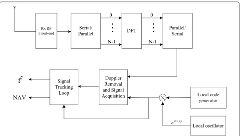
As shown in Figure 3, the proposed MC code is firstly modulated by the navigation message. Furthermore, the
1024
subcarrier slots
Group1
24
"
"
""
Group2
24
"
Group42
24
9
blank
8
"
"
f(Hz)
blank
8
1024
subcarrier slots
Group
1
"
""
"
Group
2
"
Group
42
blank
8
"
"
k+8
k+24*1+8
k+24*41+8
f(Hz)
blank
8
(a)
(b)
Figure 2Proposed MC code for GPS:(a)The entire 2.048 MHz band is uniformly divided into 1024 subcarrier slots, where the first and last 8 are left blank while the remaining 1008 are divided into 42 groups, each with 24 subcarriers.(b)42 subcarriers are allocated to thekthSV,k= 1,
2, ..., 24, which is made up of thekth subcarrier slot in each group.
Table 1 MSB in MHz, i.e. msb √MSB
2π MHz, for our proposed MC code withSID= 1, 2, ..., 24, and the PN-based C/A
code
Probing signal ID msb Signal ID msb Signal ID msb Signal ID msb
SID= 1 A1 0.5909 SID= 7 B3 0.5906 SID= 13 D1 0.5905 SID= 19 E3 0.5906
SID= 2 A2 0.5908 SID= 8 B4 0.5905 SID= 14 D2 0.5905 SID= 20 E4 0.5907
SID= 3 A3 0.5908 SID= 9 C1 0.5905 SID= 15 D3 0.5905 SID= 21 F1 0.5907
SID= 4 A4 0.5907 SID= 10 C2 0.5905 SID= 16 D4 0.5905 SID= 22 F2 0.5908
SID= 5 B1 0.5907 SID= 11 C3 0.5905 SID= 17 E1 0.5905 SID= 23 F3 0.5908
serial modulated data is converted to the parallel data and then transformed to the time domain by using inverse discrete Fourier transform (IDFT). Finally, the time-domain data is sent out by Tx RF Front-end. One note to be pointed out, every 20 MC-code cycles, i.e. 20 ms, are modulated by the same one bit of the naviga-tion message since the data rate of the MC code is much greater than that of the navigation message. The transmitted MC code is defined by Equations (1) and (2) and shown in Figure 2. The transmitted MC code is unique for a certain SV.
Figure 4 shows the block diagram of the reception of the proposed MC code in terms of range estimation. The time-domain data consisting of the modulated MC code is received by Rx RF Front-end. Furthermore, the serial modulated data is converted to the parallel data and then transformed to the frequency domain by using discrete Fourier transform (DFT).
The signal is received by Rx RF Front-end and down-converted to a serial baseband signal. The baseband sig-nal is sampled and converted to a parallel data. Passing by DFT, the parallel data is tranformed to frequency domain and passed into parallel/serial converter. The output serial signal, together with the local code genera-tor and local oscillagenera-tor, is then used for Doppler removal and acquisition [12]. Furthermore, via signal tracking process [12], both the partial delay estimation
ˆ
τ and NAV are obtained. Given τˆ and NAV, the range between transmitter and receiver can be obtained. One note to be pointed out is that the cross-correlation in signal acquistion and tracking is implemented in the fre-quency domain, which is given in [20].
5 NBI effect
In this section, define the POC as the probability that the NBI hits any part of the mainlobee of any of the subcarriers. The observation interval (OBI) is selected as 1 ms to evaluate NBI effect, leading to a null-to-null bandwidth of each subcarrier wnn = 2 kHz. The fre-quency range out of the available bandwidth 2B= 2.048 MHz, where the probing signal might be hit by a NBI, is wc = 42wnn kHz. This is the worst case since the greater the OBI, the narrower the subcarrier band, so the smaller the POC. The NBI effect is represented using POC, whereMuncorrelated NBIs are considered,
M = 1, 2, ..., 8, and each NBI is referred to be a fre-quency tone [21].
Therefore, the resulting POC,pc, can be obtained as
pc= 1−
1− wc
2B
M
= 1−0.959M. (8)
Based on (8), let us evaluate the probability that there are at least four visible non-collision SVs for one GPS receiver since GPS positioning requires four SVs. With-out loss of generality, assuming that there are eight SVs that are visible to one GPS receiver, the probability that there exists at most three visible non-colliding SVs is obtained as
pcc=
3
k=0
Ck81−pc
k
p8c−k
=
3
k=0
Ck80.959Mk[1−0.959M]8−k,
(9)
Serial/
Parallel IDFT
Parallel/ Serial NAV Message
#
0N-1
50bps MC code: Location wave
1.024 MHz
+1
-1
0
N-1
#
Tx RF
Front-end +1
-1
where Ck
8 denotes the number of combinations for
choosing k out of eight SVs. And the probability that there exists at least four visible non-colliding SVs, i.e. the probability of positioning success,Ps, is obtained as
Ps= 1−pcc= 1−
3
k=0
Ck80.959Mk[1−0.959M]8−k.(10)
For example, when M = 1, we have pc= w2Bc = 4.1%
and pcc=
3
k=0Ck8(1−pc)kpc8−k= 5.85×10⁻⁶, so Ps ≈
100%, indicating that the proposed MC code is robust against NBI.
6 Doppler effect
The motion of each SV causes a Doppler shift in the transmitted MC codes which can force a collision between the various transmitted groups of MC codes that are received by a GPS receiver. For a thorough ana-lysis on this collision, Appendix 1 analyzes the Doppler shift for an in-plane GPS receiver while Appendix 2 analyzes the Doppler shift for an off-plane GPS receiver in detail. In this section, the POC between MC codes due to Doppler shifts is theoretically explored. More specifically, we assume that a stationary GPS receiver is set to receive an MC code transmitted by SV “X”, and
measure the probability that its mainlobe collides with the mainlobe of MC codes transmitted by other SVs. In our analysis, we assume that the receiver has the maxi-mum possible visible region, i.e. a = 153oas shown in Figure 5 in Appendix 2, in all of the six orbital planes, i. e. that the receiver experiences the maximum possible Doppler shift from each one of the six orbital planes at the same time. This is a worst case scenario, which can be used as an upper bound on POC.
6.1 SV constellation
In GPS, the constellation of SVs in each orbit is deter-mined by true anomaly [12]. Since the eccentricity of orbits in GPS is less than 0.02 [12], which indicates a circle, the mean anomaly is approximately equal to the true anomaly. Therefore, by means of the mean anomaly [12], the constellation of SVs is shown in Figure 6. 6.1.1 Collision analysis between SVs in one orbit
Since the central angle between any two SVs in one orbit is fixed and the Doppler shift is monotonically decreasing with the central angle, then the Doppler dif-ference (DD) between any two visible SVs has a small variational range. Furthermore, since the subcarriers allocated to each SV are predetermined, thus the fre-quency spacing between the subcarriers without Doppler shift (FSBD) is fixed. As long as the frequency spacing
Rx RF Front-end
Doppler Removal and Signal
Acquisition Local code
generator
Local oscillator
ˆ
W
2 d
j f t e S
Serial/
Parallel
#
DFT0
N-1
Parallel/ Serial
#
0
N-1
Signal Tracking
Loop
NAV
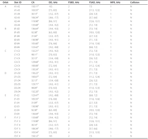
after Doppler shift (FSAD) is larger than the frequency resolution, the collision between subcarriers shall be avoided, otherwise, a collision shall occur. Table 2 takes all pairs of SVs in one orbit into consideration with respect to their relative central angle, their DD, FSBD, FSAD and finally their decision outcome. In Table 2, the central angle is obtained from the constellation of SVs, DD is obtained from simulation, FSAD is obtained
as the absolute value of summation of FSBD and DD, and the maximum frequency resolution (MFR) is selected as 1 kHz corresponding to an OBI of 1 ms. Even though, the central angles in Table 2 are less than the angle for the maximum possible visible range, one can conclude that there can never be any collision between groups of MC codes that are transmitted by SVs in one orbit.
Figure 5Visible range of an off-plane GPS receiver in terms of one SV (a)Representation of the visible rangeaof an off-plane GPS receiver;(b)the visible rangeaas a function of the elevation angleb.
A
98.09 92.38R 103.54R
R
6.1.2 Analysis On the visibility of an SV
It is essential to analyze the visibility of an SV by the recei-ver in order to obtain its probability of visibility and hence its POC with other SVs. Since the maximum possible visi-ble range for one SV by the receiver is 153o, according to the constellation shown in Figure 6, the visible region denoted by the central angle can be obtained. TakeB2 as an example, moving clockwise for a given receiver. When
B3 descends past the horizon,B2 is the only visible SV in orbitBuntilB4 ascends past the horizon, which corre-sponds to 130.98o+ 105.60o- 153o= 83.58o. Furthermore, take the combination ofC1 andC3 as an example, both moving clockwise for a given receiver. WhenC4 descends
past the horizon, onlyC1 andC3 in orbitCare visible to the receiver untilC1 descends past the horizon, which corresponds to 32.13o. Table 3 illustrates all possible com-binations of SVs as well as their corresponding visible regions and percentages. In Table 3, the probability of visi-bility (POV) is given as the ratio of the visible region to the whole circle since each SV is assumed to move with a con-stant velocity.
6.1.3 Approximation of visibility
From Table 3 that, one can see that the scenarios for all six orbits are similar. Firstly, the combinations of invisible SVs are exactly the same for all 6 orbits. Secondly, for all six orbits, the 2nd SV, the 3rd SV and the combination of Table 2 Collision analysis between SVs in each orbit for in-plane receivers, where Collision (S: Sure or N: Never) and CA: central angle
Orbit Slot ID CA DD, kHz FSBD, kHz FSAD, kHz MFR, kHz Collision
A A1-A2 150.11o -9.5 2 7.5 1 N
A1-A3 103.55o [7.5, 8.5] 4 [11.5, 12.5] 1 N
A1-A4 30.13o [-3.2, -0.7] 6 [2.8, 5.3] 1 N
A2-A3 106.34o [-8.6, -7.7] 2 [5.7, 6.6] 1 N
A2-A4 119.98o [8.6, 9.1] 4 [12.6, 13.1] 1 N
A3-A4 133.68o [-9.4, -9.2] 2 [7.2, 7.4] 1 N
B B1-B2 136.64o [-9.4, -9.3] 2 [7.3, 7.4] 1 N
B1-B3 92.38o [6.5, 8.0] 4 [10.5, 12.0] 1 N
B1-B4 31.04o [-3.3, -0.7] 6 [2.7, 5.3] 1 N
B2-B3 130.98o [-9.3, -9.1] 2 [7.1, 7.3] 1 N
B2-B4 105.60o [7.6, 8.6] 4 [11.6, 12.6] 1 N
B3-B4 123.42o [-9.2, -8.8] 2 [6.8, 7.2] 1 N
C C1-C2 132.21o [-9.3, -9.2] 2 [7.2, 7.3] 1 N
C1-C3 98.11o [7.0, 8.3] 4 [11.0, 12.3] 1 N
C1-C4 32.13o [-3.4, -0.8] 6 [2.6, 5.2] 1 N
C2-C3 129.68o [-9.3, -9.1] 2 [7.1, 7.3] 1 N
C2-C4 100.08o [7.2, 8.4] 4 [11.2, 12.4] 1 N
C3-C4 130.24o [-9.3, -9.1] 2 [7.1, 7.3] 1 N D D1-D2 130.22o [-9.3, -9.1] 2 [7.1, 7.3] 1 N
D1-D3 100.07o [7.2, 8.4] 4 [11.2, 12.4] 1 N
D1-D4 32.13o [-3.4, -0.8] 6 [2.6, 5.2] 1 N
D2-D3 129.71o [-9.3, -9.1] 2 [7.1, 7.3] 1 N
D2-D4 98.09o [7.0, 8.3] 4 [11.0, 12.3] 1 N
D3-D4 132.20o [-9.3, -9.2] 2 [7.2, 7.3] 1 N
E E1-E2 123.47o [-9.2, -8.8] 2 [6.8, 7.2] 1 N
E1-E3 105.55o [7.6, 8.6] 4 [11.6, 12.6] 1 N
E1-E4 31.09o [-3.3, -0.7] 6 [2.7, 5.3] 1 N
E2-E3 130.98o [-9.3, -9.1] 2 [7.1, 7.3] 1 N
E2-E4 92.38o [6.5, 8.0] 4 [10.5, 12.0] 1 N
E3-E4 136.64o [-9.4, -9.3] 2 [7.3, 7.4] 1 N F F1-F2 133.68o [-9.4, -9.2] 2 [7.2, 7.4] 1 N
F1-F3 119.98o [8.6, 9.1] 4 [12.6, 13.1] 1 N
F1-F4 30.14o [-3.2, -0.7] 6 [2.8, 5.3] 1 N
F2-F3 106.34o [-8.6, -7.7] 2 [5.7, 6.6] 1 N
F2-F4 103.54o [7.5, 8.5] 4 [11.5, 12.5] 1 N
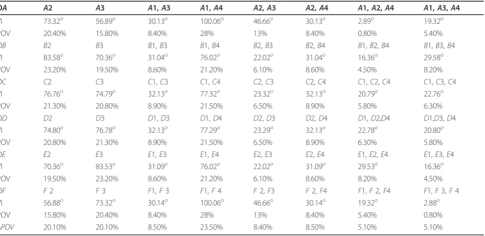
the 1st and 4th SV have similarly the largest visible inter-val, which corresponds to a POV of approximately 20%. Thirdly, for all orbits, the majority of combinations of the 1st and 3rd SV, the 2nd and 3rd SV, the 2nd and 4th SV, the 1st, 2nd and 4th SV, and the 1st, 3rd and 4th SV have a small POV that is lower than 10%. In other words, even though they are different in some ways, e.g. the combina-tions ofA2 andA3, as well asF2 andF3 have about 13% POV, the scenarios for all six orbits are still very similar. Therefore, to simplify the analysis of the POC, the average visible interval and APOV in Table 3, are used for all six orbits. This is equivalent to using the average constellation for one orbit, which is shown in Figure 7, instead of the six constellations which are shown in Figure 6.
6.2 Theoretical procedure for calculating POC
Since there is no collision between SVs in one orbit, the in-orbit‘adjacencies’fdo not exist and the number of‘ adja-cencies’is thus reduced. To calculate the POC: denote by
M the number of‘adjacencies’ of the desired SV“X"; denote by, pMk,k= 1, 2, 3, 4, the probability of havingk ’adjacencies’to“X”, which is ana prioriprobability; denote by, pvkj, 1≤j≤k, the probability of visibility ofj’
adjacen-cies’to“X”whenM=k, which is also ana priori probabil-ity; denote by,pk(collision|jvisible), the POC under the condition that there arejvisible‘adjacencies’to“X”when
M=k, which is a conditional probability.
WhenM= 1 with a probability pM1, the procedure for calculating pc1, which is defined as the POC when there
is only one ‘adjacency’, is as follows: (1) calculate the
probability of visibility pv11of this‘adjacency’; (2) calcu-late the conditional probability p1 (collision|1 visible), which is the POC when the‘adjacency’of SV“X” is also visible to the GPS receiver; (3) calculate pc1 by removing
the condition with respect to the visibility:
pc1=p1(collision|1 visible)pv11. (11) Similarly, When M = 2 with a probability pM2,pc2,
which is defined as the POC when there are two‘ adja-cencies’, can be obtained as
Table 3 Visibility analysis for the fixed in-plane GPS receiver, where VI: Visible interval, POV: Probability of Visibility, APOV: Average Probability of Visibility and OX: OrbitX, whereXdenotesA,B,C,D,EorF
OA A2 A3 A1,A3 A1,A4 A2,A3 A2,A4 A1,A2,A4 A1,A3,A4
VI 73.32o 56.89o 30.13o 100.06o 46.66o 30.13o 2.89o 19.32o POV 20.40% 15.80% 8.40% 28% 13% 8.40% 0.80% 5.40% OB B2 B3 B1,B3 B1,B4 B2,B3 B2,B4 B1,B2,B4 B1,B3,B4 VI 83.58o 70.36o 31.04o 76.02o 22.02o 31.04o 16.36o 29.58o POV 23.20% 19.50% 8.60% 21.20% 6.10% 8.60% 4.50% 8.20% OC C2 C3 C1,C3 C1,C4 C2,C3 C2,C4 C1,C2,C4 C1,C3,C4 VI 76.76o 74.79o 32.13o 77.32o 23.32o 32.13o 20.79o 22.76o
POV 21.30% 20.80% 8.90% 21.50% 6.50% 8.90% 5.80% 6.30% OD D2 D3 D1,D3 D1,D4 D2,D3 D2,D4 D1,D2,D4 D1,D3,D4 VI 74.80o 76.78o 32.13o 77.29o 23.29o 32.13o 22.78o 20.80o
POV 20.80% 21.30% 8.90% 21.50% 6.50% 8.90% 6.30% 5.80% OE E2 E3 E1,E3 E1,E4 E2,E3 E2,E4 E1,E2,E4 E1,E3,E4 VI 70.36o 83.53o 31.09o 76.02o 22.02o 31.09o 29.53o 16.36o POV 19.50% 23.20% 8.60% 21.20% 6.10% 8.60% 8.20% 4.50% OF F2 F3 F1,F3 F1,F4 F2,F3 F2,F4 F1,F2,F4 F1,F3,F4 VI 56.88o 73.32o 30.14o 100.06o 46.66o 30.14o 19.32o 2.88o POV 15.80% 20.40% 8.40% 28% 13% 8.40% 5.40% 0.80%
APOV 20.10% 20.10% 8.50% 23.50% 8.40% 8.50% 5.10% 5.10%
Average
constellation
1
4
2
3
R
30
R
105
R
120
R
105
pc2=p2(collision|1 visible)pv21 +p2(collision|2visible)pv22;
(12)
when M = 3 with a probability pM3,pc3, which is defined as the POC when there are three ‘adjacencies’, can be obtained as
pc3=p3(collision|1 visible)pv31 +p3(collision|2 visible)pv32 +p3(collision|3 visible)pv33;
(13)
WhenM= 4 with a probability pM4, the procedure for calculating pc4, which is defined as the POC when there are four‘adjacencies’can be obtained as
pc4=p4(collision|1 visible)pv41 +p4(collision|2 visible)pv42 +p4(collision|3 visible)pv43 +p4(collision|4 visible)pv44.
(14)
The overall POC,pc, is represented by removing the condition with respect toM:
pc=
4
k=1
pckpMk. (15)
6.3A prioriprobability pvkj
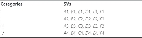
Each SV has a unique allocation of subcarriers, and each subcarrier has different neighboring sub-carriers, some of which are co-orbital while others are not. We already know that, no collision occurs between co-orbital sub-carriers. Therefore, the four SVs in one orbit have a dif-ferent number of‘adjacencies’and correspondingly have different probabilities of collision at any given time. However, all first SVs in each one of the 6 orbits have the same scenario and the same number of‘adjacencies’, which we cluster into Category I; all second SVs have the same scenario and the same number of‘adjacencies’, which we cluster into Category II; all third SVs have the same scenario and the same number of ‘adjacencies’, which we cluster into Category III; all fourth SVs have the same scenario and the same number of‘adjacencies’, which we cluster into Category IV. All of the SVs are therefore clustered into one of the four categories and are shown in Table 4.
The desired SV would locate in one of these four Categories. The following parts will consider all cases that the desired SV lies in a specific Catogory. In order to obtain the priori probability pvkj,
- the first step is to get the number of the‘adjacency’ of the desired SV. Since the number of ‘adjacencies’is evidently changing with the Doppler shift of the desired
SV, the number of ‘adjacencies’will be obtained with the corresponding Doppler interval of the desired SV.
- For the case that the desired SV has one‘adjacency’, referring to Table 3, the visiable range of this‘adjacency’ in the percentage can be obtained. This value is pv11.
- For the case that the desired SV has two ‘ adjacen-cies’, referring to Table 3, the visible range of either of two‘adjacencies’can be obtained and this value leads to
pv21. And the visible range of both‘adjacencies’obtained by reffereing to Table 3 will lead to pv22.
- For the case that the desired SV has three ‘ adjacen-cies’, referring to Table 3, the visible range of any of three ‘adjacencies’ can be obtained and this value leads to pv31. The visible range of any two ‘adjacencies’
obtained by reffereing to Table 3 will lead to pv32. And the visible range of all three ‘adjacencies’ obtained by reffereing to Table 3 will lead to pv33.
- For the case that the desired SV has four ‘ adjacen-cies’, referring to Table 3, the visible range of any of four‘adjacencies’can be obtained and this value leads to
pv41. The visible range of any two‘adjacencies’obtained by reffereing to Table 3 will lead to pv42. The visible
range of any three‘adjacencies’obtained by reffereing to Table 3 will lead to pv43. And the visible range of all
four‘adjacencies’obtained by reffereing to Table 3 will lead to pv44.
The details are presented as follows. 6.3.1 Category I
Let the desired SV be in Category I and be referred to asB1. WhenB1 suffers from a Doppler shift, fDX, which
falls in the interval of [-4.75,-3.25] kHz, we have four
‘adjacencies’toB1 which might collide withB1: SVsA1,
A2,A3 andA4. More specifically, because the subcarrier spacing betweenB1 andA4 is 2 kHz,A4 will completely collide with B1 if the Doppler shift on A4 is
fDX+ 2kHz. Similarly,A3 will completely collide with B1 if the Doppler shift on A3 is fDX+ 4kHz. A2 will
also completely collide withB1 if the Doppler shift on A2 is fDX+ 6kHz. Finally, A1 will also completely
col-lide with B1 if the Doppler shift onA1 is fDX+ 8kHz.
When the Doppler shift on B1 falls in the interval of [-3.25, -1.25] kHz, A1, A2 andA3 are its ‘adjacencies’, however, A1 is not capable of colliding with B1 even Table 4 24 SVs are clustered into four categories, each of which contains six SVs
Categories SVs
with the biggest possible Doppler shift. When B1 suffers from a Doppler shift which falls in the interval of [-1.25, 0.75] kHz,A3 andA4 are its‘adjacencies’. WhenB1 suf-fers from a Doppler shift which falls in the interval of [0.75, 2.75] kHz, onlyA4 is its‘adjacency’. When the Doppler shift on B1 is in the interval of [2.75, 3.25] kHz, no ‘adjacencies’ exist and so no collision can take place. Finally, when the Doppler shift onB1 belongs to the interval [3.25, 4.75] kHz,C1 becomes its‘adjacency’ and can collide with it. Table 5 shows the number of
‘adjacencies’of the desired SV in Category I with respect to fDX.
Referring to the average visible interval, the a priori
probabilities can be obtained. Firstly, if
fDX ∈[3.25, 4.75] kHz, onlyC1 is the‘adjacency’ofB1.
Looking into Table 3,C1 is visible in the form of the following four combinations: {C1, C3}, {C1, C4}, {C1,
C2,C4}, or {C1,C3,C4}. In total, the visible range for
C1 is 8.5% + 23.5% + 5.1% × 2 = 42.2%. Similarly, when
fDX∈[0.75, 2.75] kHz, the visible range is also 42.2%.
Overall, pv11 = 42.2%.
When fDX∈[−1.25, 0.75]kHz, there are two ‘
adja-cencies’ for B1: A3 and A4. Looking into Table 3, exactly one‘adjacency’, A3, is visible in the following three forms:A3 alone, the combinations of {A1,A3} or {A2, A3}. In this case, A3 has a visible range of 37%. Similarly, exactly one ‘adjacency’, A4, is visible in the following three forms: the combinations of {A1, A4}, {A2,A4}, or {A1,A2,A4}. In this case,A4 has a visibility range of 37.1%. Finally, exactly two ‘adjacencies’are visi-ble in the form of the combination of {A1, A3, A4}, which corresponds to a visibility range of 5.1%. Thus, it is concluded that pv21 = 74.1% and pv22 = 5.1%.
When fDX ∈[−3.25,−1.75]kHz, there are three ‘adjacencies’A2,A3 andA4 of the desired SVB1. Look-ing into Table 3, exactly one‘adjacency’A2 is visible in the form ofA2 alone, which corresponds to a visibility range of 20.1%. Similarly, exactly one‘adjacency’A3 is
visible in the form ofA3 alone or as a combination of {A1, A3}, which corresponds to a visibility range of 28.6%. Also, exactly one ‘adjacency’A4 is visible in the form of the combination of {A1,A4}, which corresponds to a visibility range of 23.5%. Exactly two ‘adjacencies’
A2 and A3 are visible with a visibility range of 5.1%. Exactly two ‘adjacencies’ A2 and A4 are visible in the form of the two combinations of {A2, A4} or {A1, A2,
A4}, which correspond to a visibility range of 13.6%. Exactly two ‘adjacencies’ A3 and A4 are visible in the form of the combination of {A1,A3,A4}, which corre-sponds to a visibility range of 5.1%. Exactly three‘ adja-cencies’A2,A3 and A4 are always invisible. Thus, it is concluded that pv31 = 72.2%, pv32 = 23.8% and
pv33 = 0%.
When fDX∈[−4.75,−3.25]kHz, there are four ‘
adja-cencies’forB1:A1,A2,A3 and A4. Looking into Table 3, exactly one‘adjacency’ is visible in the form ofA2 or
A3, which corresponds to the visibility range of 40.2%. Exactly two ‘adjacencies’ are visible in the form of {A1,
A3}, {A1,A4}, {A2,A3} or {A2, A4}, which correspond to a visibility range of 48.9%. Exactly three‘adjacencies’ are visible in the form of {A1,A2,A4} or {A1,A3,A4}, which correspond to a visibility range of 10.2%. One should note that it is impossible that exactly four‘ adja-cencies’are visible simultaneously. Thus, it is concluded that pv41= 40.2%, pv42 = 48.9%, pv43 = 10.2% and
pv44= 0%.
6.3.2 Category II
Similarly, takingB2 as an example of the desired SV, the number of ‘adjacencies’ ofB2 with respect to fDX is
shown in Table 6.
When fDX∈[1.25, 3.25]kHz, only C1 is the ‘
adja-cency’ for B2. Similar to Category I, we have
pv11= 42.2%. When fDX∈[−1.25, 0.75]kHz, there is
also only one‘adjacency’to B2:A4. Following a similar analysis, it is concluded that is also equal to
Table 5 The changing process of the number of‘adjacencies’of the desired SV‘’X’’in Category I (i.e. the SVB1) with respect to Doppler shift on the SV‘’X’’
fDX,kHz [-4.75, -3.25] [-3.25, -1.25] [-1.25, 0.75] [0.75, 2.75] [2.75, 3.25] [3.25, 4.75]
M 4 3 2 1 0 1
’adjacencies’ A1,A2,A3,A4 A2,A3,A4 A3,A4 A4 NULL C1
Table 6 The changing process of the number of‘adjacencies’of the desired SV‘’X’’in Category II (i.e. the SVB2) with respect to Doppler shift on the SV‘’X’’
fDX,kHz [-4.75, -3.25] [-3.25, -1.25] [-1.25, 0.75] [0.75, 1.25] [1.25, 3.25] [3.25, 4.75]
M 3 2 1 0 1 2
fDX. Consequently, the overalla prioriprobability forM
= 1 is also 42.2%.
When fDX∈[3.25, 4.75] kHz, C1 and C2 are its ‘adjacencies’. Referring to Table 3, exactly one ‘ adja-cency’ C1 is visible in the form of the combinations: {C1,C3}, {C1,C4}, or {C1,C3,C4}, which corresponds to a visibility range of 37.1%. Exactly one‘adjacency’C2 is visible in the form of C2 alone, or in the combina-tions of {C2, C3} or {C2,C4}, which corresponds to a visibility range of 37%. Exactly two ‘adjacencies’ are simultaneously visible in the form of the combination of {C1,C2,C4}, which corresponds to a visibility range of 5.1%. Thus, it is concluded that pv21 = 74.1% and
pv22 = 5.1%. When fDX ∈[−3.25,−1.25]kHz, A3 and A4 are the‘adjacencies’of B2. As analyzed in Category I, the same values of pv21 = 74.1% and pv22 = 5.1% are obtained. Overall speaking, whenM = 2, the a priori
probabilities are pv21 = 74.1% and pv22= 5.1%.
When fDX ∈[−4.75,−3.25]kHz, there are three ‘adjacencies’A2,A3 andA4 of the desired SVB2. With the same analysis shown in Category I, one can con-clude that pv31 = 72.2%, pv32 = 23.8% and pv33 = 0%.
Because B2 has at most three‘adjacencies’, it is evident that pv41=pv42 =pv43 =pv44 = 0%.
6.3.3 Category III
Similarly, takingB3 as an example of the desired SV, the number of ‘adjacencies’ ofB3 with respect to fDX is
shown in Table 7.
When fDX ∈[−0.75, 1.25]∪[−3.25,−1.25] kHz, only C1 or A4 is the‘adjacency’ of the desired SV B3. As shown in Category II, it is obtained that pv11 = 42.2%.
When fDX ∈[1.25, 3.25]kHz, C1 and C2 are the ‘adjacencies’of the desired SVB3. As analyzed in Cate-gory II, it is provided that pv21 = 74.1% and
pv22 = 5.1%. When fDX∈[−4.75,−3.25]kHz, there are
also two‘adjacencies’: A3 andA4, and it is shown that also pv21 = 74.1% and pv22 = 5.1%. Overall speaking,
when M= 2, thea priori probabilities are pv21 = 74.1% and pv22 = 5.1%.
When fDX ∈[3.25, 4.75] kHz, C1,C2 andC3 are the ‘adjacencies’of the desired SVB3. Referring to Table 3, exactly one ‘adjacency’ C1 is visible in the form of the combination {C1,C4}, which corresponds to a visibility range of 23.5%. Exactly one ‘adjacency’C2 is visible in the form of C2 alone or the combination {C2, C4}, which corresponds to a visibility range of 28.6%. Exactly one ‘adjacency’ C3 is visible in the form ofC3 alone, which corresponds to the visibility range of 20.1%. Exactly two ‘adjacencies’ C1 and C2 are visible in the form of the combinations {C1,C2, C4}, which corre-sponds to a visibility range of 5.1%. Exactly two‘ adja-cencies’ {C2, C3} are visible with a visibility range of 8.4%. Exactly two‘adjacencies’C1 and C3 are visible in the form of the combinations of {C1, C3} or {C1, C3,
A4}, which correspond to a visibility range of 13.6%. Exactly three ‘adjacencies’ C1, C2 andC3 are always invisible. Thus, it is concluded that pv31 = 72.2%,
pv32= 23.8% and pv33 = 0%. Also since B3 has at most
three ‘adjacencies’, it is evident that
pv41 =pv42 =pv43 =pv44 = 0%.
6.3.4 Category IV
Similarly, takingB4 as an example of the desired SV, the number of ‘adjacencies’ ofB4 with respect to fDX is
shown in Table 8.
When fDX∈[−4.75,−3.25]∪[−2.75,−0.75] kHz,
onlyC1 or A4 are the‘adjacencies’of B4. As shown in Category III, it is obtained that pv11= 42.2%. When
fDX ∈[−0.75, 1.25] kHz, C1 and C2 are the ‘
adjacen-cies’of B4. As shown in Category III, pv21 = 74.1% and
pv22 = 5.1%. When fDX∈[1.25, 3.25]kHz, the SVs C1, C2 and C3 are the ‘adjacencies’ ofB4. As shown in Category III, pv31 = 72.2%, pv32 = 23.8% and pv33 = 0%. When fDX ∈[3.25, 4.75] kHz, there are four‘
adjacen-cies’C1,C2,C3 andC4 of the desired SVB4, which is the same as the four ‘adjacencies’A1, A2, A3 and A4.
Table 7 The changing process of the number of‘adjacencies’of the desired SV‘’X’’in Category III (i.e. the SVB3) with respect to Doppler shift on the SV‘’X’’
fDX,kHz [-4.75, -3.25] [-3.25, -1.25] [-1.25, -0.75] [-0.75, 1.25] [1.25, 3.25] [3.25, 4.75]
M 2 1 0 1 2 3
’adjacencies’ A3,A4 A4 NULL C1 C1,C2 C1,C2,C3
Table 8 The changing process of the number of‘adjacencies’of the desired SV‘’X’’in Category IV (i
fDX,kHz [-4.75, -3.25] [-3.25, -2.75] [-2.75, -0.75] [-0.75, 1.25] [1.25, 3.25] [3.25, 4.75]
M 1 0 1 2 3 4
As shown in Category I, it is obtained that
pv42= 48.9%, pv42 = 48.9%, pv43 = 10.2% and
pv44= 0%.
6.4A prioriprobability pMk
The desired SV would locate in one of these four Cate-gories. The priori probability pMk is different when the
desired SV lies in a different Category. In a specific Category,
- the first step is to figure out the Doppler interval when the desired SV has one‘adjacency’and to calculate the probability that the desired SV has a Doppler shift within this interval. This percentage leads to the value of pM1.
-The second step is to figure out the Doppler interval when the desired SV has two‘adjacencies’and to calcu-late the probability that the desired SV has a Doppler shift within this interval. This percentage leads to the value of pM2.
- The third step is to figure out the Doppler interval when the desired SV has three‘adjacencies’and to cal-culate the probability that the desired SV has a Doppler shift within this interval. This percentage leads to the value of pM3.
- The last step is to figure out the Doppler interval when the desired SV has four‘adjacencies’and to calcu-late the probability that the desired SV has a Doppler shift within this interval. This percentage leads to the value of pM4.
The details are presented as follows. 6.4.1 Category I
Looking into Table 5, there is one ‘adjacency’ when
fDX∈[0.75, 2.75]∪[3.25, 4.75]kHz. By means of the
PDF of the Doppler shift, its integration over the speci-fied interval is obtained as pM1 = 41.3%. Similarly, there are two ‘adjacencies’ when fDX∈[−1.25, 0.75]kHz, pM2 = 12.2%. There are three ‘adjacencies’ when
pM3 = 14.5%, pM3 = 14.5%. There are four ‘ adjacen-cies’when fDX∈[−4.75,−3.25]kHz, pM4 = 27.8%. 6.4.2 Category II
Looking into Table 6, there is one ‘adjacency’ when
fDX ∈[−1.25, 0.75]∪[1.25, 3.25] kHz. Similar to
Category I, we have pM1 = 26.8%. There are two ‘
adja-cencies’ when
pM2 = 42.3%, pM2 = 42.3%. There are three‘
adjacen-cies’ when fDX∈[−4.75,−3.25]kHz, pM3= 27.8%. Since there are at most three ‘adjacencies’for SVs in this Category, pM4 = 0%.
6.4.3 Category III
Looking into Table 7, there is one ‘adjacency’ when
fDX ∈[−3.25, −1.25]∪[−0.75, 1.25] kHz, we have
Looking into Table 8, there is one ‘adjacency’ when
pM1 = 41.3%, pM1 = 41.3%. There are two‘adjacencies’ when fDX∈[−0.75, 1.25] kHz, pM2 = 12.2%. There are three ‘adjacencies’ when fDX ∈[1.25, 3.25]kHz, pM3= 14.5%. There are four ‘adjacencies’ when
pM3= 27.8%, pM3 = 27.8%.
6.5 Conditional probabilitypk(collision|jvisible)
The conditional probability is related with the null-to-null bandwidth of each subcarrier,wnn. The smaller the OBI, the bigger the bandwidth, the larger the condi-tional probability. We consider two cases: (1) the OBI is equal to 1 ms, i.e. the null-to-null bandwidth of each subcarrier is equal to 2 kHz; and (2) the OBI is equal to 20 ms, i.e. the null-to-null bandwidth of each subcarrier is equal to 0.1 kHz.
The desired SV would locate in one of these four Categories. In each Catogory, in order to obtain the conditional probability pk(collision|jvisible), the first step is to determine the ‘adjacencies’of the desired SV and the corresponding Doppler shifts when any of them is visible. Assuming the center frequency of the desired SV without Doppler shift is at zero, the center frequency of the desired SV after considering Doppler shift can be obtained. Furthermore, the center frequency of the
‘adjacencies’of the desired SV safter considering Dop-pler shift can be obtained based on the subcarrier space of the
p1(collision|1 visible) = 3.25
transmitting signal of the ‘adjacencies’and the desired SV. The POC at a specific Doppler bin of the desired SV can then be calculated based on the non-uniform distribution of the Doppler shift. Finally, based on this POC at a specific Doppler bin, the conditional probabil-ity pk(collision|j visible) can be obtained. The details are presented as follows.
6.5.1 Category I
When fDX∈[3.25, 4.75] kHz, C1 is the unique‘
adja-cency’ofB1. Referring to Table 3, the Doppler shift on the visibleC1 belongs to the interval [-4.75, 4.75] kHz. So, relative toB1 without Doppler, the shiftedC1 lies in [8 -4.75, 8 + 4.75] kHz since the subcarrier spacing between
withC1 cannot be avoided, and the magnitude of the colli-sion is determined by wnn. At each fDX, the POC is
obtained as fDX−8+
wnn 2
fDX−8−wnn 2
p(fDC1)dfDC1, where fDC1 is the
PDF of the Doppler shift on the‘adjacency’C1. However, a different fDX corresponds to a different POC due to the
non-uniform distribution of the Doppler shift. Based on the distribution of fDX, denoted by p(fDX), we have
p1(collision|1 visible,fDX ∈ [3.25, 4.75])
=
fDX−8+w2nn
fDX−8−w2nn
pfDC1
dfDC1,
(16)
and
pfDX|fDX ∈ [3.25, 4.75]
= p(fDX)
3.25
4.75 p(fDX)dfDX
. (17)
So, the average POC when fDX ∈[3.25, 4.75] kHz
can be expressed as Equation (18). Based on (18), and on Figures 8, we have p1 (collision|1 visible) = {24.3%, 1.42%}.g
When fDX∈[−1.25, 0.75]kHz, there are two‘
adjacen-cies’:A3 andA4. IfA3 is visible whileA4 is not, looking into Table 3, the Doppler shift onA3 is in [-4.75, 4,43] kHz and so, relative toB1,A3 lies in [-8.75, 0.43] kHz. When fDX ∈ [−1.25, 0.43] kHz, a collision occurs in
the same way as above. In this case, the POC is obtained as {27.3%, 1.28%}. Thus, the integrated POC is {22.9%, 1.08%}. IfA4 is visible whileA3 is not, looking into Table 3, the Doppler shift onA4 is in [-4.43, 4, 75] kHz and so, relative toB1,A4 lies in [-6.73, 2.75] kHz and the POC is approximately {15.8%, 0.78%}. Considering the relative visibility range, the resulting conditional POC for one visible‘adjacency’is p2 (collision|1 visible) = {19.4%, 0.92%}. If bothA3 andA4 are visible, they lie respectively in [0.43, 0.75] and [-6.75, -6.43] kHz relative toB1. It is evident thatB1 may collide withA3 while not withA4. When fDX ∈ [−1.25, 0.43] kHz, no collision occurs.
When fDX ∈ [0.43, 0.75] kHz, the collision occurs with
the following probability: {100%, 26.8%}. Finally, the inte-grated conditional POC for two visible‘adjacencies’isp2 (collision|2 visible) = {29.8%, 4.20%}.
When fDX ∈[−3.25,−1.25]kHz, there are three‘
adja-cencies’:A2,A3 andA4. If exactlyA2 is visible, it lies in [-7.98, 1.57] kHz, the corresponding POC is {40.6%,
0 20 40 60 80 100 120 140 160 180
−5 −4 −3 −2 −1 0 1 2 3 4 5
Central angle, γ
Doppler (kHz)
1.90%}. If exactlyA3 is visible, it lies in [-8.43, 0.43] kHz, and the POC is {18.5%, 0.91%}. If exactlyA4 is visible,A4 lies in [-6.43, -0.02] kHz, and the corresponding POC is {25.1%, 1.24%}. Taking the visibility range into considera-tion, the conditional POC for one visible‘adjacency’isp3 (collisionj1 visible) = {26.8%, 1.29%}. WhenA2 andA3 are visible whileA4 is not,A2 lies in [-1.57, -1.25] kHz, which leads to the integrated POC {26.0%, 3.75%}. Any other combinations of two visible‘adjacencies’cannot cause collision. Taking the visibility range into considera-tion,p3(collision|2 visible) = {5.9%, 0.8%}. Additionally, since the condition of three simultaneously visible‘ adja-cencies’is false, calculating the POC under this condition is meaningless because its contribution to the collision is 0 when removing the condition.
When fDX ∈[−4.75,−3.25]kHz, there are four‘
adja-cencies’:A1,A2,A3 andA4. When exactly one is visible,
A2 and A3 lie in [-7.98, -1.57] and [-8.43, -2.02] kHz, respectively. So, we havep4(collision|1 visible) = {26.3%, 1.29%}. The scenarios of two visible‘adjacencies’cannot cause collision except forA1 andA4, where A1 lies in [-9.98, -3.57]kHz, leading to a collision probability of {43.9%, 2.00%}, andA4 lies in [-6.43, -0.02] kHz, leading to a collision probability of {29.9%, 1.46%}. Since no collision occurs between SVs in one orbit, whenA1 collides withB1,
A4 doesn’t. Also, whenA4 collides withB1,A1 doesn’t. So the POC for such scenario is {73.8%, 3.46%}. Averaged by the visible range,p4(collision|2 visible) = {35.4%, 1.66%}. For the scenario of three visible‘adjacencies’ofA1,A2 and
A4,A1 lies in [-3.57, -3.25]kHz, which provides a collision probability of {20.5%, 2.90%}, while the scenario ofA1,A3 andA4 cannot cause collision. So, we havep4(collision|3 visible) = {10.2%, 1.45%}. Additionally, the condition of four simultaneously visible‘adjacencies’is false and its contribu-tion to the collision is 0 when removing the condicontribu-tion. 6.5.2 Category II
When fDX∈[−1.25,−0.75]kHz, there is one ‘
adja-cency’ A4, and the corresponding POC is equal to {23.8%, 1.57%}. When fDX ∈[1.25, 3.25]kHz, there is
one‘adjacency’C1, and the POC is {23.5%, 1.49%}. Con-sidering the occurrence probability, 12.2 and 14.5% for
fDX∈[−1.25,−0.75]kHz and fDX ∈[1.25, 3.25]kHz,
respectively, the average conditional POC is obtained as
p1(collision|1 visible) = {23.6%, 1.53%}.
When fDX∈[3.25, 4.75] kHz, there are two‘
adjacen-cies’:C1 andC2. When onlyC1 is visible, it lies in [1.25, 10.43] kHz relative toB2, and the corresponding POC is {15.7%, 0.77%}. When onlyC2 is visible, it lies in [3.57, 12.57] kHz relative toB2, and the corresponding POC is {24.8%, 1.15%}. Taking the visibility range into considera-tion, the resulting POC for one visible‘adjacency’is {20.3%, 0.96%}.
When bothC1 andC2 are visible,C2 lies in [3.25, 3.57] kHz, the corresponding POC is {20.5%, 3.00%}, whileC1 cannot cause any collisions. So, the resulting conditional POC for two visible‘adjacencies’is {20.5%, 3.00%}. On the other hand, when fDX∈[−3.25,−1.25]kHz, there are
two‘adjacencies’:A3 andA4, and the POC is {19.4%, 0.92%} for one visible‘adjacency’and {26.0%, 3.75%} for two simultaneously visible‘adjacencies’. Also, the occur-rence probability for fDX ∈[3.25, 4.75] kHz and fDX ∈[−3.25,−1.25]kHz is 27.8 and 14.5%, respectively.
Overall,p2(collision|1 visible) = {20.0%, 0.95%}. andp2 (collision|2 visible) = {22.5%, 3.26%}.
When fDX ∈[−4.75,−3.25]kHz, there are three ‘adjacencies’:A2,A3 and A4. When onlyA2 is visible, the POC is {43.9%, 2.00%}. When onlyA3 is visible, the POC is {18.5%, 0.91%}. When only A4 is visible, the POC is {24.9%, 1.23%}. Thus, we have p3 (collision|1 visible) = {27.6%, 1.32%}. When A2 and A3 are visible whileA4 is not, the POC is {20.5%, 2.90%}, while other combinations of two SV’s being visible cannot lead to a collision. Thus,p3 (collision|2 visible) = {4.5%, 0.62%}. Additionally, the condition of three simultaneously visi-ble ‘adjacencies’is false, so its contribution to the POC is 0 when removing this condition.
Since the condition of four‘adjacencies’is also false, its contribution to the POC is also 0 when removing this condition.
6.5.3 Category III
When fDX∈[−3.25,−1.25]kHz, there is one ‘
adja-cency’ A4, and the corresponding POC is equal to {23.5%, 1.49%}. When fDX∈[−0.75, 1.25] kHz, there is
one‘adjacency’C1, and the POC is {23.8%, 1.57%}. Also, the occurrence probability for fDX∈[−3.25,−1.25]kHz
and fDX ∈[−0.75, 1.25] kHz is 14.5 and 12.2%,
respec-tively. So, the average conditional POC isp1(collision|1 visible) = {23.6%, 1.53%}.
When fDX ∈[−4.75,−3.25]kHz, there are two‘
adja-cencies’:A3 andA4. When only A3 is visible, the POC is {24.9%, 1.13%}. When only A4 is visible, it is {15.7%, 0.77%}. So, the average value is {20.3%, 0.95%}. When bothA3 andA4 are visible, the POC is {20.5%, 3.00%}. When fDX∈[1.25, 3.25]kHz, there are two ‘
adjacen-cies’: C1 and C2. When only C1 is visible, the POC is {15.7%, 0.77%}. When only C2 is visible, it is {24.1%, 1.13%}. Thus, taking the visible range into consideration, we have {19.9%, 0.95%}. When bothC1 andC2 are visi-ble, the POC is {20.5%, 3.15%}. Also, the occurrence probability for fDX∈[−4.75,−3.25]kHz and fDX ∈[1.25, 3.25]kHz is 27.8 and 14.5%, respectively.
(collision|2 visible) = {20.5%, 3.05%} for two visible 2.37%}. Taking the visibility range into consideration, the corresponding conditional POC can be obtained asp3 (collision|1 visible) = {37.6%, 1.85%}. The scenarios of two visible‘adjacencies’cannot cause any collisions except for
C2 andC3, whereC3 lies in [-4.75, -4.43] kHz. This leads to a POC {20.5%, 3.12%}. Taking the visibility range into consideration, we havep3(collision|2 visible) = {4.5%, 0.67%}. Additionally, the condition of three simultaneously visible‘adjacencies’is false, so its contribution to the POC is 0 when removing this condition.
Since the condition of having four‘adjacencies’is false, its contribution to the POC is 0 when removing this condition.
6.5.4 Category IV
When fDX ∈[−4.75,−3.25]kHz, there is one ‘
adja-cency’ A4, and the corresponding POC is equal to {24.3%, 1.42%}. When fDX∈[−2.75,−0.75]kHz, there
is one ‘adjacency’C1, and the POC is {24.1%, 1.64%}.
Also, the occurrence probability for
fDX∈[−4.75,−3.25]kHz and
fDX∈[−2.75,−0.75]kHz is 27.8 and 13.5%,
respec-tively. Similarly to the above, the conditional POC is p1 (collision|1 visible) = {24.2%, 1.50%}.
When fDX∈[−0.75, 1.25] kHz, there are two ‘
adja-cencies’:C1 andC2. When only C1 is visible, the POC is {15.8%, 0.78%}. When only C2 is visible, it is {23.1%, 1.10%}, respectively. Thus, taking the visible range into consideration, we have {19.4%, 0.94%}. When bothC1 andC2 are visible, the POC is {16.0%, 4.61%}. Similarly, we havep2 (collision|1 visible) = {19.4%, 0.94%] andp2 (collision|2 visible) = {16.0%, 4.61%}.
When fDX∈[1.25, 3.25]kHz, there are three ‘
adja-cencies’: C1,C2 andC3. When only C1 is visible, C1 lies in [0.02, 6.43] kHz relative to B4, and the POC is {25.1%, 1.24%}. When only C2 is visible, C2 lies in [-0.43, 8.43] kHz, and the POC is {18.5%, 0.91%}. When only C3 is visible, C3 lies in [1.57, 7.98] kHz, and the POC is {41.0%, 1.94%}. Taking the visibility range into consideration, the conditional POC is p3 (collision|1 visible) = {26.9%, 1.30%}. The scenarios of two visible
‘adjacencies’cannot cause any collisions except forC2 andC3, whereC3 lies in [1.25, 1.57] kHz. This leads to a POC {26.0%, 4.02%}. Taking the visible range into con-sideration, p3 (collision|2 visible) = {9.1%, 1.42%}. Addi-tionally, the condition of three simultaneously visible
‘adjacencies’in this case is false and its contribution to the POC is equal to 0 when removing this condition.
When fDX ∈[3.25, 4.75] kHz, there are four ‘
adja-cencies’:C1,C2,C3 andC4. When exactly one is visible,
C2 andC3 respectively lie in [2.02, 8.43] and [1.57, 7.98] kHz. So, we have p4 (collision|1 visible) = {26.3%, 1.30%}. The scenarios of two visible ‘adjacencies’cannot cause any collisions except forC1 andC4, whereC1 lies in [-1.98, 4.43] kHz. This leads to a POC {30.0%, 1.46%}, respectively. Taking the visible range into consideration, we havep4(collision|2 visible) = {14.4%, 0.70%}. For the scenario of three visible‘adjacencies’ofC1,C3 andC4,
C4 lies in [3.25, 3.57] kHz, which provides a POC {20.5%, 3.12%}, while the scenario of C1, C2 and C4 cannot cause any collisions. So, p4 (collision|3 visible) = {10.3%, 1.56%}. Additionally, the condition of four simultaneously visible‘adjacencies’is false and its contri-bution to the POC is 0 when removing this condition.
6.6 Probability of collision 6.6.1 Observation interval: 1 ms
For 6 SVs in Category I, the a priori probabilities are
pc2= 15.9%, pc2= 15.9%, pc3= 20.7%, and
pc4= 28.9%, respectively. The POC for Category I is therefore obtained as pI
c =
4
k=1(pckpMk) = 17.2%.
Similarly, for 6 SVs in Category II, thea priori probabil-ities are pc1 = 9.96%, pc2= 16.0%, pc3 = 24.5%, and
pc4= 0%, respectively. The POC for Category II is therefore obtained as PI Ic = 4
k=1(pckpMk) = 15.3%.
For 6 SVs in Category III, the a prioriprobabilities are
pc2= 16.0%, pc2 = 16.0%pc3 = 28.2%, and pc4 = 0% respectively. The POG for Category III is therefore obtained as pI I I
c =
4
k=1(pckpMk) = 17.3%. For 6 SVs
in Category IV, the a priori probabilities are
pc2 = 15.2%, pc2 = 15.2%, pc3= 21.6%, and
pc4= 18.7%, respectively. The POC for Category IV is therefore obtained as pIVc = 4k=1(pckpMk) = 14.4%.
The overall POC can therefore be obtained by taking the average of pI
Without loss of generality, assuming that there are eight visible SVs for a certain GPS receiver, the probability that there exist at most 3 visible non-collision SVs is
Ppc =
3
k=0
where Ck
8 denotes the number of combinations of
choosing kout of eight SVs. Therefore, the probability that there exist at least four visible non-collision SVs can be given by
Ps = 1 − Ppc = 99.61%. (21)
In other words, the probability for successful position-ing is equal to 99.61%.
6.6.2 Observation interval: 20ms
By following a similar analysis to the previous section,
one can show that it is obtained that
pI
c = 0.93%,pIIc = 0.85%,pIIIc = 0.95%, andpIVc = 0.84%, and that, the overall POC pc = 0.89%. Once again, assuming that there are eight visible SVs for a certain GPS receiver, the probability that there exist at most three visible non-collision SVs is Ppc ≈3 × 10⁻⁹. There-fore, the probability that there exist at least four visible non-collision SVs is
Ps = 1− Ppc ≈ 100%. (22)
In other words, the probability for successful position-ing is approximately equal to 100%.
7 Numerical results
In this section, the theory proposed above is demon-strated by numerical simulations. To verify the SNR gain, Two signals are used for demonstration: a MC code defined by (1) and (2) and the C/A code, where the MC code contains N= 1024 subcarrier slots and one period of the C/A code contains 1, 023 chips. Both signals have an equal energyξand an equal null-to-null bandwidth 2B= 2.048 MHz. The signal duration,Ts, is selected as 1.023 ms for both signals.
To test the effect of NBI and Doppler shift to the reception of the proposed MC codes, a computer orbit generation program is employed. In this orbit generation program, the configuration for the numerical results consists of 24 SVs in six circular orbits (eccentricity 0), four SVs in each circular orbit arranging as Figure 6. The six planes are set to have a uniformly 55o inclina-tion (tilt relative to Earth’s equator) and to be separated by 60o right ascension of the ascending node (angle along the equator from a reference point to the orbit’s intersection). And, the orbit altitude is set as 20, 200 km. The GPS receiver in our computer program is located at Calgary, Canada (51oN and 114oW), Washing-ton, DC (39oN and 77oW), London, UK (51oN and 0oW) and Melbourne, Australia (37oS and 144oE), respectively.
7.1 SNR gain
Figure 9 compares the MC code with the C/A code for range estimation in terms of their CRLB and their
maximum likelihood estimators (MLE) by displaying the root mean square error (RMSE) in meter versus SNR in order to demonstrate the proposed theory in (7). Con-sistent with the theoretical analysis, for a fixed ranging accuracy, the required SNR for the MC code is lower than that for the C/A code by approximately 4.73 dB, indicating a 4.73 dB SNR gain using the proposed MC code compared to the current C/A code. This SNR gain is significant for GPS downtown positioning, tunnel positioning and even indoor positioning where the cur-rent GPS signal is too weak to detect. This result demonstrates that approximation (a) used in (4)-(7) is a good approximation when N= 1024. Furthermore, Fig-ure 9 shows that the MLE attains the corresponding CRLB at most SNR values in the asymptotic region [22]. One note to be pointed out that the MLE at certain SNR looks lower than its corresponding CRLB because the iteration in Monte Carlo simulation is not sufficient. In theory, the MLE at all SNR values in the asymptotic region must exactly attain its corresponding CRLB.
7.2 Robustness against NBI
Figure 10 shows the simulation result for the probability of successful positioningPsversus M NBIs, where the proposed MC code is used for 24 SVs, M = 1, 2, ..., 8 and each NBI is referred as a frequency tone [21]. This statistic is an average value of all measures in approxi-mately 12 h, where each observation duration is 1 ms while the interval between two observations is 1 s. One can see that four numerical results in Figure 10, corre-sponding to GPS receivers at four different locations, are all approximately consistent with the proposed the-ory in (10), which have a similar performance against NBIs. One can also see that, even with 8 existing NBIs, the probability of successful positioning is still above 95%, indicating its robustness against NBI.
7.3 Probability for successful positioning under Doppler effects
11 12 13 14 15 16 17 18 19 20 21 22 102
SNR(dB)
RMSE(m)
MC Code − CRLB C/A Code − CRLB MC Code − MLE C/A Code − MLE
Figure 9CRLB and MLE for range estimation for the proposed MC code and the C/A code.
1 2 3 4 5 6 7 8
95 95.5 96 96.5 97 97.5 98 98.5 99 99.5 100
No. of NBIs: M
Probability of Successful Positioning: P
s
(%)
Theory in (10)
GPS receiver at Calgary GPS receiver at Washington GPS receiver at London GPS receiver at Melbourne
SVs, seen from Figure 12, is approximately 99.9996%, equal to the theoretical value of 100% as given in (22).
8 Conclusion and future work
The unfiltered MC modulation has been proposed as an alternative for the GPS C/A code in this article. As per our arrangement, each SV takes up only 42 uniformly spaced subcarrier slots while approximately occupying the same bandwidth as the C/A code in GPS. In this way, the proposed MC code was shown to attain a 4.73 dB SNR gain in terms of range estimation compared to the current C/A code. This 4.73 dB SNR gain is signifi-cant and possibly helpful for GPS downtown’s position-ing, tunnel’s positioning and even indoor positioning. The transmission and reception of the proposed MC code for the next-generation GNSS are provided in detail, and the range estimation using the proposed MC code is explained. Furthermore, the proposed MC code was shown to be robust against NBI by considering four GPS receivers at different locations, which is also one of the current GPS’s disturbing things to overcome. More-over, the POC and probability of successful positioning under Doppler shifts are thoroughly analyzed in theory and justified by computer simulations. It was shown that the Doppler shift has a negligible effect on the probability of successful positioning when using the
proposed MC code as the GPS probing signal. To sum up, from the authors’best knowledge, the proposed MC code could be regarded as an available probing signal for the future next-generation GPS.
However, the dangerous adjacencies, affecting the POC value under Doppler shift, do depend on the strat-egy adopted to assign the set of subcarriers to the SVs. Our proposed arrangement results in no collision between groups of MC codes that are transmitted by SVs in one orbit. But we have no idea whether it is the best arrangement or not in terms of POC. The future work will focus on the optimization of the subcarrier arrangement for SVs.
Appendix 1
Doppler shift for an in-plane GPS receiver
Without loss of generality, let us assume that a GPS receiver resides on the surface of the earth at a pointR
with 2D cartesian coordinates (0,r) as shown in Figure 13a, where r is the radius of the earth, and SV rotates around the earth in the XY-plane. In this case, the Dop-pler shift due to the SV motion is given by
fD =
v
cfL1 cosθ, (23)
0 5 10 15 20 25
99.56 99.565 99.57 99.575 99.58 99.585 99.59 99.595
SID
Probability of Successful Positioning: P
s
(%)
GPS receiver at Calgary GPS receiver at Washington GPS receiver at London GPS receiver at Melbourne
wherev is the speed of SV, i.e. 3.874 km/s;c is the speed of light; fL1 is the carrier frequency of the coarse acquisition (CA) code, i.e. 1575.42 MHz [12]; andθ is the angle between SV’s forward velocity and the line of
sight from SV to the receiver as shown in Figure 13a. Consider the maximum Doppler shift case, which hap-pens at a point S when SV ascends past the horizon of the receiver. In this case, the radial velocity at Ris 0.9
0 5 10 15 20 25
99.9993 99.9994 99.9995 99.9996 99.9997 99.9998 99.9999 100
SID
Probability of Successful Positioning: P
s
(%)
GPS receiver at Calgary GPS receiver at Washington GPS receiver at London GPS receiver at Melbourne
Figure 12Probability of successful positioning,Ps, under Doppler effects, where the observation interval is selected as 20 ms.
Earth
Orbit
R
O
S (4.75 kHz) D
(-4.75 kHz)
Z
D
0
S
1
I J
SV
T
x y
2
I
/ 2
S
O R
SV
2
S J
2
S T
(a) (b)
r h
d v
r
r h d
km/s [23] and the resulting maximum Doppler shift is 4.726 kHz. Similarly, the minimum Doppler shift is -4.726 kHz which occurs at a point D when SV des-cends past the horizon of the receiver. It is also interest-ing to note thatθ changes from 76.5o when ascending past the horizon at point S to 103.5owhen descending past the horizon at point D.
Since the angle, j1, corresponding to the ascending node S, is 13.5o and the angle,j2, corresponding to the descending node D, is 166.5o, as shown in Figure 13a, the angle,a, corresponding to the arc that is visible toR
in the orbital plane of SV, is 153o. In Figure 13b, the tri-angle ΔOR(SV) is used to obtain the distance, d, between SV and the receiver, as
d =
(r + h)2 + r2 − 2r(r + h) sinγ, (24) where r is the radius of the earth;h is the height of SV from the earth, and g is referred to as the central angle of SV which is Î [13.5o, 166.5o] in the visible region to R. Based on (24) and from Figure 13b, one can obtain the angle θfrom
sinθ = d
2 + (r + h)2 −
r2
2d(r +h) . (25)
In other words, the Doppler shift can be expressed as a function ofgas follows
fD =
Since SV travels in a constant speed,v, the Doppler shift,
fD, can be expressed as a function of time as follows:
fD =
where w is the angular velocity of SV obtained as
w = r+vh. Figure 8 shows the Doppler shiftfDas a func-tion ofg, where it is noticed that, the closer the position of SV to the zenith of the receiver, the smaller the Dop-pler shift; and, the farther the position of SV to the zenith of the receiver, the larger the Doppler shift.
Appendix 2
Visible region in the orbital planefor an off -plane GPS receiver
This section investigates the case when the stationary GPS receiver resides on the surface of the earth at a pointRwhich does not lie on the same orbital plane as SV. In this case, the visible arc of the orbit of SV is PQ#
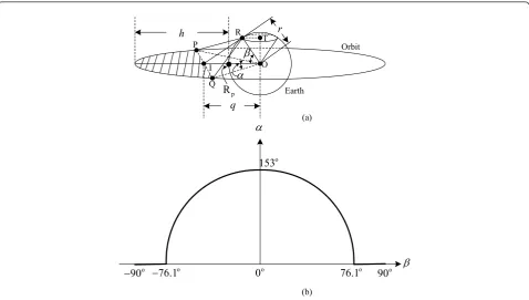
which together with linePQencloses the shadowed part of Figure 5a. In Figure 5a, the planeRPQis the tangent plane to the earth surface passing through R; PQis the intersection between the tangent plane RPQ and the orbital plane; OI⊥ PQ at pointI;Rpis the intersection between OI and the earth surface, which is the point intersecting the orbital plane of SV and the shortest arc along the earth surface fromRto the orbital plane;qis the shortest distance from the origin O to PQ; ais the angle∠POQ, corresponding to the visible arc PQ# andb is the elevation angle,∠ROI. From Figure 5a, we have
cosβ = r
Thus, the anglea can be expressed as a function of the elevation anglebas
α = 2 cos−1 receiver lies in the orbital plane of SV; while a = 0o occurs when |b|≥ 76.1o, i.e. when the receiver cannot see SV on the orbit. It can also be shown that the aver-age value ofais 137owhich occurs whenb= ± 49o.
Endnotes a
defined as the SV which in the frequency domain are close to “X” and can possibly collide with “X”. gThis representation denotes p1 (collision|1 visible) = 24.3% when the OBI is equal to 1 ms and p1 (collision|1 visi-ble) = 1.42% when the OBI is equal to 20 ms. For con-venience, we use this representation throughout this article.
Acknowledgements
This work is supported by the Alberta Informatics Circle of Research Excellence (iCORE), the Natural Sciences and Engineering Research Council of Canada (NSERC),