R E S E A R C H
Open Access
Comparative evaluation of ARIMA and ANFIS for
modeling of wireless network traffic time series
Rajnish K Yadav and Manoj Balakrishnan
*Abstract
Network traffic modeling significantly affects various considerations in networking, including network resource allocation, quality of service provisioning, network traffic management, congestion control, and bandwidth efficiency. These are very important issues in network protocol design, too. In this paper, a comprehensive comparison of modeling approaches of adaptive neuro fuzzy inference system (ANFIS) and autoregressive integrated moving average (ARIMA) for modeling of wireless network traffic in terms of typical statistical indicator and computational complexity has been attempted. ARIMA has been widely used in this area for past many years. On the other hand, ANFIS is comparatively new, and no network traffic modeling using ANFIS was attempted until recently to the best of our knowledge. At the same time, a detailed comparative performance evaluation of ANFIS with other modeling approaches in traffic modeling could not be found in existing literature. Reportedly, ANFIS provides a good precision in prediction in terms of statistical indicators and also gives effective description of network conditions at different times. However, the computational complexity of ANFIS for traffic modeling is a major concern and deserves a closer inspection. In our case of wireless network traffic, as a final result, we find that ANFIS model performs better than the best ARIMA model in three different scenarios.
Keywords:ARIMA; ANFIS; Network traffic modeling
1 Introduction
Network traffic modeling plays an important role in many areas of computer networks including but not lim-ited to network traffic management, quality of service (QoS) provisioning, network protocol design, and band-width allocation. This has led to a great interest among researchers in accurate modeling of network traffic. Ini-tial attempts in the past were mainly concentrated on Poisson modelingwhich did not compare well to the actual observations made at that time [1]. Then, a groundbreak-ing work by Leland et al. [2] proved that the network traffic exhibits self similarity and therefore its nature is entirely different, justifying not so accurate results from the Pois-son models. This seminal paper also laid the foundation for subsequent network traffic modeling attempts.
Many different modeling approaches have been tried since then to accurately model and capture this self-similar nature of network traffic. One important category of the type of models is statistical (or regressive) models,
which include autoregressive (AR), autoregressive moving average (ARMA), generalized autoregressive moving aver-age (GARMA), autoregressive integrated moving averaver-age (ARIMA), and fractional autoregressive integrated moving average (FARIMA) [3]. Another approach is that of frac-tional Gaussian noise (fGn) and fracfrac-tional Brownian mo-tion (fBn) which generally result in better accuracy as
compared to regressive models for long-range dependent
data [4]. Artificial neural network and fuzzy logic-based methods have also gathered significant attention [5-8]. Some authors have used modeling approaches based on least-mean kurtosis [9] and chaos theory [10].
ARIMA is a widely used statistical model for time series analysis and has also been used successfully in network traffic modeling [11,12]. Adaptive neuro fuzzy inference system (ANFIS) model [13] has been applied to forecast Internet traffic time series in [14]. Although other soft computing approaches have been tried earlier, ANFIS was not attempted prior to [14] in our know-ledge. ANFIS is a combination of fuzzy logic and neural network approaches and inherently carries the advan-tages of both. This makes ANFIS quite attractive option
* Correspondence:[email protected]
Department of Avionics, Indian Institute of Space Science and Technology (IIST), Trivandrum 695547, India
for this purpose. However, one major drawback of ANFIS is that it is computationally expensive and com-plex. This paper is an attempt to compare the modeling approaches of ARIMA and ANFIS under different sce-narios in order to conclude about their comparative suit-ability for computer network traffic modeling.
The paper has been organized as follows. In Section 2, we briefly highlight the related work in this area. Section 3 of this paper provides necessary description of ARIMA and ANFIS. Section 4 contains description of network traf-fic data collection and then data pre-processing. Modeling results and discussion have been presented in Section 5. Section 6 contains conclusions.
2 Related work
ARIMA has been discussed in [11,12] highlighting its use in modeling and prediction of network traffic. Authors in [4] discuss ARIMA modeling of traffic in an institutional wireless network. A good discussion on the application of ANFIS to forecast Internet traffic time series can be found in [14]. ANFIS method is compared with ARIMA in [15] for forecasting WiMAX traffic time series. The authors of [15] argue that ARIMA is better than ANFIS based on their comparison result which showed lower root mean square error (RMSE) and processing time for ARIMA. However in doing so, no proper reason was given for choosing a particular ARIMA model for comparison.
Figure 1Basic framework of FIS.
Weather forecasting is another prominent area in which attempts have been made to compare ARIMA and ANFIS approaches. The results of these comparisons, however, are contrasting. Some authors have found ARIMA preferable over ANFIS [16] while others recommend that ANFIS is a better approach [17]. We must note here that these are very specific applications in which dataset varies drastically from case to case leading to different results. In [18], com-parisons between the two approaches have been made to forecast electrical energy consumption wherein authors conclude that ANFIS is more appropriate than ARIMA.
3 Modeling approaches: ARIMA and ANFIS
We now describe the basic framework of modeling ap-proaches of ARIMA and ANFIS.
3.1 Autoregressive integrated moving average
In the framework of regression models, the computation of present output is done as a linear combination of some pre-specified number of past outputs and moving average of random white Gaussian noise [3].
Let us denote Ω as the lag operator such that ΩX
(t) =X(t−1). In general we writeΩτX(t) =X(t−τ). Also let us denoteΔas the difference operator so thatΔX(t) =X (t)−X(t−1). It can be observed thatΔτX(t) = (1−Ω)τX(t).
Let us also define two polynomial functions ϕ(Ω) = (1− ϕ1Ω−...−ϕmΩm) andθ(Ω) = (1−θ1Ω−...−θnΩn) where
ϕ1,ϕ2,....ϕn and θ1,θ2,....θn are coefficients of the lag
operator Ω; m and n are the degree of the polynomials,
respectively.
Given these notations, the definition of regressive models follows next.
An autoregressive model of orderm,generally denoted
by AR (m) [3] has the form
ϕð ÞΩ X tð Þ ¼εð Þt ð1Þ
whereε(t) is random white Gaussian noise.
An autoregressive moving average model of order (m,n), generally denoted by ARMA (m,n) [3] has the form
ϕð ÞΩ X tð Þ ¼θð ÞΩ εð Þt : ð2Þ
An autoregressive integrated moving average model of
order (m, τ, n) which is generally denoted by ARIMA
(m,τ,n) [3] has the form
ϕð ÞΩ ΔτX tð Þ ¼θð ÞΩεð Þt : ð3Þ
It can be seen that ARIMA is the most general of all the three regressive models discussed above. Although
Figure 3ANFIS architecture.
other more generalized regressive models are also avail-able, ARIMA will be the focus of our study in this paper.
3.2 Adaptive neuro fuzzy inference system
A fuzzy inference system (FIS) is a framework for com-putation based on the concepts of fuzzy set theory, fuzzy if then rules and fuzzy reasoning [13,19]. As shown in Figure 1, a FIS mainly has three conceptual components, viz., rule base, database, and reasoning mechanism. The rule base is a collection of fuzzy if-then rules which
decide the system’s behavior and response under
dif-ferent possible situations. The database contains the infor-mation about the membership functions in terms of their type and shape. Finally, the reasoning or decision-making mechanism is used to infer and derive output from the sys-tem. It may be noted that a FIS may need a fuzzification interface to convert crisp input values to fuzzy values suit-able for processing. However, when the inputs themselves are fuzzy then this may not be required. Similarly at the output side, a defuzzification interface is used because in almost all of the real-world application, we need a crisp output value.
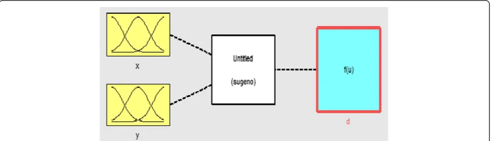
A neural network following the above discussed frame-work of a FIS results in ANFIS. For introductory pur-pose, a first-order Sugeno-type FIS(see [19]) in Figure 2 and equivalent ANFIS architecture in Figure 3 has been
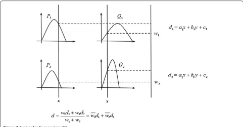
shown next. The following common rule set for first-order Sugeno fuzzy model can easily be verified:
Rule 1. IfxisP1andyisQ1, thend1=a1x+b1y+c1. Rule 2. IfxisP2andyisQ2, thend2=a2x+b2y+c2. In the ANFIS architecture shown in Figure 3, each node in the same layer has the similar function. Here we denote output of theith node in the layerlbyOli.
In layer 1, a linguistic label is associated with each input in terms of its membership grade. This membership grade can be defined by suitable membership functions μPið Þx
and μQ
ið Þx with appropriate parameters. The parameters associated with these membership functions are called premise or nonlinear parameters.
In layer 2, a Suitable T-norm operator (most commonly multiplication) is used to perform fuzzy AND operation of the input signals to get the output:
O2i ¼wi¼μPið Þx μQið Þx ; i¼1;2: ð4Þ
The output of this layer is often called the firing strength of the corresponding rule.
The ratio of a rule’s firing strength to the sum of
the firing strengths of all the rules is calculated in layer 3. This operation is also called normalization of firing strengths:
O3i ¼wi¼ wi w1þw2;
i¼1;2: ð5Þ
The output of layer 4 is given by
O4i ¼widi¼wiðaixþbiyþciÞ; i¼1;2: ð6Þ
Here,ai,bi, andci;i= 1, 2 are called consequent or
lin-ear parameters of ANFIS. The total number of parame-ters of ANFIS is the sum of premise and consequent parameters.
Table 1 Descriptive statistics of data samples and best fit model in three cases
Number of Samples
Min Max Mean Best fit model
Case 1 500 0.000 1.000 0.0986912 ARIMA (1,0,0)
Case 2 1,000 0.000 1.000 0.1074067 ARIMA (1,0,0)
Case 3 1,500 0.000 1.000 0.1084097 ARIMA (0,0,6)
Lastly in layer 5, the summation of incoming signals is performed to get the overall output of ANFIS.
O5i ¼ X
It must be noted that the structure of ANFIS explained above is not unique, and, in fact, arbitrary but meaning-ful assignment of node functions and configurations is possible.
A Sugeno-type FIS as in MATLAB Fuzzy Logic Tool-box is shown in Figure 4.
4 Network traffic collection and data pre-processing 4.1 Network traffic data collection
After completing a brief introduction of modeling ap-proaches of ARIMA and ANFIS, we now proceed to implement these concepts to the real-world network traffic data.
To begin, real-time network traffic trace is the first thing required. In the networking research community, Wireshark [20] is the most popular and sophisticated
network traffic monitoring tool. It can capture data packets from the network and provides important information like packet size, packet transfer rate, and packet capture time as well as data packet contents. We collected the packet statistics from an institutional wireless network, discarding the user data for this study. Matshark [21] was used to ex-tract the data from Wireshark and export it into MATLAB memory space.
4.2 Data pre-processing
The collected network traffic data was at nonuniform time scale. To get a time series data, samples at a uni-form time scale are required. Data samples were ex-tracted from the traffic trace at intervals of 0.1 s in MATLAB resulting in a time series data.
The data thus obtained was normalized using the operation:
normð Þ ¼x x−minð Þx
maxð Þx −minð Þx : ð8Þ
This ensured that all samples remain within the range [0, 1] so that the RMSE values after applying different models can be effectively compared.
Table 2 ANFIS specification for case 1
Specification Value
Selected ANFIS architecture 2-2-2-2
Number of nodes 55
Number of linear parameters 80
Number of nonlinear parameters 24
Total number of parameters 104
Number of training data pairs 500
Number of fuzzy rules 16
Figure 6RMSE curve of ANFIS model for case 2.
Table 3 ANFIS specification for case 2
Specification Value
Selected ANFIS architecture 2-2-2-2-2-2
Number of nodes 161
Number of linear parameters 448
Number of nonlinear parameters 48
Total number of parameters 496
Number of training data pairs 1,000
RMSE was used as a statistical indicator for assessing goodness of different models. The lower is the RMSE value, the better is the model. Mathematically, RMSE is given by
where ym and ^ym denote mth actual and model trained
data samples, respectively.Nis the sample size.
5 Results and discussion
We considered three different cases to evaluate and com-pare the performances of ARIMA and ANFIS. In the first case,N= 500 samples of the time series data were used for
modeling. In the second and third cases, N= 1,000 and
N= 1,500 samples were used respectively. Below we
de-scribe the individual cases using each approach.
5.1 ARIMA approach
IBM SPSS Statistics 17.0 [22] was used for ARIMA model-ing. SPSS is comprehensive and versatile tool for statistical analysis and it provides best fit ARIMA model for the
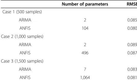
user-supplied data. The collected institutional network traffic data after necessary pre-processing was loaded into SPSS workspace. The best fit model was obtained with ARIMA (1,0,0) having RMSE of 0.085 for case 1, ARIMA (1,0,0) having RMSE of 0.089 for case 2, and ARIMA (0,0,6) having RMSE of 0.083 for case 3. The statistical description of data in three cases has been presented in Table 1 along with the best fit model in each case.
5.2 ANFIS approach
MATLAB Fuzzy Logic Toolbox [23] was used for ANFIS modeling. The following discussion details the results obtained under each case.
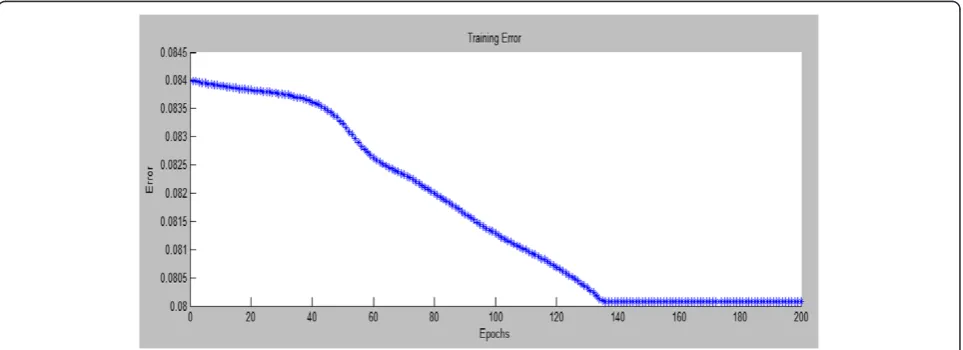
An RMSE of 0.080 was obtained with ANFIS model under case 1. Four past values of data were used as input, and the present value was used as output with each input having two membership functions (2-2-2-2 architecture). The variation of error with increasing epoch numbers is shown in Figure 5. It is observed that error continues to decrease till about 140 epochs and then it becomes almost constant. ANFIS specification for this case has been pre-sented in Table 2.
Figure 7RMSE curve of ANFIS model for case 3.
Table 4 ANFIS specification for case 3
Specification Value
Selected ANFIS architecture 2-2-3-2-3-2
Number of nodes 325
Number of linear parameters 1,008
Number of nonlinear parameters 56
Total number of parameters 1,064
Number of training data pairs 1,500
Number of fuzzy rules 144
Table 5 Summary of results
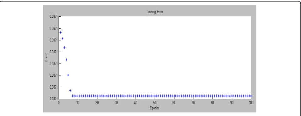
An RMSE of 0.087 was obtained with ANFIS model under case 2. Six past values of data were used as input, and the present value was used as output with each in-put having two membership functions (2-2-2-2-2-2 architecture). The variation of error with increasing epoch numbers is shown in Figure 6. It can be seen that error remains almost unchanged beyond seven epochs. ANFIS specification for this case has been presented in Table 3.
A careful reader might have observed that the error
along the Y-axis in Figure 6 remains almost equal to
0.0871 (shown only until four decimal places). This means that the error does not decrease appreciably with increasing epochs.
RMSE of 0.081 was obtained with ANFIS model under case 3. Six past values of data were used as input and present value as output with two inputs having three and rest others having two membership functions (2-2-3-2-3-2 architecture). The variation of error with increas-ing epoch numbers is shown in Figure 7. It is observed that the error curve is smooth contrary to earlier two cases and also that the error does not decrease appreciably with in-creasing epochs similar to case 2 above. ANFIS specifica-tion for this case has been presented in Table 4.
Noting that the number of parameters of ARIMA
(m, τ, n) is m+n+ 1, we summarize our results in
Table 5.
From Table 5, we see that ANFIS model results in lower RMSE as compared to ARIMA in all the three cases considered here. At the same time, it can also be observed that the number of parameters in ANFIS is much larger than ARIMA in each of these cases. Com-putational complexity is empirically related to the num-ber of parameters of a model which means that ANFIS is computationally more expensive and complex than ARIMA. The difference between the numbers of parame-ters becomes even larger when the number of inputs and the number of MFs of inputs of ANFIS are increased.
Hence, it is clear from the above results that although ANFIS performs better than ARIMA, this is achieved at the cost of complexity in computation which must be taken into consideration when ANFIS is used for net-work traffic modeling.
6 Conclusions
Network traffic modeling demands algorithms that are capable of dealing with the self-similar behavior of traf-fic data where conventional methods and assumptions fall short in terms of accuracy. Two different modeling approaches, autoregressive integrated moving average (ARIMA) and adaptive neuro fuzzy inference system (ANFIS), were applied to model the institutional network traffic data. For this study, three different cases are con-sidered for modeling with 500, 1,000, and 1,500 samples,
respectively, of an institutional wireless network traffic. We find that ANFIS performs better than ARIMA in all the three cases. However, this accuracy is achieved at the expense of computational complexity. Hence, it is recom-mended to use ANFIS approach only in those cases in which carrying out large computations is possible.
In future, coactive neuro fuzzy inference system (CANFIS) [19] can be used for network traffic modeling. Since it is a generalized form of ANFIS and allows avoid-ing some inherent constraints to ANFIS in its original form, we expect to get even better modeling results from CANFIS.
Competing interests
The authors declare that they have no competing interests.
Received: 7 August 2012 Accepted: 12 December 2013 Published: 22 January 2014
References
1. V Paxson, S Floyd, Wide-area traffic: the failure of Poisson modeling. IEEE/ACM Transac Network3, 226–244 (1995)
2. W Leland, M Taqqu, W Willinger, D Wilson, On the self-similar nature of Ethernet traffic (extended version). IEEE/ACM Transac Network2(1), 1–15 (1994) 3. M Ghaderi,On the relevance of self-similarity in network traffic prediction
(School of Computer Science, University of Waterloo, Waterloo, Canada). https://cs.uwaterloo.ca/research/tr/2003/28/TR-CS-2003-28.pdf. Accessed 23 July 2011
4. RK Yadav, Modeling of self similartraffic in wireless networks, inIEEE International Conference on High Performance Computing (HiPC) at Proceedings of Workshop on Next Generation Wireless Networks (WoNGeN) (Bangalore, 2011)
5. S Chabaa, A Zeroual, J Antari, Identification and prediction of internet traffic using artificial neural networks. J Intell Learning Syst Appl2(3), 147–155 (2010). 10.4236/jilsa.2010.23018
6. F Wang, H Xia, Network traffic prediction based on grey neural network integrated model, inInternational Conference on Computer Science and Software Engineering(Wuhan, 2008), pp. 915–918
7. N Piedra, J Chicaiza, J López, J García, Study of the application of neural networks in internet traffic engineering, inInformation Science and Computing (Institute of Information Theories and Applications, FOI ITHEA, 2008), pp. 3–47. ISSN: 1313–0455
8. A Rahman, P Kennedy, A Simmonds, J Edwards, Fuzzy logic based modelling and analysis of network traffic, in8th International Conference on Computer and Information Technology(Sydney, 2008), pp. 652–657 9. H Zhao, N Ansari, YQ Shi, Self-similar traffic prediction using least mean
kurtosis, inProceedings of International Conference on Information Technology: Coding and Computing Computers and Communications ITCC 2003 (Las Vegas, 2003), pp. 352–355
10. D Li, B Ji, H Xiang, The on-line prediction of self-similar traffic based on chaos theory, inInternational Conference on Wireless Communications, Networking and Mobile Computing, 2006. WiCOM 2006(Wuhan University, Wuhan, 2006), pp. 1–4
11. L Wang, Z Li, C Song, Network traffic prediction based on seasonal ARIMA model, in5th World Congress Intell Control Auto, vol. 2, (2004), pp. 1425–1428 12. B Zhou, D He, Z Sun, Traffic modeling and prediction using ARIMA/GARCH,
inModelling and Simulation Tools for Emerging Telecommunication Networks (Springer, New York, 2006), pp. 101–121
13. JSR Jang, ANFIS: adaptive- network based fuzzy inference system. IEEE Trans. Syst. Man and Cybernetics23(3), 665–685 (1993). 10.1109/21.256541 14. S Chabaa, J Antari, A Zeroual, ANFIS method for forecasting Internet
traffic time series, inMediterranean Microwave Symposium (MMS) (Tangiers, Morocco, 2009), pp. 1–4
15. CAS Hernandez, LFM Pedraza, OJP Salcedo, Comparative analysis of time series techniques ARIMA and ANFIS to forecast wimax traffic. Online J Electron Electric Eng (OJEEE)2(2), 223–228 (2010)
Conference on Informatics, Electronics and Vision (ICIEV)(Dhaka, 2013), pp. 1–6
17. M Tektas, Weather forecasting using ANFIS and ARIMA models. A case study for Istanbul. Environ Res Eng Manage1(51), 5–10 (2010)
18. R Yayar, M Hekim, V Yilmaz, F Bakirch, A comparison of ANFIS and ARIMA techniques in the forecasting of electrical energy consumption of Tokat province in Turkey. J Econ Social Stud1(2), 87–110 (2011)
19. JSR Jang, CT Sun, E Mizutani,Neuro-Fuzzy and soft computing: a computational approach to learning and machine intelligence(Prentice-Hall, Englewood Cliffs, 1997)
20. Wireshark. http://www.wireshark.org. Accessed 10 November 2011 21. Matshark. http://www.wireshark.org/lists/wireshark-users/201011/msg00028.
html. Accessed 14 November 2011
22. IBM SPSS Statistics. http://www-01.ibm.com/software/in/analytics/spss/ products/statistics. Accessed 20 November 2011
23. MATLAB Fuzzy Logic Toolbox. http://www.mathworks.in/products/fuzzy-logic. Accessed 25 November 2011
doi:10.1186/1687-1499-2014-15
Cite this article as:Yadav and Balakrishnan:Comparative evaluation of ARIMA and ANFIS for modeling of wireless network traffic time series.
EURASIP Journal on Wireless Communications and Networking20142014:15.
Submit your manuscript to a
journal and benefi t from:
7 Convenient online submission
7 Rigorous peer review
7 Immediate publication on acceptance
7 Open access: articles freely available online
7 High visibility within the fi eld
7 Retaining the copyright to your article