R E S E A R C H
Open Access
Fourth-order finite difference scheme and
efficient algorithm for nonlinear fractional
Schrödinger equations
Yan Chang
1and Huanzhen Chen
1**Correspondence:
1School of Mathematics and
Statistics, Shandong Normal University, Jinan, China
Abstract
To improve the computing efficiency, a fourth-order difference scheme is proposed and a fast algorithm is designed to simulate the nonlinear fractional Schrödinger (FNLS) equation oriented from the fractional quantum mechanics. The numerical analysis and experiments conducted in this article show that the proposed difference scheme has the optimal second-order and fourth-order convergence rates in time and space respectively, reduces its computation cost toO(MlogM), and recognizes accurately its physical feature of FNLS such as the mass balance.
Keywords: Fractional Schrödinger equation; Fourth-order difference scheme; Fast algorithm; Mass balance; Numerical analysis
1 Introduction
As is well known, numerous experiments have recognized that the fractional calculus can provide more flexible descriptions than the counterpart of integer-order for the real-world phenomena arising in various fields of science and engineering such as transmission of malaria disease [1], the constrained systems [2], the exothermic reactions model [3], and
the spring pendulum [4], which has attracted a mounting number of valuable research
work both mathematically and numerically during the last few years, see [5–16] and the references therein.
As one of the most significant applications of the fractional calculus in quantum me-chanics, the fractional Schrödinger equation (FNLS) was derived from the Lévy path in-tegrals instead of the Brownian path inin-tegrals as done in the classical Schrödinger
equa-tion given by Feynman and Hibbs [17]. The related mathematical analysis conducted in
the literature of FNLS proved the existence and uniqueness of ground state solution, the global solution, and the well-posedness of the solution to Cauchy problem, see [18,19]. For its computation, the implicitly conservative and split-step alternating direction differ-ence methods, Galerkin finite element method in one- or two-dimensional space, were proposed in [20–24], consecutively.
Checking carefully the existing numerical methods, we find that although the difference methods are easily implemented, they possess low computing accuracy, which motivates
us to design a high-order scheme to numerically solve the fractional Schrödinger. We also find that the nonlocality of the fractional Laplacian operator in FNLS often generates a non-sparse matrix of the discrete system, which makes the computation cost to beO(M2) if CG-like algorithms are used.
The goals of this article are as follows: (1) to adopt a fourth-order difference scheme by applying the Crank–Nicolson scheme to discrete the temporal derivative and truncating the weighted and shifted difference formula, [25] to discrete the fractional Laplacian op-erator; (2) to prove the solvability of the scheme and conduct numerical analysis to verify the convergence rates, as well as to show that the proposed numerical scheme can inherit the physical feature of FNLS such as the mass balance; (3) to design an efficient numerical algorithm through combining the Toeplitz structure of the coefficient matrix and the fast Fourier transform, which will reduce the computation cost fromO(M2) toO(MlogM); and (4) to conduct numerical experiments to verify the theoretical results and the physical properties.
The main novelties of this article at least are the following: (1) The scheme designed is a linearized one, due to which only a linear system needs to be solved, and thus the com-putational cost will be significantly reduced compared with the existing schemes; (2) The scheme possesses temporal convergence of second order and spatial convergence of fourth order, which, combining the fast stabilized bi-conjugate gradient (FSBiCG) algorithm, re-duces the computational cost greatly, and thus improves the computational efficiency.
The remainder of this article is arranged as follows. In Sect.2, we present the mathe-matical formula for FNLS and some related lemmas. In Sect.3, the fourth-order difference scheme is constructed. In Sect.4, we prove the solvability and convergence of the discrete system. The mass conservation properties as well as the stability are discussed in Sect.5. In Sect.6, a FSBiCG algorithm is proposed to reduce computation cost and storage. Several numerical experiments are reported to confirm our theoretical analysis in Sect.7.
Throughout the article we useCto denote a generic constant which may take different
values at different places.
2 Model problem and preliminaries
Consider the following fractional nonlinear Schrödinger equation (FNLS):
iut– (–)
α
2u+β|u|2u= 0, x∈(a,b),t∈[0,T], (2.1)
u(a,t) =u(b,t) = 0, t∈[0,T], (2.2)
u(x, 0) =u0(x), x∈[a,b]. (2.3)
Here,α∈(1, 2],i2= –1;u=u(x,t) is a complex-valued wave function describing the state of microscopic particles, which reflects the fluctuation of microscopic particles; the initial conditionu0(x) is a given smooth function vanishing at the end pointsx=aandx=b; the parameter β is a real constant describing the strength of the local interactions be-tween particles. FNLS is called focusing (attractive) or defocusing (repulsive), depending on whether the minus or plus sign appears in the front of the nonlinearity above, respec-tively. The Riesz fractional derivative (–)α2 is defined as
(–)α2u(x,t) = 1 2cosαπ2
–∞Dαxu(x,t) +xDα∞u(x,t)
in which–∞Dαxu(x,t) andxDα∞u(x,t) are expressed respectively by the following weighted
and shifted difference formula [25]:
–∞Dαxu(x,t) =hlim→0h–α
wherepis an integer, and
qk=
In fact,qkcan be expressed as the coefficients of the power series of the function (32– 2z+12z2)α,
In this paper, we adopt the ideas of [25] to truncate the Riesz fractional derivative (2.4). We first introduce several notations.
For positive integersMandN, we define a uniform partition forΩ= (a,b) byxj=a+jh, grid functionsu,w∈Vh, we define the discrete inner product and the associatedl2-norm as follows:
Collecting these notations introduced above, the fourth-order discretization for the fractional derivatives is given as follows.
Lemma 2.1([25]) Suppose thatα∈(1, 2),u∈L1(R),
–∞Dα+4x u,and its Fourier transform
(2.5)and(2.6)by
needs,λssatisfies the following system:
3 A fourth-order difference scheme
In this section, we adopt the Crank–Nicolson discretization in the temporal direction as well as the fourth-order difference discretization in the spatial direction to construct a difference scheme for FNLS (2.1).
Denotingun
j :=u(xj,tn) at the pointxjand at timetn, and noticing (2.4) as well as the
homogeneous boundary condition (2.2), we obtain
(–)α2un
Then we discrete FNLS (2.1) as follows:
iδtU
It is worth noting that (3.2) is not a self-starting scheme, and the numerical solution at
n= 1 should be provided by other schemes. For this, we introduce the following scheme
to seek forU1
For scheme (3.2)–(3.5b), only a linear system needs to be solved at each step.
4 Numerical analysis
metric positive definite matrix satisfying
αhU=KU, ∀U∈Vh. (4.2)
According to the spectral theorem [26], there is a real orthogonal matrixP and a real diagonal matrixD=diag(λ) satisfying
K=PDPT=PD12PTTPD12PT=LTL, (4.3)
whereD12 =diag(√λ) andL=PD12PT. It is easily shown that matrixLis a real symmetric positive definite matrix. Recalling the definition ofα
h, we obtain
αhU,V=h–αKU,V=h–α2LU,h–α2LV.
If we define the operatorΛαh by ΛαhU=h–α2LU, we could get (4.1). Thus, the proof is
completed.
Lemma 4.2 LetIm(·)andRe(·)stand for the imaginary part and the real part of a complex
number·,respectively.Then,for any grid function Un∈Vh, 0≤n≤N,we have
ImαhUn+21,Un+12= 0, (4.4)
ReαhUn+12,δtUn+12= 1
2τΛ
α hUn+1
2
–ΛαhUn2. (4.5)
Proof Lemma4.1implies (4.4) obviously. Using relation (4.1), we obtain
ReαhUn+12,δ tUn+
1
2
=ReΛαhUn+12,Λα hδtUn+
1
2
= 1
2τRe
ΛαhUn+1+ΛαhUn,ΛαhUn+1–ΛαhUn
= 1
2τΛ
α hUn+1
2
–ΛαhUn2, 0≤n≤N– 1. (4.6)
Thus, (4.5) is valid and the proof of the theorem is completed.
Lemma 4.3([27]) For any grid function Un∈Vh, 0≤n≤N,the inequality
Un2∞≤ 1 hU
n2
(4.7)
holds.
4.2 Solvability and convergence
In this subsection, we prove the solvability and convergence of difference scheme (3.2)– (3.5b) by induction.
Proof Noticing that difference scheme (3.2)–(3.5b) is a linear system, it suffices to prove that there exists a unique zero solution to its homogeneous system. For this purpose, we let the solutionUn= 0 forn= 0, (1), 1, . . . ,m– 1, and proveUm= 0 by induction.
Computing the discrete inner product of (4.8) withUmand then taking the real part yield
Um2+τ 2Im
αhUm,Um= 0. (4.9)
Using Lemma4.2, we obtain
Um= 0, (4.10)
which impliesUm= 0, and henceUmcan be solved uniquely. This completes the proof.
Before heading for the convergence analysis, we define the local truncation errorRn+
1
From (3.1) and Taylor’s expansion, we have
R(1)j ≤Cδ
Based on the truncation error introduced, the convergence results can be discussed. To start with, we define the error functionen∈V
hfor 0≤n≤Nas
ejn=unj –Ujn, 1≤j≤M– 1.
Theorem 4.5 Suppose that the original problem(2.1)–(2.3)has a smooth solution,and
Proof We prove this theorem by induction. Forn= 0, combining (2.3) with (3.3) implies the validity of (4.16).
Computing the discrete inner product of (4.17) withe(1)yields
i1 δ
e(1),e(1)h–hαe(1),e(1)h+βUj02e(1),e(1)h=R(1),e(1)h. (4.18)
Taking the imaginary part of (4.18), combining with the triangle inequalities and Cauchy inequalities, as well as Lemma4.2, we get
=β
Computing the discrete inner product of (4.23) withe12 and taking the imaginary part, using the triangle inequalities and Cauchy inequalities, noticing (4.4), (4.13), and (4.25), we obtain
whereCis a constant. Thus it holds that
e1≤Cδ+τ2+h4.
Again under the assumptionτ ≤Ch2as well asδ≤τ2, combining the above inequality
Since (4.16) is valid forn≤m– 1, we have
Gnj≤ |β|M0(M1+M0)
3enj+enj–1, 1≤j≤M– 1, 1≤n≤m– 1, (4.30)
which implies
Gn2≤C M0en
2
+en–12. (4.31)
Computing the discrete inner product of (4.28) withen+12 and taking the imaginary part, using the triangle inequalities andCauchyinequalities, noticing (4.4), (4.13), and (4.31), we have, for 1≤n≤m– 1,
en+12–en2
=τImGn+Rn+12,en+1+en
≤τen+12+en2+Gn2+Rn+122
≤τen+12+en2+CM0en 2
+en–12+ (b–a)CR
τ2+h42.
Whenτ≤12, we obtain
en+12–en2≤1 + 2(1 +CM0)τen 2
+ 2CM0τen–1 2
+ 2τ(b–a)CR
τ2+h42.
Using the above inequality, noticing (4.16), we get
em2≤2 + 2(1 +CM0)τem–1 2
+ 2CM0τem–2 2
+ 2τ(b–a)CR
τ2+h42
≤Cδ+τ2+h422 + 2(1 +CM0)τ+ 2CM0τ
+ 2τ(b–a)CR
τ2+h42
≤Cδ+τ2+h422 + 2τ+ 4CM0τ+ 2τ(b–a)
.
Letτ0:=2+4CM1
0+2(b–a), and chooseτsmall enough such thatτ≤τ0, then there is a constant
Csuch that
em2≤Cδ+τ2+h42, (4.32)
which immediately implies
em≤Cδ+τ2+h4.
Again under the assumptionτ≤Ch2as well asδ≤τ2, combining the above inequality with (4.7) gives
Um∞≤um∞+em∞≤M0+h– 1
2em≤M
0+Ch 7
and consequently, when 0 <h≤h0, we have
Um∞≤M0+ 1. (4.34)
This together with (3.5a)–(3.5b) implies (4.16) forn=m. By takingδ=τ2, it holds that
en ≤C(τ2+h4), i.e.,un–Un ≤C(τ2+h4). Thus the proof is completed by induction.
5 Mass conservation
In this section, we demonstrate that the discrete solution preserves the mass conservation, which further ensures the stability of the difference scheme proposed.
Theorem 5.1 Scheme(3.2)–(3.5b)preserves the mass in the following sense:
Qn=Q0, 0≤n≤N, (5.1)
where
Qn:=Un2 (5.2)
is the mass in the discrete sense.
Proof Computing the discrete inner product of (3.2) withUn+12, then taking the imaginary part, we obtain
Un+12=Un2, 0≤n≤N– 1, (5.3)
where (4.4) is used. This immediately implies (5.1).
Remark5.2 It follows from Theorem5.1that the numerical solution of (3.2)–(3.4) is long-time bounded, i.e., there exists some constantC> 0 such that
Un≤C, 0≤n≤N. (5.4)
Hence, scheme (3.2)–(3.5b) is unconditionallyL2-stable.
6 Fast stabilized bi-conjugate gradient algorithm (FSBiCG)
In this section, we develop a fast algorithm to numerically solve (3.2)–(3.5b). For conve-nience, we rewrite (3.2)–(3.5b) into the matrix form
(iI–δK+δβD0)U(1)=iU0, n=δ, (6.1a)
iI–τ
2K+
βτ
4 D1
U1=
iI+τ
2K–
βτ
4 D1
U0, (6.1b)
iI–τ
2K+
βτ
4 D2
Un+1=
iI+τ
2K–
βτ
4 D2
whereIis the unit matrix of size (M– 1)×(M– 1),Kis the discrete matrix of the fractional
It is easy to find thatKis a non-sparse Toeplitz matrix, which requiresO(M2) computa-tions andO(M2) storages while solving linear system (6.1a)–(6.1c) by the CG-like iteration method.
The aim for this section is to reduce the storage and calculation toO(M) andO(MlogM), respectively. For this, we shall combine the stabilized bi-conjugate gradient algorithm (SBiCG) with the Toeplitz structure of the coefficient matrices to construct the fast stabi-lized bi-conjugate gradient algorithm (FSBiCG) [28]. This needs the following three steps: The decomposition of a circulant matrix. It is known that a circulant matrix
CM–1can be diagonalized as follows [29,30]:
CM–1=FM–1–1diag(FM–1c)FM–1,
where c is the first column vector ofC,FM–1andFM–1–1are the discrete Fourier transform matrix and its inverse with entries given by
FM–1(j,l) =exp
It has been shown in [28] that the decomposition of circulant matrixCcould be carried out within a computational cost ofO(MlogM).
Computations for circulant matrix-vector multiplication. According to [30], a computational cost ofO(MlogM) and a memory ofO(M) are required while seek-ing for the circulant matrix-vector multiplication by FFT or iFFT.
Computations for Toeplitz matrix-vector multiplication. Notice that a (M–
1)×(M– 1) Toeplitz matrixTM–1is a matrix whose each descending diagonal from left to right is the same constantti,i= 0,±1, . . . ,±(M– 2), which needs storage ofO(M). On
with computational costO(MlogM). HereDM–1is a Toeplitz matrix whose each descend-ing diagonal from left to right isqi,i= 1, . . . ,M– 2, 0, 2 –M, . . . , –1.
Collecting these deductions above, we modify the traditional SBiCG to formulate our
fast SBiCG algorithm (FSBiCG), which is presented sentence by sentence in Algorithm1,
Algorithm 1The FSBiCG method for solvingAx=b
1: Given an initial guessX0and stopping toleranceε> 0
2: GivenC= (A(1, 1), . . . ,A(n, 1), 0,A(1,n), . . . ,A(1, 2))T
3: Compute:
4: x=FFT(C);X0= (X0; 0, . . . , 0)T
5: v=FFT(X0);y=v.∗x;z=iFFT(y);w=z(1 :n);r0=b–w
6: chooser0such that (r0,r0)= 0
7: p1=r0
8: fork= 1, 2 . . . do
9: pk= (pk; 0, . . . , 0)T
10: v=FFT(pk);y=v.∗x;z=iFFT(y);w1=z(1 :n)
11: αk= (rk–1,r0)/(w1,r0)
12: qk=rk–1–αkw1
13: qk= (qk; 0, . . . , 0)T
14: z=FFT(qk);w=z.∗x;μ=iFFT(z);w2=μ(1 :n)
15: ωk= (qk,w2)/(w2,w2)
16: x(k)=x(k–1)+α
kpk+ωkqk
17: rk=qk–ωkw2
18: ifrk2<εthen
19: stop
20: end if
21: βk=αk/ωk·(rk,r0)/(rk–1,r0)
22: pk=rk+βk(pk–ωkw1)
23: end for
Theorem 6.1 Compared with the SBiCG method,the FSBiCG algorithm proposed here reduces computational cost and storage fromO(M2)andO(M2)toO(MlogM)andO(M)
per iteration,respectively.
7 Numerical experiment
In this section, two numerical experiments are performed. In the first experiment, we pay particular attention to verifying the convergence rates and computation cost as well as the efficiency of the FBiCG compared with other algorithms. In the second experiment, we test the abilities of scheme (3.2)–(3.5b) to hold the physical characteristics-mass con-servation, subject to different initial values. These experiments are implemented by Mat-lab program on a family computer with configuration: Intel(R) Core(TM) i5-4590 CPU 3.3 GHz and 4 GB RAM.
7.1 Tests on the efficiency of the finite difference procedure and FSBiCG
Example7.1 Assume (a,b) = (0, 1),T= 1,β= 1, the analytic solution is prescribed to be
u(x,t) =x5(1 –x)5e–t (7.1)
subject to the initial condition
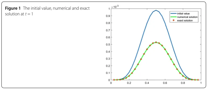
Figure 1The initial value, numerical and exact solution att= 1
and the right-hand source termf(x,t),
f(x,t) = – e –t
2cos(α 2π)
Γ(6)
Γ(6 –α)
x5–α+ (1 –x)5–α
– 5 Γ(7)
Γ(7 –α)
x6–α+ (1 –x)6–α+ 10 Γ(8)
Γ(8 –α)
x7–α+ (1 –x)7–α
– 10 Γ(9)
Γ(9 –α)
x8–α+ (1 –x)8–α+ 5 Γ(10)
Γ(10 –α)
x9–α+ (1 –x)9–α
– Γ(11)
Γ(11 –α)
x10–α+ (1 –x)10–α–ix5(1 –x)5e–t+x15(1 –x)15e–3t.
Hereα∈(1, 2).
Remark7.2 Considering the facts that the main aim of this numerical example is to
ver-ify the computing efficiency of FSBiCG, and the exact analytical solutions of (2.1) are
hardly available, we have to construct such an exact solution by attaching the nonzero source terms to the original systems without weakening the computing difficulties result-ing from the non-locality of the fractional operators. This equation may be thought of as a transformed version of the corresponding fractional Schrödinger equation (2.1) with non-homogeneous boundary conditions.
In this example, we calculate the convergence rates in space and time att= 1, and com-pare the computation time costs within different methods. Figure1depicts the initial con-dition, the numerical solution, and the exact solution withα= 1.9,h=216,τ =h2. From Fig.1, we find that the curve of numerical solution agrees well with the exact one. Letuh be the numerical solution. Tables1and2test the erroru–uhas well as the spatial and temporal convergence rates in theL2– and∞– sense with the time incrementτ =h2for
α= 1.3 andα= 1.9, respectively. The numerical results in Tables1and2show that the spatial and temporal convergence rates are 4 and 2 respectively, which is in accord with the theoretical expectations of Theorem4.5.
Table3tests the efficiency of the FSBiCG algorithm. We measure the time for the
com-plete simulation until t= 1 with the time incrementτ =h2 forα= 1.3 andα= 1.9. We
easily see that as the space stephbecomes smaller and smaller, the CPU time consumed
Table 1 Spatial convergence rates inL2and temporal rates
α 1/h 1/τ u–uhL2 Spatial rate Temporal rate
1.3 24 28 2.6919e-6
25 210 2.2419e-7 3.5858 1.7929
26 212 2.4566e-8 3.1899 1.5949
27 214 1.8398e-9 3.7390 1.8695
1.9 24 28 1.0250e-5
25 210 9.3139e-7 3.4601 1.7300
26 212 5.5518e-8 4.0683 2.0341
27 214 2.9951e-9 4.2122 2.1050
Table 2 Spatial convergence rates inL∞and temporal rates
α 1/h 1/τ u–uh∞ Spatial rate Temporal rate
1.3 24 28 6.8790e-6
25 210 3.9392e-7 4.1280 2.0640
26 212 5.4708e-8 2.8482 1.4241
27 214 4.2566e-9 3.6839 1.8733
1.9 24 28 1.5877e-5
25 210 1.5608e-6 3.3414 1.8357
26 212 1.1740e-7 3.7327 1.8663
27 214 6.9972e-9 4.0685 2.0342
Table 3 The CPU time consumed of the Gaussian elimination, the SBiCG method, and the FSBiCG method
α 1/h Gauss CPU (s) SBiCG CPU (s) Iter FSBiCG CPU (s) Iter
1.3 24 0.61 s 1.45 s 6 0.5277 s 8
25 4.95 s 14.05 s 7 2.5201 s 5
26 1 min 47 s 2 min 48 s 4 14.05 s 3
27 54 min 5 s 23 min 47 s 3 1 min 54 s 3
1.9 24 0.45 s 1.54 s 9 0.59 s 9
25 5.02 s 39.98 s 15 5.28 s 16
26 2 min 46 s 4 min 30 s 7 21.32 s 7
27 1h1 min 54 s 46 min 25 s 7 3 min 1 s 7
iterations are the same as SBiCG’s, which do not scale withM. For example, the CPU time of FSBiCG is 1 min 54 s compared to the SBiCG’s 23 min 47 s and the Gauss elimination’s 54 min 5 s ash=217,α= 1.3.
7.2 Tests on conservation of mass
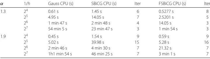
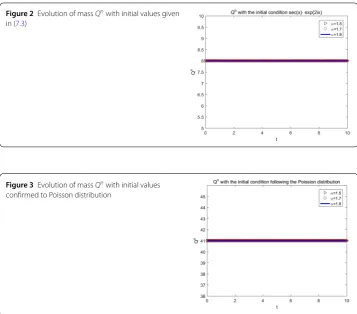
Example7.3 We takeβ= 1 andα= 1.5, 1.7, and 1.9, respectively, in (2.1) and select the step lengthsh= 0.25,τ =h2, the interval considered here is chosen to be [–20, 20]. The initial values are described in the following two categories to display the fitness of the numerical scheme for different systems. In the first category, the initial condition is chosen to be
u(x, 0) =sec(x)·exp(2ix), x∈[–20, 20], (7.3)
Figure 2Evolution of massQnwith initial values given in (7.3)
Figure 3Evolution of massQnwith initial values confirmed to Poisson distribution
The numerical results for the two initial values are presented in Figs.2–3, respectively. Figure2displays the mass subject to initial condition (7.3). To simulate the randomness of real quantum mechanics, we select the initial conditions as random sequences that obey the Poisson distribution and plot their mass in Fig.3. We can find that in Figs.2–3the curves of the mass are lines parallel to thet-axis, and we conclude that the mass is kept very well.
In addition, it deserves noting that the massQnis an intrinsic property of the material systems. Once the initial and boundary condition is given, mass is uniquely determined, which does not change with the parameterα, as is proven in Lemma5.1. As a result, the mass lines in Figs.2–3intercover.
8 Concluding remarks
We have established the well-defined fourth-order difference scheme for the nonlinear
fractional Schrödinger equation to approximate the unknown functionu. We found that
the highlights of our paper at least are as follows: (1) it improves the convergence rate compared with the existing method by developing a fourth-order difference scheme to-ward the fractional Riesz derivatives; (2) it proves the solvability of the scheme and the mass balance property inherited by the difference solution; (3) the fast algorithm can be designed to reduce the storage toO(M) and computational cost toO(MlogM).
Acknowledgements
This work is supported in part by the National Natural Science Foundation of China under Grant nos. 11471196, 10971254, 11471194.
Funding
National Natural Science Foundation of China under Grant nos. 11471196, 10971254, 11471194.
Availability of data and materials
Not applicable.
Competing interests
The authors declare that they have no competing interests.
Authors’ contributions
All authors contributed equally to this work. All authors read and approved the final manuscript.
Publisher’s Note
Springer Nature remains neutral with regard to jurisdictional claims in published maps and institutional affiliations.
Received: 25 May 2019 Accepted: 27 November 2019
References
1. Kumar, D., Singh, J., Al Qurashi, M., et al.: A new fractional SIRS-SI malaria disease model with application of vaccines, antimalarial drugs, and spraying. Adv. Differ. Equ.2019(1), 278 (2019)
2. Baleanu, D.: Fractional Hamiltonian analysis of irregular systems. Signal Process.86(10), 2632–2636 (2006) 3. Kumar, D., et al.: A new fractional exothermic reactions model having constant heat source in porous media with
power, exponential and Mittag-Leffler laws. Int. J. Heat Mass Transf.138, 1222–1227 (2019)
4. Baleanu, D., Asad, J.H., Jajarmi, A.: The fractional model of spring pendulum: new features within different kernels. Proc. Rom. Acad., Ser. A: Math. Phys. Tech. Sci. Inf. Sci.19(3), 447–454 (2018)
5. Baleanu, D., Rezapour, S., Mohammadi, H.: Some existence results on nonlinear fractional differential equations. Philos. Trans. R. Soc., Math. Phys. Eng. Sci.371(1990), 20120144 (2013)
6. Agarwal, R.P., Baleanu, D., Hedayati, V., Rezapour, S.: Two fractional derivative inclusion problems via integral boundary condition. Appl. Math. Comput.257, 205–212 (2015)
7. Baleanu, D., Asad, J.H., Jajarmi, A.: New aspects of the motion of a particle in a circular cavity. Proc. Rom. Acad., Ser. A: Math. Phys. Tech. Sci. Inf. Sci.19, 361–367 (2018)
8. Mohammadi, F., Moradi, L., Baleanu, D., et al.: A hybrid functions numerical scheme for fractional optimal control problems: application to nonanalytic dynamic systems. J. Vib. Control24(21), 5030–5043 (2018)
9. Baleanu, D., Mousalou, A., Rezapour, S.: A new method for investigating approximate solutions of some fractional integro-differential equations involving the Caputo–Fabrizio derivative. Adv. Differ. Equ.2017(1), 51 (2017) 10. Baleanu, D., Mousalou, A., Rezapour, S.: On the existence of solutions for some infinite coefficient-symmetric
Caputo–Fabrizio fractional integro-differential equations. Bound. Value Probl.2017(1), 145 (2017)
11. Baleanu, D., Mousalou, A., Rezapour, S.: The extended fractional Caputo–Fabrizio derivative of order 0≤σ< 1 on CR [0, 1]CR[0, 1] and the existence of solutions for two higher-order series-type differential equations. Adv. Differ. Equ.
2018(1), 255 (2018)
12. Kojabad, E.A., Rezapour, S.: Approximate solutions of a sum-type fractional integro-differential equation by using Chebyshev and Legendre polynomials. Adv. Differ. Equ.2017(1), 351 (2017)
13. Aydogan, S.M., Baleanu, D., Mousalou, A., et al.: On approximate solutions for two higher-order Caputo–Fabrizio fractional integro-differential equations. Adv. Differ. Equ.2017(1), 221 (2017)
14. Aydogan, M.S., Baleanu, D., Mousalou, A., Rezapour, S.: On high order fractional integro-differential equations including the Caputo–Fabrizio derivative. Bound. Value Probl.2018(1), 90 (2018)
15. Kumar, D., Singh, J., Purohit, S.D., et al.: A hybrid analytical algorithm for nonlinear fractional wave-like equations. Math. Model. Nat. Phenom.14(3), 304 (2019)
16. Bhatter, S., Mathur, A., Kumar, D., Singh, J.: A new analysis of fractional Drinfeld–Sokolov–Wilson model with exponential memory. Phys. A, Stat. Mech. Appl.2019,122578 (2019)
17. Laskin, N.: Fractional quantum mechanics. Phys. Rev. E, Stat. Phys. Plasmas Fluids Relat. Interdiscip. Topics62(3), 3135 (2000)
18. Feng, B.: Ground states for the fractional Schrödinger equation. Electron. J. Differ. Equ.2013, 127 (2013) 19. Hu, J., Jie, X., Hong, L.: The global solution for a class of systems of fractional nonlinear Schrödinger equations with
periodic boundary condition. Comput. Math. Appl.62(3), 1510–1521 (2011)
20. Wang, D., Xiao, A., Yang, W.: Crank–Nicolson difference scheme for the coupled nonlinear Schrödinger equations with the Riesz space fractional derivative. J. Comput. Phys.242(242), 670–681 (2013)
21. Wang, D., Xiao, A., Wei, Y.: A linearly implicit conservative difference scheme for the space fractional coupled nonlinear Schrödinger equations. J. Comput. Phys.272(3), 644–655 (2014)
22. Pengde, W., Huang, C.: An energy conservative difference scheme for the nonlinear fractional Schrödinger equations. J. Comput. Phys.293(3), 238–251 (2015)
23. Li, M., Huang, C., Wang, P.: Galerkin finite element method for nonlinear fractional Schrödinger equations. Numer. Algorithms74(2), 1–27 (2016)
24. Wang, P., Huang, C.: Split-Step Alternating Direction Implicit Difference Scheme for the Fractional Schrödinger Equation in Two Dimensions. Pergamon, Elmsford (2016)
26. Shubin, M.A.: Pseudodifferential Operators and Spectral Theory. Springer, Berlin (2001)
27. Xie, S.S., Li, G.X., Yi, S.: Compact finite difference schemes with high accuracy for one-dimensional nonlinear Schrödinger equation. Comput. Methods Appl. Mech. Eng.198(9), 1052–1060 (2009)
28. Wang, F., Chen, H., Wang, H.: Finite element simulation and efficient algorithm for fractional Cahn–Hilliard equation. J. Comput. Appl. Math.356, 248–266 (2019)
29. Davis, P.J.: Circulant Matrices. Am. Math. Soc., Providence (2013) 30. Gray, R.M.: Toeplitz and Circulant Matrices: a Review (2005)
31. Hajipour, M., Jajarmi, A., Baleanu, D.: On the accurate discretization of a highly nonlinear boundary value problem. Numer. Algorithms79(3), 679–695 (2018)