A numerical algorithm based on modified extended B spline functions for solving time fractional diffusion wave equation involving reaction and damping terms

(1)

R E S E A R C H

Open Access

A numerical algorithm based on modiﬁed

extended B-spline functions for solving

time-fractional diffusion wave equation

involving reaction and damping terms

Nauman Khalid

1

_{, Muhammad Abbas}

2*

_{, Muhammad Kashif Iqbal}

3

_{and Dumitru Baleanu}

4

*_{Correspondence:}

[email protected] 2_{Department of Mathematics,}

University of Sargodha, Sargodha, Pakistan

Full list of author information is available at the end of the article

Abstract

In this study, we have proposed an efficient numerical algorithm based on third degree modified extended B-spline (EBS) functions for solving time-fractional diffusion wave equation with reaction and damping terms. The Caputo

time-fractional derivative has been approximated by means of usual finite difference scheme and the modified EBS functions are used for spatial discretization. The stability analysis and derivation of theoretical convergence validates the authenticity and effectiveness of the proposed algorithm. The numerical experiments show that the computational outcomes are in line with the theoretical expectations. Moreover, the numerical results are proved to be better than other methods on the topic.

Keywords: Time-fractional diffusion wave equation; Finite difference formulation; Caputo’s time-fractional derivative; Modified extended B-spline functions; Modified B-spline collocation method

1 Introduction

The study of fractional calculus is considered to be an extension of classical calculus which has been given significant attentions in last couple of decades. Many applications of fractional differential equations are found in electro-chemistry, biomedical engineering, hydrology, probability theory and finance [1–6]. Fractional-order differential equations appear in mathematical modeling of several natural phenomena such as diffusion proce-dures, viscoelasticity, thermo-elasticity, seepage of a liquid, dynamical processes in self-similar and porous structures, wave propagation, anomalous diffusion transport, signal processing, control theory of dynamical systems, rheology and optics [7–11]. The time-fractional diffusion-wave equation (DWE) is one of them. This mathematical model is formulated from the classical DWE after replacing the second order time derivative by fractional derivative of orderα(1 <α≤2). Consider the following time-fractional DWE with Caputo’s fractional derivative involving reaction and damping terms:

∂αu(z,t) ∂tα +β

∂u(z,t)

∂t +γu(z,t) –

∂2u(z,t)

∂z2 =f(z,t), t∈[0,T],z∈[a,b], (1)

(2)

controlled by the following constraints:

u(z, 0) =φ0(z), ut(z, 0) =φ1(z); a≤z≤b, (2)

u(a,t) =ψ0(t), u(b,t) =ψ1(t); 0≤t≤T, (3) wheref(z,t),φi,ψi(i= 0, 1) are smooth functions with second order continuous

deriva-tives andβ,γare coeﬃcients of the reaction and damping terms, respectively. The Caputo fractional derivative ∂α

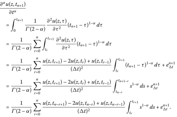
∂tαu(z,t) of orderα∈(1, 2] is deﬁned as ∂α

∂tαu(z,t) =

1 Γ(2 –α)

t

0

∂2u(z,τ) ∂τ2 (t–τ)

1–α

dτ, 1 <α≤2, (4)

whereΓ denotes the gamma function.

The study of exact and approximate solutions of differential/integral equations has al-ways remained an attractive area of research. The existence and behavior of unique solu-tions for some fractional-order quadratic Volterra equasolu-tions and nonlinear integral equa-tions has been discussed in [12–16]. In the last couple of decades many researchers studied the approximate solution of fractional-order DWE. Dinget al.[17] presented two numer-ical algorithms based on usual finite difference formulation for solving time-fractional DWE. Bhrawyet al.[18] employed the spectral tau method composed with the shifted Jacobi matrix for numerical treatment of second order fractional DWE. A numerical al-gorithm based on radial basis functions for solving fractional DWE was developed by Avazzadehet al.[19]. A triangular function algorithm based on the operational matrix of a fractional-order integration was discussed by Ebadianet al.[20] for solving a time-fractional DWE. Osamaet al. [21] employed the Sinc-Legendre collocation method to explore the numerical solution of a time-fractional DWE by reducing the problem into system of linear algebraic equations. Hooshmandasl et al.[22] numerically solved the fractional sub-diffusion and time-fractional DWE by employing the Galerkin technique depending on the fractional-order Legendre functions.

Chatterjeeet al.[23] used Bernstein polynomials to approximate truncated series for nonlinear fractional-order DWE. A numerical algorithm based on Chebyshev wavelets was formulated by Zhou and Xu [24] to obtain the approximate solution for time-fractional DWE. Numerous researchers have developed various methods for solving a time-fractional DWE; see [14, 25–27]. Recently, Kanwal et al. [28] presented a Ritz– Galerkin method together with two-dimensional Genocchi polynomials to establish the numerical solutions of a time-fractional DWE and a time-fractional Klein–Gordon equa-tion.

(3)

[32] discretized the spatial derivatives using extended cubic B-spline (ECBS) functions for solving a time-fractional advection–diﬀusion equation (ADE).

In the present paper, the application of modified ECBS functions has been presented for a numerical treatment of a time-fractional DWE involving reaction and damping terms. For temporal discretization, a usual finite difference approach consorted with Caputo’s time-fractional derivative has been used, while spatial derivatives are described by modi-fied ECBS functions.

The section-wise organization of the paper is as follows: In Sect.2, derivation of space derivatives via modiﬁed ECBS functions has been discussed. The temporal discretization is explained in Sect.3. The description of numerical method is presented in Sect.4. The stability and convergence analysis of the proposed scheme is given in Sect.5. To corrobo-rate the eﬃciency and validity of the present approach, the experimental results and com-parisons are displayed in Sect.6. Finally, concluding remarks are presented in Sect.7.

2 Modiﬁed extended cubic B-spline functions

Consider a partitiona=z0<z1<· · ·<zN=bof the interval [a,b] into subintervals [zi–1,zi]

with equal spacingh= 1

N(b–a),i= 1 : 1 :N.

whereαn_i(t) are time dependent constants, to be determined, and the ECBS blending func-tions of degree 4,ηi(z), are deﬁned as [32,36]

In the above formulation,μis a free parameter which is used to change the shape of the B-spline curve and –m(m– 2)≤μ≤1,mis the degree of ECBS [35]. Forμ= 0, the ECBS functions reduce to ordinary cubic B-spline functions. Further,η–1,η0, . . . ,ηN+1are taken in such a way that it forms spline basis over [a,b]. The values of ECBS functions and their derivative at nodal points are displayed in Table1. The approximate solutionU_in=U(zi,tn₎

with its ﬁrst and second derivative in terms of the time parameterαican be expressed as

(4)

Table 1 The coeﬃcients of ECBSηi(z) and their derivatives at nodezi

In the present study, the ECBS functions are modiﬁed in such a way that they pre-serve the diagonal dominance property. The modiﬁcation in ECBS functions is as follows [37]:

The second order diﬀerential operator approximation in time direction, using a ﬁnite dif-ference scheme, is given by

(5)

Hence

∂α_u₍_z_,_tn

+1) ∂tα =

1 Γ(3 –α)

n

r=0

br

u(z,tn–r+1) – 2u(z,tn–r) +u(z,tn–r–1)

(t)α +e

n+1

t , (10)

wherebr= (r+ 1)2–α_{– (}_r₎2–α_,_s₌_tn

+1–τ and the truncation errorent+1is bounded such

that

en_t+1≤σ(t)2, (11)

whereσ is a constant.

Lemma 3.1 The following properties are fulﬁlled by the coeﬃcients br[34]:

• br> 0andb0= 1,r= 1 : 1 :n,

• b0>b1>b2>· · ·>br,br→0asr→ ∞,

• –br+ (2br–br–1) + n–1

r=1(–br–1+ 2br–br+1) + (2b0–b1) = 1.

Using Eq. (10) in Eq. (1), we get the following form:

n

r=0

br

u(z,tn–r+1) – 2u(z,tn–r) +u(z,tn–r–1) Γ(3 –α)(t)α +β

u(z,tn+1) –u(z,tn)

t

+γu(z,tn+1) –

∂2_u₍_z_,_tn +1)

∂z2 =f(z,tn+1). (12)

Assumingρ=_Γ_(3–_α1₎₍_t₎α,β0=_tβ,un+1=u(z,tn+1), the above expression takes the follow-ing form:

(ρ+β0+γ)un+1– (2ρ+β0)un+ρun–1+ρ

n

r=1

brun–r+1– 2un–r+un–r–1

–∂ 2_un+1

∂z2 =f(z,tn+1), (13)

wheren= 0 : 1 :M. We use the initial condition to eliminateu–1_{, which will occur for}_n_{= 0,} i.e.

u–1=u1– 2tφ1(z). (14)

In particular, takingn= 0, the scheme takes the following form:

(ρ+β0+γ)u1– (2ρ+β0)u0+ρu–1= ∂2_u1

∂z2 +f(z,t1).

Using Eq. (14), the above equation simply leads to the following form:

(2ρ+β0+γ)u1– (2ρ+β0)u0= ∂2u1

(6)

4 Description of the numerical scheme

Using the ECBS approximations given in Eq. (7) in Eq. (13), the implicit ﬁnite diﬀerence formulation yields the following recurrence relation:

procedure. Making use of the initial conditions, we have

U_i0=φ0(zi), fori= 0 : 1 :N. (18)

In matrix notation, the above tri-diagonal system is expressed as

⎛

This section is for the discussion of the stability analysis and theoretical convergence of the proposed scheme.

5.1 Stability analysis

(7)

presented numerical algorithm for solving time-fractional DWE. Let Φ_inbe the growth factor of the fourier mode andΦ˜_inbe its approximation. Deﬁne the error term_inas

n_i =Φ_in–Φ˜_in, i= 1 : 1 :N– 1,n= 0 : 1 :M, (20) andn_{= [}n

1,2n,·,Nn–1]T.

It is suﬃcient to analyze stability of the scheme presented in Eq. (16) for force-free case (f = 0) only. The round-oﬀ error equation has been obtained from Eqs. (20) and (16) as

The initial/boundary conditions are satisﬁed by the error equation such as

0_i =φ0(zi), (t)0i =φ1(zi), i= 1 : 1 :N, (22)

and

n₀=ψ0(tn), Nn =ψ1(tn), n= 0 : 1 :M. (23)

Now, we deﬁne the mesh function as follows:

n=

Expressingn(z) in the Fourier series form:

n(z) =

Using the norm deﬁnition, we have

(8)

Using the Parseval equality,_ab|n_|2_dz₌∞

Suppose the solution in the Fourier series form is presented as follows:

n_j =ξneiλjh, (28)

Proof We prove this result by induction. Forn= 0, Eq. (30) implies

Theorem 1 The implicit collocation scheme(16)is unconditionally stable.

Proof By making use of Eq. (27) and Lemma5.1, we get

n

2≤ 0

(9)

From the aforementioned relations we conclude that the proposed scheme (16) is

uncon-ditionally stable.

5.2 Convergence analysis

We follow Kadalbajoo and Arora [39] to examine the convergence of the proposed scheme. First of all, we state a theorem due to Boor [40] and Hall [41] which plays a key role for the convergence analysis of the proposed scheme.

Theorem 2 Let,u(z,t)belongs to C4_[_a_,_b_],_{f belongs to C}2_[_a_,_b_]_and_Π₌_{_a₌_z

0,z1, . . . ,zN=

b}be a partition such that zi=ih,i= 1 : 1 :N.LetU˜(z,t)denote the unique spline approx-imation to the present problem at the knots z∈Π,then∀t≥0,∃aj,free of h,s.t.

Dju(z,t) –U˜(z,t) _∞≤ajh4–j, j= 0, 1, 2. (31)

Lemma 5.2 The modiﬁed ECBS set{η0,η1, . . . ,ηN}presented in Eq. (8)satisfy the inequal-ity,

N

i=0

ηi(z)≤

7

4. (32)

Proof Using the triangular inequality, we have

N

i=0 ηi(z)

≤

N

i=0 η_i(z).

For any nodal pointzi, we get

N

i=0

η_i(z)=ηi–1(zi)+ηi(zi)+ηi+1(zi)

=4 –μ 24 +

8 +μ 12 +

4 –μ 24 = 1 <

7 4.

Furthermore, for a pointz∈[zi,zi+1], we obtain

N

i=0

η_i(z)=ηi–1(z)+ηi(z)+ηi+1(z)+ηi+2(z)= 20 +μ

12 ,

where

ηi–1(z)≤ 4 –μ

24 , ηi(z)≤ 8 +μ

12 , ηi+1(z)≤ 8 +μ

12 , ηi+2(z)≤ 4 –μ

24 .

Since –8≤μ≤1, we have 1≤20+₁₂μ≤7 4. Hence,

N

i=0

ηi(z)≤

7

(10)

Theorem 3 The numerical approximation U(z,t)to the closed form solution u(z,t)exists for the time-fractional problem(1)–(3).Also,if f∈C2_{[0, 1],}_{we have}

u(z,t) –U(z,t)_∞≤κh2, ∀t≥0 (33)

where h is suﬃciently small andκ> 0is,a constant,free of h.

Proof LetU˜(z,t) =_iN₌₀di(t)ηi(z) be the computed spline for the approximate solution U(z,t) and exact solutionu(z,t). Using the triangular inequality, the expression can be written as

u(z,t) –U(z,t)_∞≤u(z,t) –U˜(z,t)_∞+U˜(z,t) –U(z,t)_∞.

Using (31), we have

u(z,t) –U(z,t)_∞≤a0h4+U˜(z,t) –U(z,t)_∞. (34)

LetLu(zi,t) =LU(zi,t) =f(zi,t),i= 0 : 1 :N, be the collocation conditions, then

LU˜(z,t) =f˜(zi,t), i= 0 : 1 :N.

At any time leveln, the given problem in the form of the diﬀerence equationL(U˜(zi,t) – U(zi,t)) can be written as follows:

(ρ+β0+γ)c1–c4

ν_in_–1+1+(ρ+β0+γ)c2–c5

ν_in+1+(ρ+β0+γ)c1–c4

ν_in₊₁+1

= (2ρ+β0)

c1νni–1+c2νin+c1νin+1 –ρ

c1νin–1–1+c2νin–1+c1νin+1–1

–ρ

n

r=1

brc1

ν_in_–1–r+1– 2ν_in_–1–r+ν_in_–1–r–1 +c2

ν_in–r+1– 2ν_in–r+ν_in–r–1

+c1

νn_i₊₁–r+1– 2ν_in₊₁–r+ν_in₊₁–r–1 +f_in+1. (35)

Also, the boundary conditions take the following form:

c1νin–1+1+c2νin+1+c1νin+1+1= 0, i= 0,N,

where

ν_in=αn_i –dn_i, i= 0 : 1 :N,

and

Ω_in=h2f_in–f˜_in, i= 0, . . . ,N. It is evident from (31) that we have

Ωn

i=h2fin–f˜in≤ah4.

We deﬁneΩn₌_max_{|_Ωn

(11)

Forn= 0, Eq. (35) together with (14) takes the following form:

Using the initial condition,e0_{= 0, we have}

Taking absolute values ofΩ_inandν_inwith a suﬃciently small mesh sizeh, we have

˜

Taking the inﬁnite norm and using Lemma5.1, we obtain

(12)

From Eq. (38), Eq. (34) takes the following form:

u(z,t) –U(z,t)_∞≤a0h4+ 1.75ah2=κh2,

whereκ=a0h2+ 1.75a.

From the aforementioned theorem and Eq. (11) we conclude that the proposed numer-ical approach is convergent. Hence,

u(z,t) –U(z,t)_∞≤κh2+σ(t)2,

whereκandσ are constants.

6 Numerical examples

To examine the accuracy of the proposed computational scheme, some test examples are considered for the time-fractional DWE. TheL2andL∞norms are used to calculate the absolute errors of the proposed method as in [42]. We have

L2= _hN

i=0

U(zi,t) –u(zi,t)2, L∞= max

0≤i≤N

U(zi,t) –u(zi,t).

The experimental order of convergence (EOC) is calculated to be [43]

EOC =log(L∞(n)/L∞(2n)) log(2) .

The numerical results obtained from the modiﬁed ECBS method are compared with given exact solutions and the numerical methods available in the literature. The software pack-age MATHEMATICA 9.0 is used to run the simulation.

Example1 Consider the time-fractional DWE [33]

∂α_u₍_z_,_t₎

∂tα –

∂2u(z,t) ∂z2

=sin(πz)

2t2–α

Γ(3 –α)–

t1–α

Γ(2 –α)+π

2_t2_–_t _, _z_∈_[_a_,_b_],_t_∈_[0,_T_],

with the conditions

u(z, 0) = 0, ut(z, 0) = –sin(πz),

(13)

Table 2 Error normL_∞att= 0.2, 0≤z≤1 andα= 1.5 for Example1

150 0.00115 3.049×10

–6 _7.719_×₁₀–16

1 30

1

200 0.00021 3.035×10

–6 _8.826_×₁₀–16

1 40

1

200 0.00019 1.281×10

–6 _2.990_×₁₀–16

1 40

1

210 0.00006 1.280×10

–6 _2.225_×₁₀–16

1 45

1

220 0.00004 8.989×10

–7 _9.935_×₁₀–17

100 0.01064 3.113×10

–5 _4.080_×₁₀–14

1 30

1

200 0.00736 9.178×10

–6 _9.718_×₁₀–15

1 50

1

250 0.00653 1.982×10

–6 _3.602_×₁₀–15

1 50

1

300 0.00586 1.980×10

–6 _3.214_×₁₀–15

1 60

1

400 0.00494 1.149×10

–6 _2.169_×₁₀–15

1 60

1

450 0.00460 1.443×10

–6 _2.025_×₁₀–15

N CuTBSM [33] Present method

(14)

Figure 2Exact and approximate solutions for Example1, whenN= 32,α= 1.5 andt= 0.01

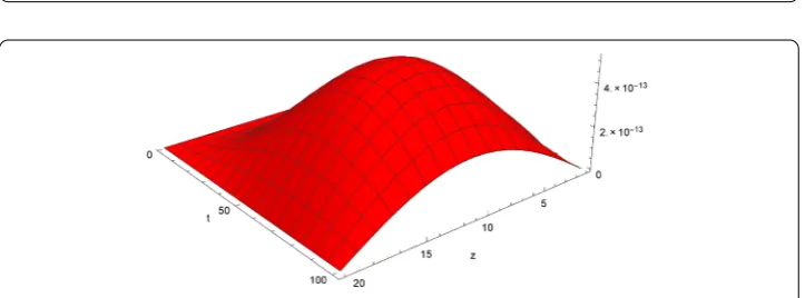
Figure 3Absolute error graph for Example1att= 1 whenN= 20,α= 1.3 and 0≤z≤1

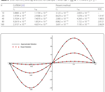
and CuTBSM [33]. Also the results elaborated in Table3show a far better agreement with the analytical exact solution than the other methods att= 0.4,α= 1.7 for diﬀerent choices ofhandt. The EOC is portrayed in Table4. The error normsL2andL∞are also compared with the method given in [33]. In Fig.1, the approximate solution at diﬀerent time levels is shown in one frame when –1≤z≤1. The three dimensional visuals given in Fig.2elucidate our claim about accuracy of the proposed scheme forN= 32,t= 0.01 andt= 2. The 3D absolute error graph is displayed in Fig.3forN= 20,t= 1,t= 0.01 andα= 1.3.

Example2 Consider the time-fractional DWE involving damping term [45]

∂αu(z,t) ∂tα +

∂u(z,t) ∂t –

∂2u(z,t) ∂z2 =

6t3–α

Γ(4 –α)+ 3t

2_–_t3 _ez_, _z_∈_{[0, 1],}_t_∈_[0,_T_],

with the initial/boundary conditions

u(z, 0) =ut(z, 0) = 0

and

u(0,t) =t3, u(1,t) =t2e.

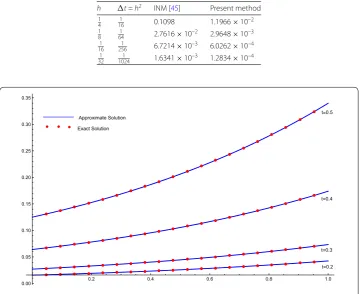
The analytical exact solution isu(z,t) =t3_ez_{. In Table}₅_{, the approximate results returned}

(15)

Table 5 Maximum absolute error (L_∞) whenα= 1.85 for Example2

h t=h2 INM [45] Present method 1

4 1

16 0.1098 1.1966×10–2 1

8 1

64 2.7616×10–2 2.9648×10–3 1

16 1

256 6.7214×10–3 6.0262×10–4 1

32 1

1024 1.6341×10

–3 _1.2834_×₁₀–4

Figure 4Exact and approximate solutions for Example2att= 0.2, 0.3, 0.4, 0.5 whenN= 10,α= 1.85 and t= 0.001

Figure 5Exact and approximate solutions for Example2, whenN= 50,α= 1.25,t= 2 andt= 0.01

forα= 1.85,t= 1 andt=h2_{. The graphical representation of exact and numerical} solu-tions at diﬀerent time levels is captured in Fig.4. Figure5depicts the physical behavior of exact and numerical solutions atN= 50,α= 1.25 andt= 1. The comparison of the results shows a reﬂexive behavior of the approximate solution to the analytical exact solution. Figure6shows a 3D absolute error graph forα= 1.5,t= 1,t= 0.01 andN= 16.

Example3 Consider a time-fractional DWE with a reaction term [19]

∂α_u₍_z_,_t₎

∂tα +u(z,t) –

∂2_u₍_z_,_t₎ ∂z2 =

2t2–α_sinh₍_z₎

(16)

Figure 6Absolute error graph for Example2att= 1 whenN= 16,α= 1.5 and 0≤z≤1

Table 6 Approximate results whenN= 50 att= 1 for Example3

z α= 1.25 α= 1.5

RBF [19] CuTBSM [33] Present RBF [19] CuTBSM [33] Present

0.1 6.63×10–4 _2.10_×₁₀–6 _4.29_×₁₀–9 _6.55_×₁₀–4 _2.08_×₁₀–6 _3.23_×₁₀–9 0.2 5.46×10–4 _4.07_×₁₀–6 _5.96_×₁₀–9 _5.33_×₁₀–4 _4.05_×₁₀–6 _4.49_×₁₀–9 0.3 5.07×10–4 _5.81_×₁₀–6 _7.06_×₁₀–9 _4.89_×₁₀–4 _5.79_×₁₀–6 _5.77_×₁₀–9 0.4 4.68×10–4 _7.20_×₁₀–6 _8.54_×₁₀–9 _4.48_×₁₀–4 _7.20_×₁₀–6 _7.90_×₁₀–9 0.5 4.56×10–4 _8.12_×₁₀–6 _9.02_×₁₀–9 _4.34_×₁₀–4 _8.08_×₁₀–6 _8.09_×₁₀–9 0.6 4.53×10–4 _8.41_×₁₀–6 _7.61_×₁₀–9 _4.32_×₁₀–4 _8.38_×₁₀–6 _7.28_×₁₀–9 0.7 4.75×10–4 _7.92_×₁₀–6 _7.09_×₁₀–9 _4.57_×₁₀–4 _7.90_×₁₀–6 _6.78_×₁₀–9 0.8 4.99×10–4 _6.49_×₁₀–6 _5.72_×₁₀–9 _4.85_×₁₀–4 _6.47_×₁₀–6 _4.70_×₁₀–9 0.9 5.90×10–4 _3.92_×₁₀–6 _3.82_×₁₀–9 _5.83_×₁₀–4 _3.91_×₁₀–6 _2.64_×₁₀–9

subject to the initial/boundary constraints

u(z, 0) =ut(z, 0) = 0,

u(0,t) = 0, u(1,t) =sinh(1)t2.

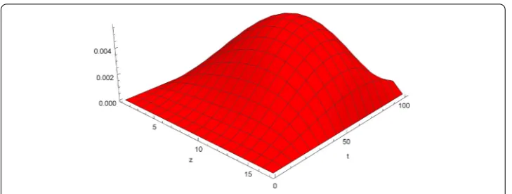
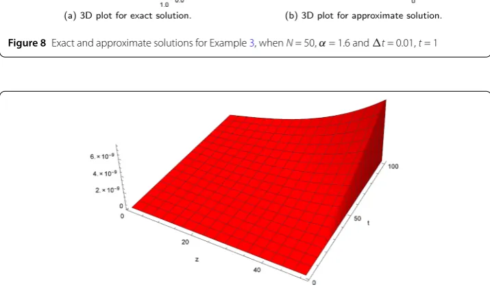
The exact solution isu(z,t) =t2sinh(z). In Table6, the numerical results obtained by means of the modiﬁed ECBS method are compared with the radial basis function (RBF) method introduced in [19] and CuTBSM developed in [33]. The absolute computational errors corresponding toN= 50,μ= –0.0196,α= 1.25 andα= 1.5 are reported in Table6. The numerical solutions obtained by the proposed numerical method at diﬀerent time levels are depicted in Fig.7. The 3D space-time graphs of exact and approximate solutions forN= 50,α= 1.6,t= 1 andt= 0.01 are displayed in Fig.8. The three dimensional pictorizations of the absolute error forN= 50,α= 1.5,t= 1 andt= 0.01 are given in Fig.9.

7 Conclusion

(17)

Figure 7Exact and approximate solutions for Example3att= 2, 4, 6, 8, 10 whenN= 10,α= 1.5 andt= 0.01

Figure 8Exact and approximate solutions for Example3, whenN= 50,α= 1.6 andt= 0.01,t= 1

(18)

convergence is of order 2. The computational outcomes are proved to be more reliable than the results found in RBF [19], CuTBSM [33], HF [44] and INM [45].

Acknowledgements

The authors are grateful to the anonymous reviewers for their helpful, valuable comments and suggestions in the improvement of this manuscript.

Funding Not applicable.

Availability of data and materials Not applicable.

Competing interests

The authors declare that they have no competing interests.

Authors’ contributions

All authors equally contributed to this work. All authors read and approved the ﬁnal manuscript.

Author details

1_{Department of Mathematics, National College of Business Administration & Economics, Lahore, Pakistan.}2_Department

of Mathematics, University of Sargodha, Sargodha, Pakistan. 3_{Department of Mathematics, Government College}

University, Faisalabad, Pakistan.4_{Department of Mathematics, Faculty of Arts and Sciences, Cankaya University, Ankara,}

Turkey.

Publisher’s Note

Springer Nature remains neutral with regard to jurisdictional claims in published maps and institutional aﬃliations.

Received: 15 May 2019 Accepted: 27 August 2019 References

1. Miller, K.S., Ross, B.: An Introduction to the Fractional Calculus and Fractional Differential Equations (1993) 2. Podlubny, I.: Fractional Differential Equations: An Introduction to Fractional Derivatives, Fractional Differential

Equations, to Methods of Their Solution and Some of Their Applications. Mathematics in Science and Engineering, vol. 198 (1998)

3. Mainardi, F.: Fractional Calculus, pp. 291–348 (1997)

4. Benson, D.A., Wheatcraft, S.W., Meerschaert, M.M.: Application of a fractional advection–dispersion equation. Water Resour. Res.36(6), 1403–1412 (2000)

5. Meerschaert, M.M., Tadjeran, C.: Finite diﬀerence approximations for fractional advection–dispersion ﬂow equations. J. Comput. Appl. Math.172(1), 65–77 (2004)

6. Meerschaert, M.M., Scalas, E.: Coupled continuous time random walks in ﬁnance. Phys. A, Stat. Mech. Appl.370(1), 114–118 (2006)

7. Koeller, R.: Applications of fractional calculus to the theory of viscoelasticity. J. Appl. Mech.51(2), 299–307 (1984) 8. Shivanian, E., Jafarabadi, A.: Applications of Fractional Calculus in Physics (2000)

9. Kilbas, A.A., Srivastava, H.M., Trujillo, J.J.: Theory and Applications of Fractional Diﬀerential Equations. Elsevier, Amsterdam (2006)

10. Aleroev, T., Aleroeva, H., Huang, J., Nie, N., Tang, Y., Zhang, S.: Features of seepage of a liquid to a chink in the cracked deformable layer. Int. J. Model. Simul. Sci. Comput.1(3), 333–347 (2010)

11. Machado, J.T., Kiryakova, V., Mainardi, F.: Recent history of fractional calculus. Commun. Nonlinear Sci. Numer. Simul. 16(3), 1140–1153 (2011)

12. Mishra, L.N., Sen, M.: On the concept of existence and local attractivity of solutions for some quadratic Volterra integral equation of fractional order. Appl. Math. Comput.285, 174–183 (2016)

13. Mishra, V.N.: Some problems on approximations of functions in Banach spaces. Ph.D. thesis (2007)

14. Mishra, V., Vishal, K., Das, S., Ong, S.H.: On the solution of the nonlinear fractional diﬀusion-wave equation with absorption: a homotopy approach. Z. Naturforsch. A69(3–4), 135–144 (2014)

15. Deepmala: A study on ﬁxed point theorems for nonlinear contractions and its applications. Ph.D. thesis (2014) 16. Esbo, M.R., Vazifeshenas, Y., Asboei, A.K., Mohammadyari, R., Vandana, V.: Numerical simulation of twisted tapes ﬁtted

in circular tube consisting of alternate axes and regularly spaced tapes. Acta Sci., Technol.40, e37348 (2018) 17. Ding, H., Li, C.: Numerical algorithms for the fractional diﬀusion-wave equation with reaction term. Abstr. Appl. Anal.

2013, Article ID 493406 (2013)

18. Bhrawy, A., Doha, E.H., Baleanu, D., Ezz-Eldien, S.S.: A spectral tau algorithm based on Jacobi operational matrix for numerical solution of time fractional diﬀusion-wave equations. J. Comput. Phys.293, 142–156 (2015)

19. Avazzadeh, Z., Hosseini, V., Chen, W.: Radial basis functions and FDM for solving fractional diﬀusion-wave equation. Iran. J. Sci. Technol., Sci.38(3), 205–212 (2014)

20. Ebadian, A., Fazli, H.R., Khajehnasiri, A.A.: Solution of nonlinear fractional diﬀusion-wave equation by traingular functions. SeMA J.72(1), 37–46 (2015)

(19)

22. Hooshmandasl, M., Heydari, M., Cattani, C.: Numerical solution of fractional sub-diﬀusion and time-fractional diﬀusion-wave equations via fractional-order Legendre functions. Eur. Phys. J. Plus131(8), 268 (2016) 23. Chatterjee, A., Basu, U., Mandal, B.: Numerical algorithm based on Bernstein polynomials for solving nonlinear

fractional diﬀusion-wave equation. Int. J. Adv. Appl. Math. Mech.5, 9–15 (2017)

24. Zhou, F., Xu, X.: Numerical solution of time-fractional diﬀusion-wave equations via Chebyshev wavelets collocation method. Adv. Math. Phys.2017, Article ID 2610804 (2017)

25. Mitkowski, W.: Approximation of fractional diﬀusion-wave equation. Acta Mech. Autom.5, 65–68 (2011) 26. Delic, A.: Fractional in time diﬀusion-wave equation and its numerical approximation. Filomat30(5), 1375–1385

(2016)

27. Ferreira, M., Vieira, N.: Fundamental solutions of the time fractional diﬀusion-wave and parabolic Dirac operators. J. Math. Anal. Appl.447(1), 329–353 (2017)

28. Kanwal, A., Phang, C., Iqbal, U.: Numerical solution of fractional diﬀusion wave equation and fractional Klein–Gordon equation via two-dimensional Genocchi polynomials with a Ritz–Galerkin method. Computation6(3), 40 (2018) 29. Khalid, N., Abbas, M., Iqbal, M.K.: Non-polynomial quintic spline for solving fourth-order fractional boundary value

problems involving product terms. Appl. Math. Comput.349, 393–407 (2019)

30. Amin, M., Abbas, M., Iqbal, M.K., Baleanu, D.: Non-polynomial quintic spline for numerical solution of fourth-order time fractional partial diﬀerential equations. Adv. Diﬀer. Equ.2019(1), 183 (2019)

31. Yaseen, M., Abbas, M.: An eﬃcient computational technique based on cubic trigonometric B-splines for time fractional Burgers’ equation. Int. J. Comput. Math. (2019).https://doi.org/10.1080/00207160.2019.1612053

32. Mohyud-Din, S.T., Akram, T., Abbas, M., Ismail, A.I., Ali, N.H.: A fully implicit finite difference scheme based on extended cubic B-splines for time fractional advection–diffusion equation. Adv. Differ. Equ.2018(1), 109 (2018)

33. Yaseen, M., Abbas, M., Nazir, T., Baleanu, D.: A finite difference scheme based on cubic trigonometric B-splines for a time fractional diffusion-wave equation. Adv. Differ. Equ.2017(1), 274 (2017)

34. Sayevand, K., Yazdani, A., Arjang, F.: Cubic B-spline collocation method and its application for anomalous fractional diﬀusion equations in transport dynamic systems. J. Vib. Control22(9), 2173–2186 (2016)

35. Shukla, H., Tamsir, M.: Extended modiﬁed cubic B-spline algorithm for nonlinear Fisher’s reaction–diﬀusion equation. Alex. Eng. J.55(3), 2871–2879 (2016)

36. Wasim, I., Abbas, M., Iqbal, M.K.: A new extended B-spline approximation technique for second order singular boundary value problems arising in physiology. J. Math. Comput. Sci.19(4), 258–267 (2019)

37. Mittal, R., Jain, R.: Numerical solutions of nonlinear Burgers’ equation with modiﬁed cubic B-splines collocation method. Appl. Math. Comput.218(15), 7839–7855 (2012)

38. Boyce, W.E., DiPrima, R.C., Meade, D.B.: Elementary Diﬀerential Equations and Boundary Value Problems, vol. 9 (1992) 39. Kadalbajoo, M.K., Arora, P.: B-spline collocation method for the singular-perturbation problem using artiﬁcial viscosity.

Comput. Math. Appl.57(4), 650–663 (2009)

40. de Boor, C.: On the convergence of odd-degree spline interpolation. J. Approx. Theory1(4), 452–463 (1968) 41. Hall, C.: On error bounds for spline interpolation. J. Approx. Theory1(2), 209–218 (1968)

42. Abbas, M., Majid, A.A., Ismail, A.I.M., Rashid, A.: The application of cubic trigonometric B-spline to the numerical solution of the hyperbolic problems. Appl. Math. Comput.239, 74–88 (2014)

43. Wasim, I., Abbas, M., Amin, M.: Hybrid B-spline collocation method for solving the generalized Burgers–Fisher and Burgers–Huxley equations. Math. Probl. Eng.2018, Article ID 6143934 (2018)

44. Khader, M.M., Adel, M.H.: Numerical solutions of fractional wave equations using an eﬃcient class of fdm based on the Hermite formula. Adv. Diﬀer. Equ.2016(1), 34 (2016)