R E V I E W
Open Access
Statistical spectrum occupancy prediction
for dynamic spectrum access: a classification
Hamid Eltom
1*, Sithamparanathan Kandeepan
1, Robin J. Evans
2, Ying Chang Liang
3and Branko Ristic
1Abstract
Spectrum scarcity due to inefficient utilisation has ignited a plethora of dynamic spectrum access solutions to accommodate the expanding demand for future wireless networks. Dynamic spectrum access systems allow secondary users to utilise spectrum bands owned by primary users if the resulting interference is kept below a pre-designated threshold. Primary and secondary user spectrum occupancy patterns determine if minimum interference and seamless communications can be guaranteed. Thus, spectrum occupancy prediction is a key component of an optimised dynamic spectrum access system. Spectrum occupancy prediction recently received significant attention in the wireless communications literature. Nevertheless, a single consolidated literature source on statistical spectrum occupancy prediction is not yet available in the open literature. Our main contribution in this paper is to provide a statistical prediction classification framework to categorise and assess current spectrum occupancy models. An overview of statistical sequential prediction is presented first. This statistical background is used to analyse current techniques for spectrum occupancy prediction. This review also extends spectrum occupancy prediction to include cooperative prediction. Finally, theoretical and implementation challenges are discussed.
Keywords: Dynamic spectrum access, Spectrum occupancy, Cognitive radio, Spectrum prediction, Sequential
prediction, Markov models, Universal prediction, Cooperative prediction, Mixture models, Bayesian prediction
1 Introduction
Spectrum scarcity has been a major research topic for the past few decades [1,2]. Fixed spectrum allocation ineffi-ciency has generated a proliferation of dynamic spectrum access solutions to accommodate the growing demand for wireless and mobile applications. Dynamic spectrum access (DSA) systems typically consist of licensedprimary
users and opportunistic secondary users. Primary users are the incumbent owners of the spectrum, while the sec-ondary users opportunistically access the spectrum, and are required to inflict limited interference on the primary users (Fig.1). To fulfil such requirements, secondary users must be equipped with a cognitive ability, and reconfig-urability, to identify and exploit instantaneous availability of spectrum opportunities (holes) [1,3]. Spectrum man-agement framework classifies such cognitive ability into few generic functions, referred to as cognitive radio cycle
*Correspondence:[email protected]
1School of Engineering, RMIT University, 124 La Trobe St, 3000 Melbourne, Australia
Full list of author information is available at the end of the article
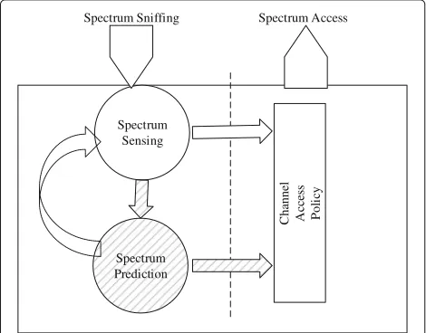
functions. These functions are represented by the sec-ondary user’s ability to perform spectrumsensing, deci-sion, sharing, and mobility [3, 4]. Spectrum occupancy prediction (SOP) models were proposed in DSA litera-ture to optimise cognitive cycle functions [5]. SOP models add agility, and adaptability to cognitive radio functions to optimise periodic spectrum sensing scheduling, and channel selection in spectrum decision (Fig.2) [3]. Simi-larly, SOP models allow the implementation of a proactive spectrum mobility strategy based on predicted occupancy patterns which avoids collisions with incumbent primary users [5,6].
SOP models for DSA systems broadly target occupancy parameters such aschannel availability, i.e. prediction of channel status as idle or busy, as well as,duty cycle, i.e. prediction of the average fraction of time the primary user is occupying the channel [7, 8]. Measurements on spectrum occupancy show as in Fig.3that spectrum pre-diction is much required to improve spectrum utilisation efficiency. The common motivation for SOP techniques is to minimise the accumulatedtime delaydue to cogni-tive cycle processing. By predicting the channel status in
Fig. 1An example of spectrum sensing and access in a typical DSA time-slotted system
advance, more processing time is available for spectrum sensing, decisions, and mobility [5]. SOP models address
prediction eitherexplicitly [9–11] or implicitly. Implicit approaches present SOP models as primary/secondary user activity models. In this review, we address both implicit and explicit formulations as statistical SOP models. Statistical SOP models proposed for spectrum occupancy analysis include Poisson processes [12, 13], Bayesian prediction [9,14], and linear regression [15,16]. Machine learning-based techniques have also been pro-posed for modellearningincluding neural networks, time regression, and space vector machines [5,17,18]. The sur-veys in [5,6] provide a good taxonomy of primary user’s
Spectrum Prediction Spectrum
Sensing
C
h
anne
l
A
cces
s
Po
li
cy
Spectrum Access Spectrum Sniffing
Fig. 2Prediction spectrum prediction in dynamic spectrum access framework
activity model collection. This review abstracts and con-solidate SOP models in DSA systems, and extends the aforementioned works.
Our contribution in this review paper is a consol-idated top-down classification of spectrum occupancy prediction. We present SOP taxonomy in a sequential prediction-based framework. This allows the authors to dissociate the spectrum prediction model from the appli-cation assumptions. In other words, this review paper addresses spectrum prediction model selection based on the theoretical sequential prediction stochastic class. The review places techniques adopted in literature into cate-gories based on their theoretical predictor classes. This classification approach highlights candidate prediction techniques suitable for SOP scenarios not extensively covered in current literature. Firstly, we review the fun-damentals of statistical prediction. Then, based on the stochastic mixture model framework, we review para-metric and non-parapara-metric approaches for underlying stochastic source assignment. Secondly, we describe spec-trum occupancy prediction in terms of the stochastic class assignment. We extend mixture model formula-tion to cooperative spectrum occupancy predicformula-tion using decision (hard) and data (soft) fusion techniques. Finally, we elaborate on additional theoretical and practical challenges of sequential spectrum occupancy prediction implementation.
In Section 2, we outline the fundamentals of statis-tical sequential prediction and detail relevant aspects in section Section 3. A brief review of empirical and statistical-based approaches for SOP modelling is pre-sented in Section 4. Then, we provide a review of cur-rent spectrum occupancy techniques in Sections 5, 6, and 7, respectively. This is followed by a review on cooperative spectrum prediction and fusion rules in Section8. Lastly, we list the challenges in spectrum occu-pancy prediction in Section 9, and concluding remarks in Section10.
2 Background
Fig. 3Power measurement campaign sample for Melbourne LTE system measurements [8]
definition of the sequential prediction problem is [19,20,23,27]:
Let a predictor receive a series of sequential observations xt−1 = {x1,x2...,xt−1}drawn from a sample spaceX. At
time instant t, the predictor performs an action atbased on the previous observations xt−1before the observation xtis available. Once xtis available, the predictor then updates the loss function l(at,xt).
The loss function l(at,xt) is a distance measure, e.g.
a squared error l(at,xt) = (xt − at)2. The action at
is generally assigned at = ˆxt (where xˆt is the
predic-tor’s guess ofxt) for “next event prediction”. Alternatively, at can represent the confidence in next event
predic-tion, i.e. the conditional probability at = pt
xt|xt−1
of one-step ahead prediction, given a series of obser-vations up to t −1. General loss function assignments transform sequential prediction problem into a decision problem [20,27].
There are two main formulations of the sequential pre-diction problem. The first isclassical predictionwhere the underlying source is assumed known, and the observa-tions are assumed identically distributed (not necessarily independent). The second formulation isuniversal
pre-diction, where no specific assumptions are made about
how the observed series is generated1. Conceptually, uni-versal prediction compares the designed predictor to an indexed set M of stochastic sources (e.g. distributions, codes, or polynomials). The true observation generating mechanism is generally assumed to be a member of the
predictorstochastic source setM[20,28]. The universal prediction algorithm is expected to perform at least as well as thebestmember of setMin terms of prediction loss [19,29,30]. The universal predictor is not necessar-ily a member ofM[30], but can be created as a mixture
of predictor setM[31]. Universal prediction formulation can be summarised as:
LetMbe an indexed set of arbitrary predictors. There exist prediction strategies for each sequence xt−1that can possibly be realised, which can predict essentially as well as the predictor inM that turns out to be best for that sequence “with hindsight”[19,30].
For example, a universal predictor may be compared to (or constructed from) a parametrised stochastic set
{Pθ,θ ∈M}such as a set of memoryless Poisson sources, a finite set ofkth-order Markov models, or a set of autore-gressive models of orderp[19,20,23,29]. However, the sequential predictor performance generally depends on the predictor setMclass “complexity” or richness, which quantifies the class type, size, and statistical regression between observations [19,20,23,29]. Thus, a set of finite kth-order Markov models is more practical for the predic-tor design than the set of all arbitrary order Markov mod-els due to the set size (see [20] for universality guarantee and indexed class size). If the predictor utilises Bayesian methods, a well-knownBayesian mixture model is con-structed as a weighted linear sum of the parametrised sources. Bayesian mixture models are the most common algorithms for predictor design (see Bayesian mixture models and redundancy-capacity theorem for optimal-ity analysis [20, 23, 28, 31]). However, they are by no means the only available methods, nor perform well for all arbitrary loss functions [19,29,30]2.
3 Statistical prediction
is categorised based on the assumptions about the exis-tence or non-exisexis-tence of an underlying stochastic source, see [19,20,23,29]. Statistical prediction is commonly pre-sented under either probabilistic or deterministic settings. Prediction loss function, regret, and redundancy are dis-cussed in Subsection3.3, while Subsection3.4provides an overview of Bayesian-based techniques.
3.1 Probabilistic settings
The classical definition of the sequential prediction problem assumes an arbitrary known stochastic process
{Pθ, θ ∈M}is responsible for generating the observations
xt[21,32,33]. Accordingly, optimal prediction is formu-lated as the minimisation of the expected value of the pre-dictor loss function [20,23,27,28,34]. For example, if{Xt}
is an arbitrary parametrised random source, the action
at = ˆxtis set as next observation prediction, and the loss
function is the squared distancel(at,xt) = E(at−xt)2
then the optimal predictor will always choose the con-ditional mean as it is predicted value. One of the most well-known techniques that utilises this approach is the Kalman filter [24,35,36] (see Section6). Practically, the underlying stochastic process are unknown, so a
replace-ment stochastic assignreplace-ment Q is created based on the
predictor setMof stochastic predictors. The performance of the designed sequential predictorQis compared to the best predictorPin the classM. The designed predictorQ has asymptotically small prediction regret compared toP [29,30].
3.2 Deterministic settings
There are two sequential prediction approaches when the underlying source is assumed deterministic. The first iscurve fitting, where a deterministic functionf(x)
is assumed responsible for generating the observations. Curve fitting generally exploits statistical regression in the observation series. Moving average and autoregres-sivelinear models (see Section7) are commonly used for deterministic settings prediction. The second approach seeks a universal deterministic predictor. The predictor avoids over-fitting the predictor to a specific sequence, i.e in deterministic settings, a predictor that is applica-ble to different sets of sequences [20,37]. The predictor class setMis a set of polynomials or code sequences. This construction avoids probabilistic assumptions about the observation source. However, when the designed predic-torQis constructed from the predictor set classM, a prior probability distribution is often assumed [19,30].
3.3 Loss function and regret
One step-ahead prediction commonly seeks the estimated state value at the next prediction slot a = ˆx. Alterna-tively, the action is setat = pt
xt|xt−1as a conditional probability assignment to measure the confidence in next
step prediction. Probabilistic prediction assignment pro-vides more information about the state of the system compared to next event prediction. The loss in predic-tion is measured between the designed predictor’s guess and the true value ofxt. Absolute, squared distance
mea-sures are common for next event prediction, while log distance is commonly used for probabilistic settings pre-diction. However, 0/1 loss function poses a challenge to several universal prediction algorithms including Bayesian mixture models [29,30].
The predictor regret expresses the instantaneous loss due to choice of probability assignment Q rather than the true source P. Subsequently, redundancy loss refers to the statistical expectation of regret for an observation sequence of lengthn[20,27]. For example, if a sourceQis used in place ofP, and a self information loss function is assumedat=pt
then the redundancy loss limit to be achieved by an opti-mal predictor is the entropy rate of the source H(P)
[20,27]. In other words, no additional loss due to the use ofQ [29, 30]. KL-divergence is commonly used to mea-sure performance distance and can be defined by thecross
entropybetweenPandQas
dt
dt is the instantaneous Kullback-Leibler (KL)
diver-gence, and Dn is the total distance counterpart [20,38].
Other possible choices for distance between P and Q are absolute, squared, Hellinger, and absolute divergence distances [28].
3.4 Bayesian methods for source assignment
Bayesianmixturemodels with self-information (entropy) loss were extensively studied in information and cod-ing theory [28,31,34]. Bayesian algorithms are minimax optimal and are universal under self information loss functions [20, 23, 27]. They perform well under both probabilistic and deterministic non-stochastic settings [20,27,28,38,39]. Probability source assignment forQis eitherparametricornon-parametric. The former assumes a single parametrised source Q=Pθˆin the predictor setM, while the later assumesQwas a mixture of sources with prior{w(θ),θ ∈M}[27]. Mixture source assignment utilises a weighted linear sum of distributions{Pθ,θ ∈M} with a prior distribution on the predictor index setM[20,23]. Using a non-negative normalised weighting function
w(θ). The mixture model density function is defined as
Qwxt=
Mw(θ)Pθ
The challenge in such models is the appropriate choice of the weights w(θ), i.e the prior distribution of the parameter θ ∈ M. Upper and lower loss bounds for Bayesian mixtures are defined using minimax and max-imin approaches [20,27]. Mixture models differ in terms of the size of the predictor index classC, stochastic class typePθ, and mixture priorw(θ). Different mixture models can be grouped into the four approaches:
3.4.1 Plug-in approach
This approach can be considered as a mixture model with the number of mixtures C = 1. The underlying source is assumed to be a single parametrised byθ. The chosen predictorPθˆprobability function is created by estimat-ing the value ofθˆbased on the seriesxt−1. The parameter
ˆ
θt = ˆθtxt−1can be estimated using a maximum
likeli-hood estimator [20,24]. However, plug-in approaches are heuristic and lack theoretical justification [20,23].
3.4.2 Finite mixture models
In finite mixture models, the replacement sourceQwis a sum of finite number of stochastic sources. The number of mixturesC<∞is generally decided beforehand based on the application objectives or through trial and error with different values ofC. Prior distribution often set in advance (uninformative uniform distribution is common choice).
Qwxt= C
i=1
Pθi(x t)w(θ
i), θi∈ {θ1, ..,θC}
Expectation-maximisation (EM) algorithm is used to estimate the parameter setθ ∈M[24,40,41].
3.4.3 Kernel density estimation
Kernel density estimation places akernel, i.e a function that satisfies probability density axioms on each obser-vation sample. The samples are assumed independent and identically distributed. The stochastic source Qw is defined as
Qwxn= 1 nh
n
t=1
K(x−xt)
h > 0 is the smoothing parameter, and the kernelK(., .) is a non-negative density function. Uniform, triangular, Epanechnikov, and normal kernels are some of common choices. [24,40,41].
3.4.4 Infinite mixture models
When the classMsize is infinite, the prior distribution on θis a smooth continuous function. The prior distribution is generally assumed drawn from a hyper-parametrised distribution, i.e. a probability distribution over proba-bility distributions. A common non-parametric Bayesian method is the Dirichlet processD(α,G), whereαis con-centration parameter, andGis the distribution overθ ∈
M. Samples ofθtat each time instanttare calculated
iter-atively fromGusing Monte-Carlo Markov chain methods. Infinite mixture model allows dynamic classification of data into clusters without having to specify the number of clusters in advance [40–42].
4 Review
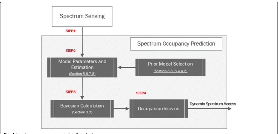
The flow chart in Fig.4highlights the temporal sequence spectrum occupancy prediction process presented in this section. This section focuses on model selection, while
the next three sections address selected model classes. We present current spectrum occupancy prediction tech-niques using the statistical sequential prediction def-inition. Current spectrum occupancy research can be broadly divided into measurement campaigns and statis-tical occupancy modelling. Notably, spectrum measure-ments are often used to estimate the selected SOP model parameters. For the spectrum prediction either the mea-surements or the models can be used.
4.1 Spectrum measurement campaigns
A spectrum measurement campaign is an empirical data collection conducted for specific scenarios, e.g. indoor/outdoor, to collect spectrum occupancy samples on pre-selected frequency bands, e.g television white bands/cellular phones. Statistical analysis and estima-tion are conducted to generate an approximate statisti-cal description of average power or channel occupancy. Though such modelling captures real-life spectrum occu-pancy scenarios, it is riddled with sampling inaccuracy, as well as spectral, spatial, and temporal dependency. How-ever, the data collected in these measurement campaigns are utilised to infer a suitable class setMfor the predic-tor design [7,8,43,44]. Campaigns in Hong Kong in [44] and Melbourne [8] assessed spectrum occupancy patterns for a large section of radio spectrum. The survey by Chen and Oh [7] provides an intensive review of several mea-surement campaigns for selected wireless communication technologies.
Figure 3 presents raw spectrogram results of spec-trum monitoring experiment conducted in three different urban environments in Melbourne metropolitan [8]. The spectrum campaign addressed spectral allocation for cog-nitive radio device-to-device communications and small cell networks. The spectrum occupancy is quantised by comparing the received signal level to an adaptive detec-tion threshold based on the noise power. Raw samples col-lected over all frequency sweeps are shown for three urban environment class. The work results indicated that fre-quency range 402–460 MHz and 520–820 MHz (vacated analogue TV band) are suitable candidate for DSA appli-cations [8].
4.2 Statistical occupancy modelling
Alternatively, statistical occupancy modelling estimates the observation generating mechanism often based on empirical samples. The scheme utilises a prior belief about the occupancy state and updates such belief as new observations are available. Given the estimated statistical model, spectrum occupancy prediction at future instances is achievable. Such models examine several statistical techniques with a major literature focus on Markov pro-cesses [10,45], Poisson processes [12,13], Bayesian mod-els [9,14], neural networks [5, 11, 46], linear regression
[15, 16], space vector machine [47], pattern mining [48,49], and dictionary-based prediction [9]. In a sequen-tial prediction framework, these techniques represent different parametrised predictor classes.
4.2.1 Prediction model selection
Parameters studied by spectrum occupancy modelling are (i) channel status, i.e prediction of the spectrum status as idle or busy, (ii) duty cycle, i.e. prediction of average fraction of time the spectrum channel is occupied, or (iii) signal/power, i.e. prediction of the power level on a spe-cific channel. These occupancy series are modelled based on assumptions about their state space, loss function, and predictor action. For instance, channel status observation series can be modelled as an ON/OFF (2-state model) binary source model X = [0, 1], or more (e.g. 3-state model). Similarly, the predictor action at is commonly
modelled as one-step ahead state prediction, i.e.at= ˆxtor
as a probabilistic assignment, i.e.at = p
xt|xt−1. Com-mon choices for loss functions are self information, 0/1 loss and mean square error, while regret and redundancy often adopt KL-divergence. However, the loss function in each proposal is often formulated based on the intended application (e.g. throughput, sensing accuracy, or hand-off success rate). Performance comparison metrics such as secondary user’s throughput, spectrum interference and wastage, and probability of error (or mean square error) are generally defined based on the probability density of the one step-ahead prediction, as well as, the predic-tion loss funcpredic-tion. For example, the probability of incor-rect prediction of an available spectrum hole generally describe spectrum interference or spectrum wastage [50]. Consequently, spectrum occupancy prediction mod-elling is essentially the selection of a classMof predictors or the mixture of sources from classM. The choice of the predictor class is limited by the application requirements and constraints. For example, a set of finite kth-order Markov models is more practical for the predictor design than the set of all arbitrary order Markov models, due to the set size. Moreover, HMM model is suitable for finite state occupancy models one step-ahead prediction given the errors in the wireless channel, while Kalman fil-ter is a more suitable for infinite state space scenarios. Kernel density estimation is rarely proposed for on-line prediction, but can be used to construct the probability density of selected predictor class. Ultimately, the sequen-tial predictor performance depends on the predictor set
M “complexity” or richness, which quantifies the class type, size, and statistical regression between observations [19,20,23,29].
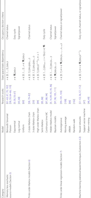
ON/OFF) or infinite set (e.g. real spaceR) are presented. Additionally, state regression and dependency on previ-ous events (e.g. first order Markov chain) are presented. Finally, occupancy series are displayed in the last column.
4.2.2 Prediction models classification
By dissociating the implementation requirements and assumptions from the stochastic components of the spec-trum prediction model, the authors distinguish three major categories of parametrised predictor classes used in literature:
1. Memoryless stochastic sources classes (single source). This category contains a diverse set of parametrised sources including Bernoulli, Binomial, Poisson, exponential, uniform, and normal
distributions. Such models are better suited for traffic
such asinternet of things, telemetry, and applications
that use radio spectrum.
2. Finite order Markov chain class (finite source memory). The dominant choice is first order Markov chain with finite/infinite state space such as hidden Markov model, Kalman filters, and particle filters. These models are better suited for applications such as TCP/IP traffic.
3. Finite order linear regression source class. Autoregressive (AR) and moving-average (MA) models along with ARMA, and ARIMA models assume linear regression in the observation series. This set of models is also suitable for TCP/IP traffic, with the advantage of low complexity
implementation.
4. Machine learning-based techniques including neural networks, support vector machines, and pattern mining can be used for massive access network scenarios.
Table 2 highlights few major advantages and disad-vantages of different spectrum occupancy prediction categories. For example, stochastic memoryless modes ignores temporal correlation of the data, but suitable for low complexity single PU sparse channel usage sce-narios. Similarly, finite Markov models are suitable for heavy-tail channel usage scenarios such as multimedia transfer. Markov-Bayesian mixtures can be used to model scenarios with multiple primary and secondary users. Finally, linear regression models exploit further past mea-surements with less complexity compared to finite state Markov models.
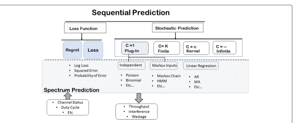
Figure5 summarizes the sequential prediction theory presented in Section 3 and maps current SOP tech-niques. The number of mixture sourcesCin the replace-ment source assignreplace-mentQdifferentiates mixture models (Subsection 3.4). The figure conceptually illustrates the
modelled occupancy series as an input, where the selected mixture model produces the desired performance measure based on the selected loss function. Model classification presented in this section is displayed under mixture model framework. We present a review of cur-rent spectrum prediction techniques for each category in the next three sections. Section5presents single memory-less source approaches, Section6handles Markov-based models, while Section7presents linear statistical regres-sion based prediction.
4.3 Machine learning-based techniques
Machine learning, data mining, and pattern recogni-tion algorithms are based on existing statistical inference models. Kobayashi et al. [[24], Chapter 21] discusses the statistical aspects of machine learning. Several classifica-tion and predicclassifica-tion techniques are a numerical methods based on a statistical prediction model. For example,
arti-ficial neural networksandHMMare numerical solutions
of Bayesian /Markov models (particularly particle filer solutions). Similarly, support vector machine are numeri-cal solutions of linear regression models.
Artificial intelligence and machine learning in spectrum prediction generally address the learning of predictor class parameters. The methods improve likelihood esti-mation for spectrum prediction problems with large sample size. For example, neural network genetic algo-rithms can be used for maximum likelihood estima-tion of HMM parameters [51]. Neural networks-based techniques are presented extensively in cognitive radio networks [18,51–55], with application on spectrum pre-diction presented in [56, 57]. Support vector machines [47], pattern mining [48,49], and dictionary-based predic-tion [9] were suggested for spectrum prediction and user activity modelling. The surveys in [17,18,54] discuss arti-ficial intelligence and machine learning applications for dynamic spectrum access.
5 Spectrum occupancy prediction with memoryless stochastic source models
In this category, the observations are assumed indepen-dent and iindepen-dentically distributed (i.i.d) random variables drawn from a single parametrised stochastic source. The series xt−1 has no conditional dependency on the pre-diction of xˆt, i.e. models fall under this category are memoryless. Practically, one-step ahead prediction is not possible with such models. Thus, it is often combined with time correlated assumptions (e.g. Poisson Markov chain [58,59]) or used to estimate the stochastic source prob-ability density function Qw from a training sequence. Models adopted in SOP proposals include the following:
Table 2Comparison of spectrum prediction categories
Category Advantages Disadvantages
Memoryless stochastic Low complexity Limited to sparse spectrum usage
source models (Section5) Closed form solution for sparse Limited to single primary spectrum usage scenarios user scenarios
Easier/convenient model to adopt May not describe real world channel occupancy status Finite order Markov models (Section6) Expandable to various PU/SU scenarios Require sufficient measurements
for model training Applicable to heavy-tailed channel traffic Complexity depends on the
order of the model Higher accuracy with manageable
number of parameters
Finite order linear regression models (Section7) Expandable to various PU/SU scenarios Expandability increases the number of model parameters Approximation of probabilistic Require sufficient measurements for model training model to linear equation model
only the values 0 or 1 representing failure and success, respectively. The series x1,x2. . .xt−1 is assumed to be
independent and identically distributed Bernoulli random variables, with probability mass function parametrised by
ρ[24,60]:
f(k;ρ)=ρk(1−ρ)(1−k), k∈ {0, 1}
Wherekis the number of trials, andρis the probability a certain outcome, e.g.ρ=p(Xt=1).
Binomial distribution models the probability of exactly
ksuccess inntrials, yielding the probability mass function parametrised byρas
f(k;ρ)=Cknρk(1−ρ)(n−k), Ckn= n! k!(n−k)!
Poisson distribution describes the probability of a num-ber ofkevents in a time period with a constant average rateλ= nk [24,60]:
f(k;λ)= λ
ke−λ
k! , k∈ {0, 1,. . .}
Exponential distribution. The interval between events in a Poisson distributed process follows the negative expo-nential distribution parametrised by λ, with probability density function [24,60]:
f(x;λ)=λe−λx, x≥0, λ >0.
In spectrum occupancy literature, memoryless sources are not often used for one-step ahead prediction. How-ever, this class of stochastic sources is frequently used to describe primary user activity. Bernoulli process have
been proposed in [61–63] to describe ON/OFF spectrum occupancy in spectrum sensing/access proposals. Sim-ilarly, Poisson process have been proposed in [58, 64] (2 states) and [59] (3 states) to model the arrival/departure process of the primary user. Exponentially distributed duty cycle models were presented based on queuing the-ory in [58,59]. Similarly, proposals in [65,66] suggested a non-exponential service time as a result for multiple pri-mary users scheduling. In [9], an exponential distribution to model inter-arrival time of the primary users was pro-posed to design a secondary contention algorithm. Joint cognitive radio spectrum sensing and prediction model in [67] proposed an exponential primary user prediction and estimated spectrum opportunity wastage and inter-ference. Other primary user modelling efforts utilised an identical approaches with i.i.d events, but employed different probability distributions such as log-normal dis-tribution [43,68], uniform distribution [69], and binomial distribution [67, 70]. The choices were generally moti-vated by physical layer assumptions.
6 Spectrum occupancy prediction with finite order Markov models
Various Bayesian-based techniques utilise different assumptions about the observation sample space, the statistical regression, and the underlying stochastic pro-cess. The case when the probability of current event xt
only depends on the probability of previous event xt−1,
i.e. pxt|xt−1 = p(xt|xt−1) is called Markov property
[24]. Markov-based construction is attractive due to the desirable convergence properties of Markov chain-based models [71–74]. Markov chain and partially
observ-able Markov models are commonly used for spectrum
occupancy modelling. Markov processes also include
semi-Markovprocesses suchM-order Markov chainwith
dependence on m previous events, i.e. xt−m, or explicit
duration Markov chain (a form of continuous-time
Markov chain), where the time spent on each state is not exponentially distributed [24, 75]. The main difference between proposals is the number of states assumed by different models and the proposal’s loss function.
Bayesian Markov model General Markov-based model
in estimation theory utilises a Bayesian model framework as [76]:
The first equation is Chapman-Kolomogrov prediction equation, the second is Bayes rule update, while the last equation is normalisation factor [76]. This model is labelled doubly stochasticas it accounts for measure-ment error in xt−1 by defining the observation series
yt−1, while xt−1 is defined as the latent variable series.
The latent state model is defined by the non-linear
function [xt=ft(xt−1,vt)], and vt an independent
addi-tive noise source. xt is distributed based on the
prob-ability p(xt|xt−1) defined as latent state Markov prior.
The observations are defined as the dependent variable
yt=ht(xt,ut) , where ht is a non-linear function, and utis an independent additive noise source (measurement
error) [24]. The observation variable is distributed accord-ing top(yt|xt), defined as the observation likelihood
prob-ability. The conditional posterior probability pxt|yt−1
is recursively calculated from the prior and likelihood probabilities from an initial state distributionp(x0). The
equation set simplifies the probability assignment in the formpxt|yt−1=pxt|xt−1,yt−1
pxt−1|yt−1
(Markov property). When implementing such model, the density
pxt|yt−1is either estimated using the prior/likelihood function or using kernel density estimation [36,76].
Markov chain process is the simplest Bayesian Markov model. It is assumed to be fully observable, and finite. Markov chain process is parametrised bytransition prob-abilityand initial state distribution. Each element in the transition matrix is the probabilitypijt, i.e. the probability of being in statejat timetgiven the system is currently in stateiat timet−1 [24,76–78].
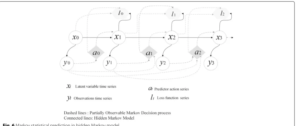
Hidden Markov model (HMM) is partially observable
Markov chains, i.e. observing a Markov chain through a noisy channel [24, 75]. HMM employs two finite sam-ple sets for latent variables X and observations Y. The additional conditional probability of a system is at statei
(xt=i) to emit an observation (yt=j) is referred to aseij
or theemissionprobability. Figure6displays a snapshot of HMM state transition (connected lines).
Kalman filter is the optimal solution for linear Gaussian state space Markov-based models [24,36,76]. Non-linear predictors are often a sub-optimal variation of Kalman fil-ter, such as extended Kalman filfil-ter, and unscented Kalman filter [24,35,36].
Bayesian particle filters Particle filter methods utilise Monte-Carlo Markov chain (MCMC) to approximate the conditional posterior probability assignment pxt|yt−1
or the full posterior probability pxt|yt−1. They utilise
Fig. 6Markov statistical prediction in hidden Markov model
In the spectrum modelling literature, Poisson Markov chain-based proposals in [58, 59] studied primary user interference and wastage. Two-state [79–83] and three-state discrete-time Markov [59] chain have been pro-posed to model the primary-secondary users stochastic behaviour. Similarly, higher-order Markov chains in [84] were used to detect the primary user traffic pat-tern. Explicit duration semi-Markov chains with gener-alised distribution of duty cycle time modelled primary user’s inter-arrival time in [85, 86], while continuous time Markov chain modelled primary user behaviour in [87, 88]. Moreover, hidden Markov model received wide attention in spectrum occupancy prediction literature [9, 14, 83, 89–93]. Liu et al. addressed the prediction confidence, and the error of a continuous time Markov chain model with Erlang-2 distribution model for primary user’s activity [94]. K-step ahead prediction was studied in [95,96] assuming a non-stationary HMM. Finally, works in [97, 98] utilised regularised particle filters with Ker-nel density estimation to model primary user activity in multi-primary and secondary user cases.
7 Spectrum occupancy prediction with finite order linear regression models
A special case of the general non-linear statistical regres-sion forpxt|xt−1, linear regression models focus on the
linear dependency between the random variablesxt, and xt−1[24]. Autoregressive modelAR(p= 0), and moving average (MA) (q = 0) are special cases of autoregres-sive moving-average. ARMA modelARMA(p,q) can be written as [24,60]
xt=c+ηt+ p
i=1
φixt−i+
q
i=1
θiηt−i
Wherecis a constant that can be replaced withμ =
Ex{xt}. ηt is a noise random variable that represents
the uncertainty in sampling. φi,θi are the
autoregres-sive, and moving average parameters.p,q are the order of the autoregressive and moving average components. Autoregressive integrated moving-average (ARIMA) pro-cess generalises the ARMA model toARIMA(p,d,q)and written as [24,60]
1−
p
i=1
φiLi
(1−L)dxt=
1+
q
i=1
θiLi
ηt
WhereLi(xt) = xt−i is the time lag operator, xt = xt−xt−1=(1−L)xtis the difference operator, anddxt= (1−L)dxt is the generalised difference operator. Setting
the differencing degreed=0 in ARIMA model will result in ARMA model, while settingp=q=0, d=1 results in a random walk model. ARMA and ARMIA assume no specific underlying stochastic process, but provides the regression between observation samples.
An autoregressive with Gaussian distributed random variables was used to model spectrum occupancy in [99–101]. Similarly, moving-average [100] and ARIMA [66] were proposed for spectrum occupancy status mod-elling. Random walk model was proposed in [102] to model spectrum occupancy duty cycle. Finally, an autore-gressive model of decimal equivalent of a binary series model was proposed for primary user activity in [103].
8 Cooperative spectrum prediction
Spectrum prediction in single secondary user environ-ment is local spectrum prediction. Consequently,
coop-erative spectrum prediction in multi-user environment
cooperative prediction refers to the case when secondary users have identical detection performance in terms of channel conditions, e.g. signal to noise ratio. While hetero-geneouscooperative prediction refers to the general case of non-identical secondary user detection performance. The latter scenario incorporates additional dependency on the spatial distribution [93]. Cooperative prediction fusion proposals are commonly classified into hard and soft fusion techniques.
8.1 Hard prediction fusion
ForRcooperative users with a binary observation series
dr ∈ {0, 1}, the predicted occupancy state at each
coop-Where 1[..] is the indicator function. The three main rules for thresholdMare:M= 1 the logical OR,M=N
the logical AND, andM = N/2 is the majority decision rule.
8.2 Soft prediction fusion
If the data shared by each cooperative user r at time instance t is defined asdr = ar(t) = pr
xt|yt−1, or
dr = ˆxk(r). Then, the total cooperative decisionDR(t)at
each time instanttcan be defined as a finite weighted sum of each user’s data. The soft fusion predictionDRcan be
defined as
Wherewr is a prior distribution on theRcooperative
user. Soft fusion-based formulation on the predictive pos-terior probabilitypr(xt|yr,1:t−1)can be modelled as a linear
mixture model. Let a non-negative normalised weighting function bew(θ)parametrised byθ, the mixture model is defined as
For a finite number of userRthe mixture sum is
pw
A diverse collection of techniques can be adopted for the priorwθ selection. Equal gain, maximal ratio, and selec-tion combining fusion are the most common of these soft fusion techniques.
8.2.1 Equal gain fusion
Equal gain combining assumes all secondary users have an equal “weight”, i.e.wr = 1R,r∈ {1, 2, ..,R}, i.e.θ =R. This
fusion strategy ignores the heterogeneous nature of sec-ondary user’s detection/prediction performance, as well as their spatial distribution.
Selection combining uses the decision of the user with the best channel condition, e.g. signal to noise ratio ρ. The method overrules decisions made by all other cooperative user and uses the best user decisions [30].
pw
Maximal ratio combining utilise SU signal to noise ratio ρrin the priorw(θ), i.e.θ =ρr:
wr(ρr)= Rρr r=1ρr
Cooperative fusion of channel access decisions has been studied extensively in spectrum sensing using hard and soft fusion techniques [104]. But a limited number of stud-ies focused on applications for one step ahead prediction. In our previous work on cooperative prediction [93], we extended prediction error performance analysis for HMM predictors [83]. In [98], cooperative prediction was pro-posed as a coalition game. Similarly, the studies in [67] proposed a majority hard fusion based cooperative predic-tion for binomially distributed predicpredic-tions. Finally, Saad et al. [105] proposed a beta distribution prior for a linear Gaussian kernel density estimated PU activity. The study presented a trade-off between communication cost and prediction accuracy.
9 Spectrum occupancy prediction challenges The survey in [6] discussed the issue of occupancy mod-elling validity based on the type and amount of traffic pattern. The survey presented several scenarios of pos-sible implementation issues for primary user modelling. This section extends the survey, and presents theoretical challenges for SOP models.
9.1 Validity and complexity
have temporal, spectral, and spatial dependency. Pro-posed spectrum occupancy prediction models simplify assumption about spectral and spatial assumptions to avoid model complexity. To our knowledge, there are no multi-dimensional proposals for spectrum occupancy prediction. Moreover, the validity of any chosen model is generally questionable from dimensionality and universal-ity perspective, as any assumption about the underlying observation process may not fit the actual behaviour. Few spectrum measurement campaigns invalidated sev-eral short-term prediction assumptions. Thus, validation through empirical spectrum campaigns is essential for any spectrum predictor design [8, 10]. For example in [106], the popular i.i.d exponential duty cycle assump-tion is criticised as a model for short-term predicassump-tion. A Pareto distribution was proposed for long-term predic-tion, but short-term prediction was deemed application dependent, and technology specific.
Moreover, common challenges in sequential prediction theory are model over-fitting, and redundancy loss con-vergence guarantee. Model over-fitting refers to the case when a model is too complex, that renders it sensitive to small changes in observation statistics [19,20,23,29]. Model complexity constraints the applicability of the diction mode. The complexity of a specific class of pre-dictors, i.e. class size and statistical regression affects the predictor convergence guarantee to the desired redun-dancy loss bound (see redunredun-dancy-capacity theorem [20, 23, 28, 31]). Plug-in approaches simplify predictor design complexity using assumptions about the observa-tion generating mechanism to achieve optimal predictor design. For example, a set of finite kth-order Markov models are more practical for predictor design compared to the set of all arbitrary order Markov models. More-over, mixture models are more complex but allow empir-ical measurements-based source estimation. An example would be Dirichlet mixture process which often used to generate mixture prior distributions, but tracing con-vergence bounds becomes increasingly difficult for non-Gaussian mixtures for example [20,28,40]. Convergence bounds are calculated only for limited Bayesian mix-ture class/prior distribution pairs (for example, uniform prior/Epanchinkov kernel) [107].
9.2 Cooperation and contention
Cooperative spectrum prediction faces the practical issue of common control channel design [97]. The amount of data shared between users sets a trade-off between spectrum prediction accuracy and control channel capac-ity [97]. Common control design for cooperative spec-trum prediction in a multi-primary, user’s environment is yet to develop in the spectrum prediction litera-ture. Analysis of cooperative prediction using hierarchical Dirichlet processes is an interesting proposal to model
cooperative spectrum prediction, that is not explored in SOP literature [40].
Contention policy proposals for DSA systems are still under development in current literature. In single user case, reinforcement learning is suggested in some litera-ture sources to model the spectrum occupancy [50,108]. However, the study in [108] questions reinforcement learning as useful tool to improve spectrum occupancy modelling of their own spectrum campaign measure-ments. Multi-user game theory-based approaches are interesting candidates for multi-user spectrum prediction.
10 Conclusions
In this paper, we presented a comprehensive survey and classification of spectrum occupancy prediction (SOP) based on theoretical sequential prediction framework. To the best of authors’ knowledge, this review on spectrum occupancy prediction in literature is the first to con-solidate current techniques based on sequential predic-tion theoretical framework. This classificapredic-tion approach highlights candidate techniques suitable for SOP scenar-ios not extensively covered in current literature. In the paper, we presented the definition and fundamentals of statistical sequential prediction. Then, we addressed pre-dictor loss, regret, and Bayesian methods for underlying stochastic source assignment. Based on parametric and non-parametric mixture model framework, this paper classifies spectrum occupancy modelling approaches in literature based on predictor class selection. Predictor class selection categories of memoryless sources, Markov models, and linear regression models along with machine-based techniques were detailed machine-based on current SOP literature proposals. SOP cooperative prediction based on hard and soft fusion techniques was discussed for multi-user scenarios. Finally, spectrum predication theoretical and practical challenges were presented and highlighted candidate techniques.
Endnotes
1Probabilistic assumptions are made about the M
sources prior, and under probabilistic actionat
assump-tions see [19,29,30].
2The major cases are 0/1 loss function for
probabilis-tic action at and 0/1 loss for ON/OFF non-stochastic
observations, see [19,29,30] for analysis and [29,30,109] for Starkov codes, Hedge algorithm, and game theory approaches for sequential prediction.
Abbreviations
Acknowledgements
This research was supported under Australian Research Council’s Discovery Projects funding scheme (Cognitive Radars for Auto-mobiles, DP150104473). We would like to thank Dr. Akram Al-Hourani for Melbourne spectrum measurement campaign data.
Funding
Not applicable.
Authors’ contributions
HE contributed towards Section1to10. A/Prof. SK contributed to Section2. Prof. RJE contributed to Sections3and6. Prof. YCL contributed to Sections4, 8, and9. Dr. BR contributed to Sections2and3. All authors read and approved the final manuscript.
Authors’ information
The work of Y.-C. Liang is funded by National Natural Science Foundation of China under Grants 61571100, 61631005 and 61628103.
Ethics approval and consent to participate
Not applicable.
Consent for publication
Not applicable.
Competing interests
The authors declare that they have no competing interests.
Publisher’s Note
Springer Nature remains neutral with regard to jurisdictional claims in published maps and institutional affiliations.
Author details
1School of Engineering, RMIT University, 124 La Trobe St, 3000 Melbourne,
Australia.2Department of Electrical and Electronic Engineering, University of
Melbourne, Parkville, Melbourne, 3010 Australia.3University of Electronic
Science and Technology of China (UESTC), Chengdu 611731, China.
Received: 8 February 2017 Accepted: 25 December 2017
References
1. IF Akyildiz, W-Y Lee, MC Vuran, S Mohanty, NeXt generation/dynamic spectrum access/cognitive radio wireless networks: A survey. Comput. Netw.50(13), 2127–2159 (2006).http://dx.doi.org/10.1016/j.comnet. 2006.05.001
2. C Baylis, M Fellows, L Cohen, RJM II, Solving the spectrum crisis: intelligent, reconfigurable microwave transmitter amplifiers for cognitive radar. IEEE Microw. Mag.15(5), 94–107 (2014).https://doi.org/ 10.1109/mmm.2014.2321253
3. YC Liang, KC Chen, GY Li, P Mahonen, Cognitive radio networking and communications: an overview. IEEE Trans. Veh. Technol.60(7), 3386–3407 (2011).https://doi.org/10.1109/TVT.2011.2158673 4. IF Akyildiz, W-Y Lee, MC Vuran, S Mohanty, A survey on spectrum
management in cognitive radio networks. IEEE Commun. Mag.46(4), 40–48 (2008).https://doi.org/10.1109/mcom.2008.4481339 5. X Xing, T Jing, W Cheng, Y Huo, X Cheng, Spectrum prediction in
cognitive radio networks. IEEE Wirel. Commun.20(2), 90–96 (2013). https://doi.org/10.1109/mwc.2013.6507399
6. Y Saleem, MH Rehmani, Primary radio user activity models for cognitive radio networks: a survey. J. Netw. Comput. Appl.43, 1–16 (2014).https:// doi.org/10.1016/j.jnca.2014.04.001
7. Y Chen, H-S Oh, A survey of measurement-based spectrum occupancy modeling for cognitive radios. IEEE Commun. Surv. Tutorials.18(1), 848–859 (2016).https://doi.org/10.1109/comst.2014.2364316 8. A Al-Hourani, V Trajkovic, S Chandrasekharan, S Kandeepan, Spectrum
occupancy measurements for different urban environments. 2015 Eur. Conf. Netw. Commun. (EuCNC) (2015).https://doi.org/10.1109/eucnc. 2015.7194048
9. SJ Kim, GB Giannakis, in2013 5th IEEE International Workshop on Computational Advances in Multi-Sensor Adaptive Processing (CAMSAP). Dynamic learning for cognitive radio sensing (IEEE, Piscataway, 2013), pp. 388–391.https://doi.org/10.1109/CAMSAP.2013.6714089
10. Z Chen, N Guo, Z Hu, RC Qiu, Experimental validation of channel state prediction considering delays in practical cognitive radio. IEEE Trans. Veh. Technol.60(4), 1314–1325 (2011).https://doi.org/10.1109/TVT. 2011.2116051
11. L Yin, S Yin, W Hong, S Li, inMilitary Communications Conference (MILCOM). Spectrum behaviour learning in cognitive radio based on artificial neural network (IEEE, Piscataway, 2011), pp. 25–30.https://doi. org/10.1109/MILCOM.2011.6127671
12. J Lee, HK Park, Channel prediction-based channel aladdress scheme for multichannel cognitive radio networks. J. Commun. Netw.16(2), 209–216 (2014).https://doi.org/10.1109/jcn.2014.000032
13. W Pu, IF Akyildiz, Asymptotic queuing analysis for dynamic spectrum access networks in the presence of heavy tails. IEEE J. Sel. Areas Commun.
31(3), 514–522 (2013).https://doi.org/10.1109/JSAC.2013.130316 14. X Li, SA Zekavat, Cognitive radio based spectrum sharing: evaluating
channel availability via traffic pattern prediction. J. Commun. Netw.
11(2), 104–114 (2009).https://doi.org/10.1109/JCN.2009.6391385 15. VK Tumuluru, P Wang, D Niyato, Channel status prediction for cognitive
radio networks. Wirel. Commun. Mob. Comput.12(10), 862–874 (2012). https://doi.org/10.1002/wcm.1017
16. S Chen, L Tong, Maximum throughput region of multiuser cognitive access of continuous time Markovian channels. IEEE J. Sel. Areas Commun.29(10), 1959–1969 (2011).https://doi.org/10.1109/JSAC.2011. 111206
17. M Bkassiny, Y Li, SK Jayaweera, A survey on machine-learning techniques in cognitive radios. IEEE Commun. Surv. Tutorials.15(3), 1136–1159 (2013).https://doi.org/10.1109/surv.2012.100412.00017
18. A He, KK Bae, TR Newman, J Gaeddert, K Kim, R Menon, L Morales-Tirado, JJ Neel, Y Zhao, JH Reed, WH Tranter, A survey of artificial intelligence for cognitive radios. IEEE Trans. Veh. Technol.59(4), 1578–1592 (2010). https://doi.org/10.1109/tvt.2010.2043968
19. N Cesa-Bianchi, G Lugosi,Prediction, Learning, and Games. (Cambridge University Press, New York, 2006).https://doi.org/10.1017/
cbo9780511546921
20. N Merhav, M Feder, Universal prediction. IEEE Trans. Inf. Theory.44(6), 2124–2147 (1998).https://doi.org/10.1109/18.720534
21. H Bolfarine, S Zacks,Prediction theory for finite populations, Springer Series in Statistics. (Springer, New York, 1992). https://doi.org/10.1007/978-1-4612-2904-9
22. CE Shannon, Prediction and entropy of printed english. Bell Syst. Tech. J.30(1), 50–64 (1951).https://doi.org/10.1002/j.1538-7305.1951. tb01366.x
23. J Rissanen, Universal coding, information, prediction, and estimation. IEEE Trans. Inf. Theory.30(4), 629–636 (1984).https://doi.org/10.1109/tit. 1984.1056936
24. H Kobayashi, BL Mark, W Turin,Probability, random processes, and statistical analysis: applications to communications, signal processing, queueing theory and mathematical finance. (Cambridge University Press, New York, 2011)
25. J Ziv, A Lempel, A universal algorithm for sequential data compression. IEEE Trans. Inf. Theory.23(3), 337–343 (1977).https://doi.org/10.1109/tit. 1977.1055714
26. JL KELLY, A new interpretation of information rate. IRE Trans. Inf. Theory.
2(3), 25–34 (2011)
27. Kotł, W,owski, Grü,nwald, inIEEE Information Theory Workshop (ITW), 2012. Sequential normalized maximum likelihood in log-loss prediction (IEEE, Piscataway, 2012), pp. 547–551.https://doi.org/10.1109/ITW.2012. 6404734
28. M Hutter, Convergence and loss bounds for bayesian sequence prediction. IEEE Trans. Inf. Theory.49(8), 2061–2067 (2003).https://doi. org/10.1109/tit.2003.814488
29. G Shafer, V Vovk,Probability and finance: it’s only a game! Wiley Series in Probability and Statistics. (Wiley, New York, 2005).https://doi.org/10. 1002/0471249696
30. PD Grnwald, IJ Myung, MA Pitt,Advances in minimum description length: theory and applications (Neural Information Processing). (The MIT Press, Cambridge, 2005)
32. NN Cencov,Statistical decision rules and optimal inference (translations of mathematical monographs), vol. 53. (American Mathematical Society, Providence, 2000)
33. PP Vaidyanathan, The theory of linear prediction. Synth. Lect. Signal Process.2(1), 1–184 (2007).https://doi.org/10.2200/s00086ed1v01y 200712spr003
34. PH Algoet, The strong law of large numbers for sequential decisions under uncertainty. IEEE Trans. Inf. Theory.40(3), 609–633 (1994).https:// doi.org/10.1109/18.335876
35. EA Wan, RVD Merwe, inProceedings of the IEEE 2000 Adaptive Systems for Signal Processing, Communications, and Control Symposium. The unscented kalman filter for nonlinear estimation (IEEE, Piscataway, 2000), pp. 153–158.https://doi.org/10.1109/asspcc.2000.882463
36. B Ristic, S Arulampalam, NJ Gordon,Beyond the Kalman filter: particle filters for tracking applications. (Artech house, London, 2004) 37. JGD Gooijer, RJ Hyndman, 25 years of time series forecasting. Int. J.
Forecast.22(3), 443–473 (2006).https://doi.org/10.1016/j.ijforecast.2006. 01.001
38. TM Cover, JA Thomas,Elements of information theory. (Wiley, New York, 2006)
39. A Goldsmith, P Varaiya, Capacity, mutual information, and coding for finite-state Markov channels. IEEE Trans. Inf. Theory.42(3), 868–886 (1996).https://doi.org/10.1109/isit.1994.394696
40. RM Neal, Markov chain sampling methods for Dirichlet process mixture models. J. Comput. Graph. Stat.9(2), 249–265 (2000).https://doi.org/10. 1080/10618600.2000.10474879
41. M Dudí, SJ Phillips, RE Schapire, inLearning Theory. Performance guarantees for regularized maximum entropy density estimation (Springer, Berlin, Heidelberg, 2004), pp. 472–486
42. YW Teh,Dirichlet Process. (C Sammut, GI Webb, eds.) (Springer, Boston, 2010), pp. 280–287.https://doi.org/10.1007/978-0-387-30164-8 43. M Wellens, P Mähönen, Lessons learned from an extensive spectrum
occupancy measurement campaign and a stochastic duty cycle model. Mob. Netw. Appl.15(3), 461–474 (2010).https://doi.org/10.1007/ s11036-009-0199-9
44. MH Islam, CL Koh, SW Oh, X Qing, YY Lai, C Wang, Y-C Liang, BE Toh, F Chin, GL Tan, W Toh, in2008 3rdInternational Conference on Cognitive Radio Oriented Wireless Networks and Communications (CrownCom 2008). Spectrum survey in singapore: occupancy measurements and analyses (IEEE, Piscataway, 2008), pp. 1–7.https://doi.org/10.1109/crowncom. 2008.4562457
45. W Tang, J Zhou, H Yu, S Li, A fair scheduling scheme based on collision statistics for cognitive radio networks. Concurr. Comput. Pract. Experience.25(9), 1091–1100 (2012).https://doi.org/10.1002/cpe.2879 46. C Xianfu, Z Honggang, AB Mackenzie, M Matinmikko, Predicting
spectrum occupancies using a non-stationary hidden Markov model. IEEE Wirel. Commun. Lett.3(4), 333–336 (2014).https://doi.org/10.1109/ LWC.2014.2315040
47. C Xu, H Jianwei, Evolutionarily stable spectrum access. IEEE Trans. Mob. Comput.12(7), 1281–1293 (2013).https://doi.org/10.1109/TMC.2012.94 48. P De, Y-C Liang, Blind spectrum sensing algorithms for cognitive radio
networks. IEEE Trans. Veh. Technol.57(5), 2834–2842 (2008).https://doi. org/10.1109/tvt.2008.915520
49. P Huang, C-J Liu, L Xiao, J Chen, Wireless spectrum occupancy prediction based on partial periodic pattern mining. 2012 IEEE 20th Int. Symp. Model. Anal. Simul. Comput. Telecommun. Syst.25(7), 1925–1934 (2012).https://doi.org/10.1109/mascots.2012.16
50. S Arunthavanathan, S Kandeepan, RJ Evans, in2013 IEEE Globecom Workshops (GC). Reinforcement learning based secondary user transmissions in cognitive radio networks (IEEE, Piscataway, 2013), pp. 374–379.https://doi.org/10.1109/glocomw.2013.6825016 51. J Yang, H Zhao, X Chen, inIEEE 2nd International Conference on Computer
and Communications (ICCC). Genetic algorithm optimized training for neural network spectrum prediction (IEEE, Piscataway, 2016), pp. 2949–2954.https://doi.org/10.1109/compcomm.2016.7925237 52. S Ni, X Bai, Z Wang, B Guo, inIEEE International Congress on Image and
Signal Processing, BioMedical Engineering and Informatics (CISP-BMEI). A new method of cognitive radio spectrum prediction research (IEEE, Piscataway, 2016), pp. 982–986.https://doi.org/10.1109/cisp-bmei.2016. 7852855
53. A Agarwal, S Dubey, MA Khan, R Gangopadhyay, S Debnath, in2016 International Conference on Signal Processing and Communications (SPCOM). Learning based primary user activity prediction in cognitive radio networks for efficient dynamic spectrum access (IEEE, Piscataway, 2016), pp. 1–5.https://doi.org/10.1109/SPCOM.2016.7746632 54. C Clancy, J Hecker, E Stuntebeck, T O’Shea, Applications of machine
learning to cognitive radio networks. IEEE Wirel. Commun.14(4), 47–52 (2007).https://doi.org/10.1109/MWC.2007.4300983
55. L Gavrilovska, V Atanasovski, I Macaluso, LA DaSilva, Learning and reasoning in cognitive radio networks. IEEE Commun. Surv. Tutorials.
15(4), 1761–1777 (2013).https://doi.org/10.1109/surv.2013.030713. 00113
56. DC Karia, BK Lande, RD Daruwala, Performance analysis of HMM- and ANN-based spectrum vacancy predictor behaviour for cognitive radios. Int. J. Ad Hoc Ubiquit. Comput.11(4), 206–213 (2012).https://doi.org/10. 1504/ijahuc.2012.050439
57. S-S Gu, S-N Yu, A chaotic neural network-based algorithm for relational structure matching. IEEE 2004 Int. Conf. Mach. Learn. Cybern.6, 3328–3333 (2004).https://doi.org/10.1109/icmlc.2004.1380353 58. MH Rehmani, AC Viana, H Khalife, S Fdida, SURF: A distributed channel
selection strategy for data dissemination in multi-hop cognitive radio networks. Comput. Commun.36(10), 1172–1185 (2013).https://doi.org/ 10.1016/j.comcom.2013.03.005
59. S Bayhan, F Alagöz, Distributed channel selection in CRAHNs: A non-selfish scheme for mitigating spectrum fragmentation. Ad Hoc Netw.10(5), 774–788 (2012).https://doi.org/10.1016/j.adhoc.2011.04. 010. Special Issue on Cognitive Radio Ad Hoc Networks
60. DP Bertsekas, JN Tsitsiklis,Introduction to probability, Athena Scientific books. (Athena Scientific, Belmont, 2002), pp. 9–16.https://doi.org/10. 1017/cbo9780511996504.005
61. A Banaei, CN Georghiades, in2009 IEEE International Conference on Communications. Throughput analysis of a randomized sensing scheme in cell-based ad-hoc cognitive networks (IEEE, Piscataway, 2009), pp. 1–6.https://doi.org/10.1109/icc.2009.5199524
62. J Gambini, O Simeone, U Spagnolini, Y Bar-Ness, Y Kim, in2008 IEEE International Conference on Communications. Cognitive radio with secondary packet-by-packet vertical handover (IEEE, Piscataway, 2008), pp. 1050–1054.https://doi.org/10.1109/icc.2008.205
63. M Derakhshani, T Le-Ngoc, Learning-based opportunistic spectrum access with adaptive hopping transmission strategy. IEEE Trans. Wirel. Commun.11(11), 3957–3967 (2012).https://doi.org/10.1109/twc.2012. 091812.111873
64. P Thakur, A Kumar, S Pandit, G Singh, SN Satashia, inIEEE Fourth International Conference on Parallel, Distributed and Grid Computing (PDGC). Performance improvement of cognitive radio network using spectrum prediction and monitoring techniques for spectrum mobility (IEEE, Piscataway, 2016), pp. 679–684.https://doi.org/10.1109/pdgc. 2016.7913208
65. M Khabazian, S Aissa, N Tadayon, Performance modeling of a two-tier primary-secondary network operated with IEEE 802.11 DCF mechanism. IEEE Trans. Wirel. Commun.11(9), 3047–3057 (2012).http://doi.org/10. 1109/twc.2012.071612.110010
66. Z Wang, S Salous, Spectrum occupancy statistics and time series models for cognitive radio. J. Signal Process. Syst.62(2), 145–155 (2011).https:// doi.org/10.1007/s11265-009-0352-5
67. J Zhang, G Ding, Y Xu, F Song, inIEEE 8th International Conference on Wireless Communications & Signal Processing (WCSP). On the usefulness of spectrum prediction for dynamic spectrum access (IEEE, Piscataway, 2016), pp. 1–4.https://doi.org/10.1109/wcsp.2016.7752555
68. S Joshi, P Pawelczak, D Cabric, J Villasenor, When channel bonding is beneficial for opportunistic spectrum access networks. IEEE Trans. Wirel. Commun.11(11), 3942–3956 (2012).http://doi.org/10.1109/twc.2012. 092512.111730
69. W Wang, T Lv, T Wang, X Yu, in2010 IEEE 72nd Vehicular Technology Conference - Fall. Primary user activity based channel allocation in cognitive radio network (IEEE, Ottawa, 2010), pp. 1–5.https://doi.org/10. 1109/vetecf.2010.5594260,http://ieeexplore.ieee.org/stamp/stamp.jsp? tp=&arnumber=5594260&isnumber=5594061
![Fig. 3 Power measurement campaign sample for Melbourne LTE system measurements [8]](https://thumb-us.123doks.com/thumbv2/123dok_us/925198.1112189/3.595.57.546.87.268/fig-power-measurement-campaign-sample-melbourne-lte-measurements.webp)