National Center for Atmospheric Research, Boulder, CO
9IP&D—Universidade do Vale do Para´ıba—UNIVAP, S˜ao Jos´e dos Campos—SP, Brazil
(Received July 27, 2007; Revised February 13, 2008; Accepted June 3, 2008; Online published May 14, 2009)
We performed an extensive experimental campaign (the spreadFExperiment, or SpreadFEx) fromSeptember to November 2005 to attempt to define the role of neutral atmosphere dynamics, specifically wavemotions propagating upward fromthe lower atmosphere, in seeding equatorial spreadF and plasma bubbles extending to higher altitudes. Campaignmeasurements focused on the Brazilian sector and included ground-based optical, radar, digisonde, and GPSmeasurements at a number of fixed and temporary sites. Related data on convection and plasma bubble structures were also collected by GOES 12 and the GUVI instrument aboard the TIMED satellite. Initial results of our analyses of SpreadFEx and related data indicate 1) extensive gravity wave (GW) activity apparently linked to deep convection predominantly to the west of ourmeasurement sites, 2) the presence of small-scale GW activity confined to lower altitudes, 3) larger-scale GW activity apparently penetrating tomuch higher altitudes suggested by electron density and TEC fluctuations in the EandF regions, 4) substantial GW amplitudes implied by digisonde electron densities, and 5) apparent direct links of these perturbations in the lower
F region to spread F and plasma bubbles extending tomuch higher altitudes. Related efforts with correlative data are defining 6) the occurrence and locations of deep convection, 7) the spatial and temporal evolutions of plasma bubbles, the 8) 2D (height-resolved) structures of plasma bubbles, and 9) the expected propagation of GWs and tides fromthe lower atmosphere into the thermosphere and ionosphere.
Key words: Equatorial spread F, plasma instabilities, plasma bubbles, plasma bubble seeding, thermospheric gravity waves.
1.
Introduction
Considerable progress has beenmade in recent years in understanding the occurrence,morphology, and variability of equatorial spread F (ESF) and plasma bubbles pene-trating to higher altitudes. Despite this, an understanding of the conditions seeding ESF and plasma bubbles has re-mained elusive, with neither observations nor theory suffi-ciently comprehensive or persuasive to be definitive. Com -puted Rayleigh-Taylor Instability (RTI) growth rates based on known flow structures are typically too small, and it is unclear whether seeding can be entirely a plasma process or whether neutral perturbations are necessary to enhance plasma instability growth rates. Gravity waves (GWs) have been suggested as a trigger inmany studies, either directly via density and/or velocity perturbations at the bottomside
F layer or indirectly viamapping of electric field or other
Copyright cThe Society of Geomagnetismand Earth, Planetary and Space Sci-ences (SGEPSS); The Seismological Society of Japan; The Volcanological Society of Japan; The Geodetic Society of Japan; The Japanese Society for Planetary Sci-ences; TERRAPUB.
field-line-integrated perturbations generated by GWs inter-acting with sporadic E (Es) layers or other fields at lower
altitudes off the dip (magnetic) equator. However, definitive proof of GW seeding, the “smoking gun”, observational or theoretical, has yet to be found. These issuesmotivated a combined experimental,modeling, and theoretical program initiated with two field campaigns performed in Brazil dur-ing “moon down” conditions fromSeptember to Novem -ber 2005. Ourmeasurements employed a suite of airglow cameras, VHF andmeteor radars, digisondes, and GPS re-ceivers at a number of fixed and temporary sites and cor-relativemeasurements with the Jicamarca Radio Observa-tory in Peru and via satellite (GUVI aboard TIMED and CHAMP) to characterize the neutral atmosphere and iono-sphere as fully as possible during these periods. The pri-mary goal of the spreadFExperiment (SpreadFEx) was to test the theory that GWs play an essential role in the seed-ing of ESF and plasma bubbles extending tomuch higher altitudes. The purpose of this paper is to summarize our ex-perimental design and describe our initial analysis results.
More detailed analyses of SpreadFEx data, supporting the-oretical studies, and assessments of specific potential GW influences at bottomside F layer altitudes will appear in a forthcoming SpreadFEx special issue ofAnnales Geophys-icae.
We begin in Section 2 by reviewing what is known of ESF and plasma bubble dynamics based on∼30 years of observations, modeling, and theory, and what we under-stand of GW excitation and propagation into the therm o-sphere/ionosphere (TI). Our SpreadFEx campaign objec-tives andmeasurement strategy employed for our two field campaigns and an overview of our initial analyses are de-scribed in Sections 3 and 4. Section 5 provides a discussion of potential direct GW contributions to ESF and plasma bubble seeding at the bottomsideF layer, as these are the only contributions we can assess within the scope of this overview. A summary of our initial results is presented in Section 6. Themajority of the data discussed here are from 24 to 27 October 2005 during our second SpreadFEx cam -paign interval. However, some of these data (particularly airglow and some GPSmeasurements) were collected un-der clear skies during our first campaign interval.
2.
Summary of Previous Studies
2.1 ESF and plasma bubbles
ESF on the bottomside of the F layer yields ionosonde signatures virtually every night of its occurrence season. Strong ESF and plasma bubbles typically arise during the pre-reversal enhancement (PRE) of the zonal electric field when upwardE×Bplasma drifts elevate the Flayer suf-ficiently (Heeliset al., 1974; Fejeret al., 1999). RTI is be-lieved to be responsible for these plasma instabilities, and nonlinear RTI growth causes flux tube-aligned plasma de-pletions to rise to the topside ionosphere, where theymay attain equatorial apex heights of∼1000–1500 kmin well developed cases. Plasma bubbles that penetrate to high al-titudes occur on only∼30 to 60% of nights, are apparently uncorrelated at closely spaced longitudes, but may share seeding conditions, and exhibit seasonal, solar-cycle, ge-ographic, and geomagnetic dependencies (McClureet al., 1977; Sobralet al., 1980a, b, 2002; Mendillo and Tyler, 1983; Abduet al., 1992; Aggsonet al., 1992; McClureet al., 1998; Fejeret al., 1999; Sobralet al., 2001; Hysell and Burcham, 2002; Rodrigueset al., 2004; Stolleet al., 2006; Suet al., 2008). In particular, increasing solar flux corre-lates with greater PREs of plasma drift, earlier ESF seeding and irregularity appearance, and higher initial altitudes (Hy-sell and Burcham, 2002).
GWs are potentially important in providingmodulations of plasma densities, velocities, and electric fields needed to seed RTI via either 1) direct neutral density and hori-zontal and/or vertical velocity perturbations at the bottom -side F layer or 2) GW-plasma interactions at lower alti-tudes that create plasma density, velocity, and/or electric field perturbations thatmap to higher altitudes (Woodman and LaHoz, 1976; Kelley et al., 1981; Anderson et al., 1982; Valladareset al., 1983; Kelley, 1989; Hysell et al., 1990; Kelley and Hysell, 1991; Huanget al., 1993; Huang and Kelley, 1996a, b, c; Sekar and Kelley, 1998; Taylor
et al., 1998; Prakash, 1999; Tsunoda, 2005, 2006, 2007).
GW perturbations have been suggested to lead to local cur-rent and electric field fluctuations having the wavelength of the GW (Klostermeyer, 1978; Kelley, 1989). More re-cently, GW interactions with sporadic E (Es) layers were
suggested by Prakash (1999) to yield electric field pertur-bations that map efficiently to the bottomside F layer; a relatedmechanisminvolves themapping of large-scale po-larization electric fields arising fromEslayer instability to
these same altitudes (Tsunoda, 2005, 2006, 2007). These fluctuations are suggested to seed RTI extending to greater altitudes. Major challenges to these proposedmechanisms, however, are apparent randomassociations ofEslayers and
ESF (Batistaet al., 2008).
Observed plasma bubble scales andmodeled initial con-ditions vary considerably, but are typically in the range of 10’s to 100’s of kmin the plane normal to themagnetic field (Ossakow, 1981; Tsunoda, 1981; Haerendel et al., 1992; Sultan, 1996), seeding altitudes are∼200 to 300 kmat the dip equator, butmay be 100 kmormore lower away from the dip equator, and perturbationsmust apparently be suf-ficiently aligned alongmagnetic field lines so as to yield a field-line-integrated perturbation of sufficientmagnitude (Huang and Kelley, 1996c). Indeed, GW density pertur-bations of a few % or vertical velocity perturpertur-bations of a fewm s−1 are critical seed elements in models that have sought to describe RTI and plasma bubble growth andm or-phology to date (Huang and Kelley, 1996a, b). We also note that the anticipated arrival time at the bottomside of theF
layer of large-amplitude GWs arising fromtropical convec-tion is ∼1 to 2 hours aftermaximum convective activity (Vadas and Fritts, 2004) and coincides closely with early evening times of strong ESF and bubble onset (Swartz and Woodman, 1998).
Because of the field-aligned nature of plasma fluctua-tions,much of themodeling of ESF and plasma bubbles has been two-dimensional (2D). These efforts captured some of the gross features of themorphology and examined sensitiv-ity to seeding conditions and scales (Scannapieco and Os-sakow, 1976; Keskinenet al., 1980; Zalesak and Ossakow, 1980; Hysellet al., 1990; Huanget al., 1993; Sekaret al., 1995). Other efforts accounted approximately for variations of key parameters along the magnetic field (and with al-titude) and for key observed ESF and bubble features via field-line-integratedmethods (Zalesaket al., 1982; Keski-nenet al., 1998). Fully three-dimensional (3D) linear and nonlinear studies have been performedmore recently that have delineated the impacts on growth rates and structure and yielded reasonable agreement with observations (Basu, 2002; Keskinenet al., 2003). The study by Keskinenet al.
(2003) also reproduced bubble structures with sharp density gradients extending up to the equatorial anomaly.
and plasma conditions contributing to ESF and RTI growth rates. While various theories have provided insights into the likely environments favoring ESF, RTI, and plasma bubble formation, they have also frequently failed to yield suffi-ciently large growth rates for plausible large-scale neutral and plasma flows. This has been a large part of them o-tivation for invoking GW perturbations, as one component of the geophysical noise spectrum, in the seeding of RTI and plasma bubbles. Most previous efforts have addressed RTI growth rates, which depend largely on the plasma en-vironment, but with potential GW influences exerted ei-ther directly at the bottomside F layer or at lower alti-tudes that thenmap to the bottomside F layer (Ossakow, 1981; Zalesak et al., 1982; Sultan, 1996; Prakash, 1999; Abdu, 2001; Tsunoda, 2005, 2006, 2007). However, a re-cent series of studies has considered an alternative insta-bilitymechanismdepending directly on the neutral zonal wind that appears to achieve sufficiently large growth rates that explicit GW seeding of instabilities was suggested not to be required (Kudeki and Bhattacharyya, 1999; Hysell and Kudeki, 2004; Hysellet al., 2004, 2005; Kudekiet al., 2007).
A flux tube-integrated version of the generalized RTI linear growth rate based on Sultan (1996) can be written as
where E is the zonal electric field (which arises fromthe evening PRE in the zonal electric field due to F layer dy-namo), g is the acceleration due to gravity, PE,F are the field line integrated conductivities for theE- andF-region segments of a field line,UFTP is the conductivity-weighted, flux tube-integrated vertical wind (normal toB),LFTis the
length scale of the density gradient,β is the recombination loss rate,νeffis the effective ion-neutral collision frequency,
and subscripts FT stand for flux tube-integrated quantities. In Eq. (1), GW influences can only be expressed through their impacts on the various plasma quantities affecting the RTI growth rate.
An alternative theory for preconditioning the bottomside
F layer for ESF initiation and RTI claimed by the authors tonot require GW seeding (Kudekiet al., 2007) yields a
in Section 5, is whether GWs can contributemeaningfully to, ormodulate, this latter mechanism, either through ini-tial conditions or altered growth rates or both. We focus on the lattermechanismhere because we can easily estimate direct GW influences at the bottomsideFlayer, but are un-able to easily assess the potentially competitivemechanisms involving the creation of electric fields atEslayers at lower
altitudes and theirmapping to the bottomsideFlayer in this initial SpreadFEx overview. More detailed assessments of GW influences on plasma dynamics and instabilities will be provided in our SpreadFEx special issue (see, in particular, Frittset al., 2008a, b; Abduet al., 2008; Kherani et al., 2008).
2.3 GWs in the thermosphere/ionosphere
GWs are now understood to play a number of key roles in neutral atmosphere dynamics extending fromthe Earth’s surface into the lower thermosphere (LT). GW effects in the mesosphere and lower thermosphere (MLT) are well docu-mented and arise due to the attainment of large amplitudes, transports of energy andmomentumfromsources at lower altitudes, and turbulence,mixing, and flux divergences ac-companying instability processes. The roles of GWs in ionospheric and plasma processes, in contrast, are less well known but also potentially important. As in the neutral at-mosphere, GW importance in the ionosphere hinges on their penetration to high altitudes and their attainment of large amplitudes. GWs have been suggested to play a role in the seeding of RTI, strong ESF, and plasma bubbles penetrating to high altitudes, though their roles continue to be debated and definitive observational evidence has yet to emerge.
Of the various sources of GWs in the MLT, deep tropical convection is arguably one of themost significant, correlat-ing with enhanced variances in the stratosphere (Tsudaet al., 2000) and with GWs having large amplitudes and pen-etrating to and well above themesopause (Taylor and Hap-good, 1988; Pianiet al., 2000; Laneet al., 2001; Sentman
of the GWs apparently propagating to high altitudes in the TI, however. Evidence of suchmotions in ISR data from Arecibo Observatory and the MU radar suggest penetra-tion tomuch higher altitudes than implied for the spatial scales typically arising fromconvection (Oliveret al., 1997; Djuthet al., 1997, 2004). This, and the inability to excite and propagate GWs having very large spatial scales from the lower atmosphere, suggest an additional source in the MLT, likely secondary GW generation due to GW insta-bility andmean-flow interactions (Vadas and Fritts, 2001, 2002; Vadas et al., 2003; Vadas, 2007; Fritts and Vadas, 2008).
GWs arising fromindividual convective plumes having frequencies of ω ∼ N/3, where N is the buoyancy fre-quency, can penetrate to lower thermospheric altitudes of
∼150 to 200 kmaltitudes under solarminimumconditions (Vadas and Fritts, 2004, 2005, 2006). Under solarm axi-mumconditions, during which thermospheric densities in-crease and kinematic viscosities decrease dramatically, the same sources yields GWs that can penetrate to substan-tially higher altitudes (Vadas and Fritts, 2006; Vadas, 2007). Larger-scale GWs, likelynotarising fromindividual con-vective plumes but rather as secondary radiation at higher altitudes, can penetrate to substantially higher altitudes un-der all solar conditions (Vadas, 2007). Together, these GW sources yield perturbations that span the spatial scales observed in plasma bubbles, horizontal scales of ∼40 to 400 km, andmay reach substantial amplitudes at higher al-titudes (Fritts and Vadas, 2008). Despite their small am pli-tudes at lower altipli-tudes, the∼5 to 15 scale heights between GW source regions and the bottomsideF layer, and an ex-pected suppression of GW instability processes that con-strain amplitudes at lower altitudes (by the exponentially increasing kinematic viscosity), appear to allow GW per-turbations to be large at the bottomside F layer. Specifi-cally, horizontal and vertical winds, vertical displacements, and perturbation electron densities and electric fields due to GWs will likely be substantial at these altitudes (see below). While our SpreadFEx results to date are prelim i-nary, it appears difficult at this stage to argue that GW per-turbations cannotmake plausible contributions to ESF and plasma bubble seeding conditions. Indeed, we believe that our initial data analyses, summarized below, suggest a sig-nificant role for neutral atmospheric waves in general and GWs in particular. These results will be elaborated further by Abduet al.(2008), Frittset al.(2008b), and Kheraniet al.(2008) in the SpreadFEx special issue ofAnnales Geo-physicae.
3.
Overview of the Spread
FExperiment
(Spread-FEx)
The primary goal of SpreadFEx was to perform observa-tional andmodeling studies that would quantify the poten-tial roles of GWs in seeding ESF and RTI in the bottomside
Flayer leading to plasma bubbles penetrating to higher al-titudes. Because of the statistical links of plasma bubbles to tropical convection, we designed an experiment that would provide sensitivity to both neutral atmosphere responses to deep convection and plasma instabilities and structures at higher altitudes over Brazil. The specific link envisioned
Fig. 1. Cartoon of GWs arising fromdeep convection, their penetration into the TI, and their potential contributions to ESF, RTI, and plasma bubble seeding.
was via GW coupling fromdeep convection, with both GW perturbations andmean responses contributing to potential seeding of ESF, RTI, and plasma bubbles at higher altitudes, as depicted in Fig. 1. Specific questionsmotivating these efforts include
1) Do GWs play a significant role in the generation of ESF and plasma bubbles at greater altitudes?
2) How do GW perturbations to the bottomside F layer alter the seeding conditions conducive to RTI and ESF generation?
3) If GWs are an important component of ESF and bubble generation, what are the geophysical parameters con-trolling their influences?
4) Are the GW roles in ESF and bubble generation suf-ficiently correlated with othermeasured geophysical parameters to allow a parameterization of these roles?
To address these issues, we designed a research program comprising three components. The first component was ex-perimental, and included twomeasurement campaigns dur-ing “moon down” conditions from25 September to 10 Oc-tober and from 23 October to 8 November 2005. These measurement campaigns employed a suite of airglow cam -eras, VHF and meteor radars, digisondes, and GPS re-ceivers at a number of fixed and temporary sites, as well as correlativemeasurements via satellite (GOES 12 and GUVI aboard TIMED) to characterize the neutral atmosphere and ionosphere as fully as possible during these periods. The second component of SpreadFEx was a series of analysis efforts. A third component includedmodeling of GW exci-tation and propagation in response to deep convection and plasma simulations of GW seeding to aid in the interpreta-tion of our field data.
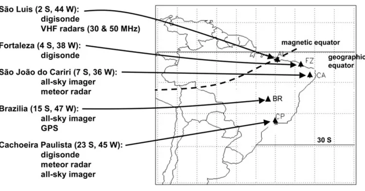
po-Fig. 2. Measurement sites in Brazil employed for the SpreadFExmeasurement campaigns. GPS receivers weremuchmore widely distributed, with ∼25 sites available for SpreadFEx.
Table 1. Instrumentation at the fixed INPE and temporary SpreadFExmeasurements sites employed for our experiment. GPS were also available at ∼20 other locations in Brazil.
Site Geogr. Magnetic Airglow VHF Meteor Digisonde GPS
latitude latitude radars radars
S˜ao Luis 2.6 S 1.5 S X X X
Fortaleza 3.9 S 5 S X X
Cariri 7.4 S 8 S X X X
Fazenda Isabel 15 S 9 S X X
Cach. Paulista 22.7 S 17 S X X X X
rary optical and GPSmeasurements weremade at Fazenda Isabel north of Brasilia and several nearby sites. Specif-ically, VHF radars at S˜ao Luis defined ESF altitudes and plasma bubble structures at themagnetic equator (de Paula and Hysell, 2004), meteor radars defined MLT winds at Cariri and Cachoeira Paulista (Batista et al., 2004; Buriti
et al., 2007), digisondes defined electron densities at sev-eral dip latitudes (Batista and Abdu, 2004), airglow cameras defined both GW structures at MLT altitudes and plasma bubble structures at higher altitudes in the thermosphere at several locations south of themagnetic equator in order to assess the spatial and temporal variability of these processes (Medeiroset al., 2004), and GPS sensors were employed to attempt to define the spatial and temporal variations in elec-tron densities (Lanyi and Roth, 1988). The instrument lo-cations and their relation to themagnetic equator are shown in Fig. 2 and listed in Table 1.
4.
Initial Results from SpreadFEx
4.1 Convection, GW sources and propagation
4.1.1 GOES 12 indications of deep convection GOES 12 visible, IR, and water vapormeasurements over Brazil (at 1-, 4-, and 8-kmresolutions, respectively) pro-vided the best way to quantify the locations, scales, and intensities of deep convection leading to GW generation and propagation to higher altitudes during SpreadFEx. Cold cloud-top temperatures indicate deep convection, and tem -poral variations between successive images provide an in-dication of updraft intensities and durations. These data are
being employed to estimate the spatial and temporal scales of convective plumes that are assumed to launch GWs prop-agating into the MLT and to higher altitudes. An example of the GOES 12 IR data showing deep convection, color-coded to highlight the coldest convective plumes, is shown for ref-erence in Fig. 3. This image shows a number of regions of active, deep convection. Five exhibit extensive cold tem -peratures, assumed to be the largest andmostmature con-vection, and themajor sources of GWs at this time. These occur near (2◦S, 68.5◦W), (2.5◦S, 67◦W), (6◦S, 62◦W), (8.5◦S, 62◦W), and (10◦S, 50.5◦W). Brasilia is at (15◦S, 47◦W), our temporary optical site was∼100 kmnorth, and the dip equator is shown for reference. There are also a series of smaller cells having cold cloud tops, but smaller spatial scales, a number of which would also be actively exciting additional GWs. The largest and deepest convec-tion is themost efficient source of GWs that penetrate to the highest altitudes, but the horizontal extent of the cloud top IR signatures often overestimates convective plume widths due to their generation of cirrus cloud shields as theym a-ture. Indeed, recent high-resolution numerical studies by Laneet al.(2003) and Lane and Sharman (2006) show that such large-scale convection is oftenmodulated by sm aller-scale∼5-kmplumes.
Fig. 3. GOES 12 convection observed in the IR channel at 20:54 UT on 24 October 2005. Cloud top temperatures are color coded, with solid (dashed) contours showing eastward (westward) GWmomentumfluxes predicted at 21:55 (blue) and 22:15 (red) UT at 200 km. The dominant GW propagation at 200 kmwas eastward at this altitude due to filtering of GWs by strong westward winds at lower altitudes. Our temporary optical site for SpreadFEx was∼100 kmnorth of Brasilia (shown with the yellow square).
Fig. 4. Zonal (left) andmeridional (center) wind and temperature (right) profiles at (47.6◦W, 14.75◦S) and 21:45 UT used for ray tracing GWs arising fromthe deep convective plumes observed in Fig. 3. The profiles were defined by balloon soundings below 30 km,meteor radar observations between 80 and 100 km, and a TIME GCM simulation initialized with the NCEP reanalysis data for this same period from35 to 70 kmand from110 to 350 km, with linear interpolation elsewhere.
and (5, 5, 5) kmfor the 3rd and 5th plumes listed above. Assumed updraft velocities for the five were 30, 30, 35, 30, and 15 ms−1, respectively. GWs assumed to arise from these plumes were ray traced froman assumed source al-titude of 14 kmupward through the zonal andmeridional wind fields and a temperature field defined in the follow-ingmanner. Balloon data were used to specify these fields fromthe surface to 30 km, meteor radar data fromCariri were used to define the low-frequency wind field between 80 and 110 km, and data froma therm osphere-ionosphere-mesosphere-electrodynamics (TIME) general circulation model (GCM) simulation, initialized with National Center for Environmental Prediction (NCEP) reanalysis data for this interval, were used to define the large-scale wind and temperature fields between 35 and 80 km, and again be-tween 110 and 350 km. The resulting wind and temperature profiles used for this purpose are shown at (45◦W, 10◦S) in Fig. 4. There is, however, considerable variability in the
wind field, and the GWs that survive to the highest altitudes are thus very sensitive to their source scales and locations. The resulting GWs were ray traced using themethodology of Vadas and Fritts (2004) and incorporated viscous dissi-pation at higher altitudes to assess maximum penetration altitudes (Vadas and Fritts, 2005).
wave-Fig. 5. Keograms prepared fromeast-west slices of 6300 ˚A (top) and OH (bottom) airglow emissions obtained at Brasilia (left) and Cariri (right) on 1 October 2005. Note thatmovement of structures in both emissions is generally eastward, but is faster and at∼100 to 500-kmzonal wavelengths in the TI and slower and at∼20 to 400-kmzonal wavelengths in the MLT
lengths (∼115±70 km) and occurring at larger distances fromthe convective sources. The earlier response is com -posed largely of westward-propagating GWs having nega-tive zonalmomentumfluxes (dashed contours), while the later response has preferentially southeastward propagation and positive zonalmomentumfluxes (solid contours). In all cases, the dominant responses at the higher altitudes are largely dictated by turning levels due to strong winds op-posite to GW propagation in the LT. At all times, however, GWs having high phase speeds are found to propagate in a range of directions, depending on the local winds.
Manymore GWs succeeded in penetrating from convec-tive sources into the MLT, and many of these were easily seen in the various airglow emissionsmeasured at our three SpreadFEx opticalmeasurement sites. These sites were typ-ically east of themajor convection, so the predominant east-ward propagation appears to be consistent with primarily convective sources. Examples of GW propagation in the east-west plane are shown with Keograms of OH airglow brightness fromBrasilia and Cariri in the lower panels of Fig. 5. Horizontal wavelengths were typically in the range
∼20 to 400 km, with the largest brightness variations oc-curring at intermediate scales of ∼50 to 200 km. While not displayed here, ray tracing of GWs having these hori-zontal scales, but lower frequencies than those penetrating into the TI, suggest largely eastward propagation and typ-ical propagation times of several hours fromtheir convec-tive sources to the MLT. These results are generally consis-tent with the scales and largely eastward propagation seen in Fig. 5. Based on these observations and the accom pa-nying ray tracing, wemust be careful in attempting to link GWs in the MLT with plasma instabilities and bubbles at higher altitudes, as what dominates the airglow brightness modulationsmay not fully characterize the GWs that sur-vive to 200 kmand above. More quantitative and complete
assessments of GW sources, generation, and spatial scales attaining MLT and higher altitudes are provided by Taylor
et al.(2008), Takahashiet al.(2008), Vadas et al.(2008), Vadas and Fritts (2008), Fritts and Vadas (2008), and Fritts
et al.(2008b) in our SpreadFEx special issue.
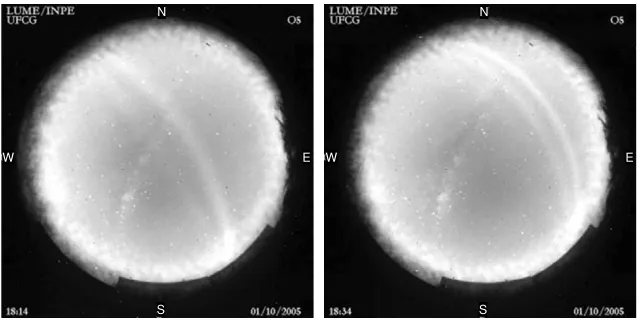
4.1.3 Bores in the MLT While not a central focus of the SpreadFExmeasurement campaigns, our airglow, radar, and related satellitemeasurements also provided sensitiv-ity tomesospheric bores occurring at MLT altitudes and to the wind and temperature fields in which they occurred. As bores are believed to be excited by GW instabilities, dis-sipation, and/ormean-flow interactions, their study repre-sents an interesting extension of our campaign objectives and specific GW studies, and it benefits significantly from our comprehensive SpreadFEx data set. One example of a bore seen at Cariri on 1 October is shown in Fig. 6 at two times separated by 20 min. This bore structure wasmost visible in the OI 5577 ˚A emission, propagated towards the NE, and had an initial wavelength that appeared to shorten and a number of crests that appeared to increase over the 20-min interval displayed. Analysis of this event suggests a complex ducting structure (Fechineet al., 2008) and helped motivate our initialmodeling studies of bore excitation and evolution in thermal and Doppler ducts.
Bore structures, evolutions, and excitation have been studied previously by Dewan and Picard (1998, 2001), Seyler (2005), Fechine et al.(2005), and Medeiros et al.
E
W W E
S N
S N
Fig. 6. A bore seen in OI 5577 ˚A emissions at Cariri on 1 October 2005 at times of 18:14 and 18:34 LT. The bore was less distinct in OH emissions, propagated towards the NE (upper right), and exhibited dispersion and an increasing number of wave crests in only 20min.
Fig. 7. Potential temperature and velocity profiles leading to ducting and enabling bore development and propagation (top). A sharp increase in potential temperature yields a localmaximumin buoyancy frequency squared,N2(z); the profiles at top right show displaced thermal and Doppler
ducts, which often accompanymean and low-frequency GW structures in the MLT. Lower panels show perturbation potential temperature fields exhibiting responses to horizontal Gaussian impulses for overlapping thermal and Doppler ducts when they overlapmore fully (middle) and to a smaller degree (bottom). Shown areN2and velocity profiles (solid and dashed, respectively), with a peakN2∼28 and 40 times the background (top
and bottom, respectively), a backgroundN=0.01047 s−1(a buoyancy period of 10min), thermal ducts of 8 and 3 kmFWHM (top and bottom),
Doppler ducts of 5 kmFWHM (both), and a velocitymaximumof∼100ms−1. The Gaussian horizontal impulse had amaximumof∼8ms−1and
250
Fig. 8. Digisondemeasurements at S˜ao Luis for 24 to 27 October 2005 (upper panel) and expanded versions of these data (from1800 to 0300 UT) for S˜ao Luis (lower left) and Fortaleza (lower right) for the first two of these nights. Inferred vertical velocities are shown on the bottomof the displays at S˜ao Luis for each night.
accompanying both thermal and Doppler ducts, we show two responses arising for sech2(z/h)Doppler and thermal ducts of different depths and displaced by half the FWHM of the Doppler duct in the vertical in themiddle and lower panels of Fig. 7. In these examples, we assumed a FWHM of the Doppler duct of 5 km, a Doppler duct jetmaximum of∼100ms−1, thermal duct FWHM of 8 and 3 km(top and
bottomimages in Fig. 8), a backgroundN =0.01047 s−1 (a buoyancy period of 10min) in both cases, and thermal duct maxima of N = 0.056 and 0.066 s−1, respectively. Both ducting environments were excited with a 2D horizon-tal Gaussian impulse ofmaximumvelocity∼8ms−1 and
FWHM of 5 kmcentered at the thermal duct.
For the broad thermal duct (middle panels of Fig. 7), there are two distinct ducted features, one occurring som e-what below the thermal duct propagating to the left and a second somewhat above the thermal duct propagating to the right. Each feature exhibits a largely anti-symmetric response in the temperature (and vertical velocity) field be-cause of the symmetric horizontal forcing and normal dis-persion, with the larger wavelengths having larger phase and group velocities than the smaller wavelengths. The larger and smaller wavelengths within each response are also centered at somewhat different altitudes. This is be-cause themean velocity varies across the thermal duct, and smaller-scalemotions having smaller phase speeds aremore influenced bymean winds and tend to occur nearer them
ax-imum velocity in their direction of propagation. In fact, the larger wavelength ducts are definedmore by the ther-mal structure, and the smaller wavelength ducts are defined more by the wind structure.
The lower panels in Fig. 7 shows the response when the thermal duct is both narrower (3 rather than 8 km) and stronger (a peak N2 ∼ 40 times, rather than ∼28
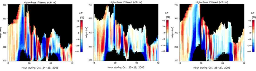
Fig. 9. Electron density fluctuations computed fromthe digisonde data for all three nights from1800 to 1200 UT. Note the large electron density fluctuations (up to∼40%), with oscillation periods of∼20min to 2 hr and apparent downward phase progressions at altitudes of∼280 kmand below. Note that largeKpvalues (∼4) occurred only on 25 October, with smaller values the following days.
4.2 Electron densities, TEC, and GWs in theFlayer We now turn to an overview of the observational evi-dence of possible neutral and plasma coupling at the bot-tomside F layer obtained during the SpreadFExm easure-ment campaigns. Digisondemeasurements at S˜ao Luis for 24 to 27 October 2005 are shown for reference in the up-per panel of Fig. 8. Expanded versions of these data (18 to 03 UT), and the corresponding data fromFortaleza, are shown for the first two of these nights (24/25 and 25/26 Oc-tober) in themiddle and lower panels, respectively. Elec-tron density fluctuations computed fromthe digisonde data fromS˜ao Luis for all three nights from1800 to 1200 UT are shown in Fig. 9. These perturbations appear larger than often observed elsewhere, but are indicative of the potential for large plasma density perturbations in theFlayer, though the specific roles of these perturbations in generating ESF and plasma bubbles are unclear at this time.
Each night exhibits the expected rise in theF layer ac-companying the PRE and a series of oscillations there-after having large amplitudes and apparent vertical dis-placements. Observed periods range from∼20min to 2 hr, with the largest electron density fluctuations (∼40%) oc-curring at the longer periods. Also seen are apparent down-ward phase progressions, especially at altitudes of∼280 km and below. These aremost apparent in the electron density fluctuations at the longer periods from∼00 to 04 UT for each day shown in Fig. 9. There are also several regions in each panel where opposite phases of the perturbation over-lap each other. This provides some indication of apparent GW vertical wavelengths. More quantitative estimates of GW amplitudes, scales, and likely propagation conditions inferred fromthese data are discussed in Section 5 below.
Prompt penetration electric fields have been suggested to lead to strong uplift of the F layer (Abduet al., 2003; Huanget al., 2004) and are expected to occur on a global scale (Kelley, 1989). Substorms may likewise contribute significant short-termperturbations at equatorial latitudes. Such effects are expected to be more pronounced under enhanced high latitude convection conditions, so we dis-play the Kp index during September and October 2005 in
Fig. 10. These data reveal significant Kp (∼4 from00 to
12 UT) the evening of 24/25 October, but with substantially smaller values of∼2 the next two nights. The Dst index,
which is available at significantly higher temporal
resolu-Fig. 10. Kpindex during September and October 2005. Tabular data yield
mean values of 1, 3.5, 2.5, and<2 for 24 to 27 October, respectively, averaged in UT.
tion, was likewise relatively quiescent, with mean values for 24 to 27 October of+1,−20,−21, and−15, with peak negative values of−39,−33, and−23 the last three days. ACE/MAG magnetic fields during these days were sim i-larly weak to moderate. Thus, apart fromthe evening of 24/25 October, with a mean Kp ∼ 4 and a mean Dst of
−20 nT, there is little evidence that there were significant geomagnetic influences. And even on this night, Dst
val-ues were substantially smaller than−100 nT, and are thus relatively geo-magnetically quiet.
Evidence of GWs at even higher altitudes is obtained fromGPS estimates of the temporal derivative of integrated or total electron content (IEC or TEC), assumed to be rep-resentative of changes at the altitudes of maximum elec-tron density, or sub-ionospheric point (SIP),∼300–400 km, by the use of various GPS receivers in Brazil. Examples of such information as derived from data obtained with the GPS receiver at Fortaleza on 24 October are shown in Fig. 11 which suggest typical GW periods at these altitudes of∼15 to 60min. The various satellites viewed by the re-ceiver during these times indicate similar temporal varia-tions at the same times, suggesting spatial coherence among the various “piercing points” of the ionosphere. For refer-ence, the vertical dashed red line in Fig. 11 indicates the anticipated start time for plasma bubble initiation (Wood-man and LaHoz, 1976), suggesting that the d(TEC)/dt
possi-24 Oct. 2005 (UT)
18 19
20
21 22
Fig. 11. Time series ofd(TEC)/dtfor eight GPS satellite traverses observed fromFortaleza during 24/25 October 2005 and coincident with the left perturbation electron density plot in Fig. 9. Note thatmost oscillations have apparent periods of∼20min to 1 hr and that oscillations are apparent well before spreadFonset, shown approximately by the dashed red line.
ble spatial variations accompanying slow satellitemotion. Nevertheless, they demonstrate fairly persuasively that GW perturbations in electron density also extend to higher al-titudes than implied unambiguously by the digisonde elec-tron densities.
To increase the potential for the detection of GWs and small-scale plasma structures in the ionosphere during SpreadFEx, five temporary GPS stations with an approx-imate spacing of 50 km between sites were also installed near the imager site in central Brazil at Fazenda Isabel, S˜ao Jo˜ao de Alianc¸a (FAZ1), Parque Nacional, Alto Paraiso (ALPA), Ibama, Alvorado do Norte (ALVO), Flores de Goias (FLOR), and Teresina de Goias (TERE). The loca-tions of each of these systems, along with permanent sites at Brasilia (BRAZ), Montes Ciaros (MCLA), and Uberlan-dia (UBER) from the Rede Brasileira de Monitoramento Cont´ınuo (RBMC) GPS network surrounding the tem po-rary GPS stations, are listed in Table 2. For these sys-tems, the integrated electron content (IEC) was calculated fromdual-frequency carrier phase observations (Lanyi and Roth, 1988; Hofmann-Wellenhof, 1994; Calais and Min-ster, 1998), with a 4th-order polynomial removed fromeach IEC time series to remove the effects of the diurnal variation in electron content. Array processing techniques developed to detect propagating disturbances in dual-frequency GPS time series (Calaiset al., 2003) are currently being used to
Table 2. Locations of the GPS sites in central Brazil employed for SpreadFEx.
Name Latitude Longitude
ALPA −14.073832 −47.788579
ALVO −14.406658 −46.506171
FAZ1 −14.665781 −47.602838
FLOR −14.49657 −47.034927
TERE −13.696128 −47.264411
BRAZ −15.93 −47.86
MCLA −16.71 −43.86
UBER −18.89 −48.31
characterize signals observed by this small array.
a)
b)
c)
d)
Fig. 12. (a) Detrended IEC time series for satellite PRN28 recorded at stations ALPA, TERE, FAZ1. Two troughs are seen at about 00:45 UTC and 01:30 UTC on 2 Oct 2005. (b) Detrended IEC time series for satellite PRN8. (c) Detrended IEC time series for satellite PRN4. (d) Map showing the traces of the subionospheric points for each satellite, with traces fromPRN4 furthest west, PRN8 in the center, and PRN 28 furthest east. Low amplitude of IEC in the detrended signal is shown in blue color. The perturbation is assumed to propagate perpendicular to the line spanned by the simultaneous troughs at ALPA and FAZ1 reaching TERE at a later time. Approximate propagation speeds are shown that have been derived from
data fromeach satellite. The location of the three GPS sites is indicated with red stars.
Assuming a disturbance propagating perpendicular to a line through ALPA and FAZ1 that reached the SIP fromTERE at a later time, a propagation speed of∼80ms−1in a
di-rection roughly ENE was inferred. Similarly, for PRN8 the propagation direction was approximately eastward at
∼101 m s−1, while traces from PRN4 showed eastward propagation at∼119ms−1. Indeed, the inferred propaga-tion direcpropaga-tions and speeds, as well as their variapropaga-tions with longitude and decreases with time, agree with similar es-timates using airglow imagers (see Fig. 5). Future analy-sis will attempt to estimate verticalmotions by combining SpreadFEx GPS and airglow data.
4.3 Spread F and plasma bubble occurrence, struc-ture, and correlations
The evolution of the bottomsideFlayer into plasma bub-bles extending to higher altitudes is illustrated in Fig. 13 with VHF radar RTI plots at S˜ao Luis for the nights of 24/25 and 25/26 October 2005. These data correspond to the first two nights of digisonde data and electron density fluctua-tions shown in Figs. 8 and 9. The RTI plots indicate the presence of ESF at the bottomsideFlayer beginning as low as∼230 to 250 kminmost cases, with apparent backscatter
also occurring on 24/25 October as low as∼200 km begin-ning just before 00 UT. Plasma bubbles appear not to be initiated until the bottomsideFlayer is elevated to altitudes of∼250 to 300 km. Wemust be careful in our interpreta-tion of these data, however, as plumes that are first observed at higher altitudes were necessarily seeded at earlier times to the west of S˜ao Luis.
Closer examination of Fig. 13 (top panel) suggests that ESF and RTI lead to bubble generation accompanying the strong upward motions of the bottomside F layer at
∼22 UT and just before 00 UT on 24/25 October that are also seen in the digisonde data of electron density fluctua-tions in Figs. 8 and 9. The periodicity of the plasma bub-ble generation appears consistent with the lower-frequency modulations (∼2-hr periods) in these other data sets that were suggested to indicate possible GW influences below
Fig. 13. SpreadFand plasma bubbles observed on 24/25 (top) and 25/26 October (bottom) by the VHF radar at S˜ao Luis during the SpreadFEx
measurement campaign. The plume occurrence on both days follows closely the uplifted bottomsideFlayer seen in Figs. 8 and 9 and exhibits a similar periodicity.
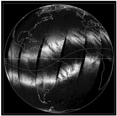
Fig. 14. TIMED/GUVI 1356 ˚A emissions on successive orbits dur-ing the SpreadFEx campaign. Dark bands are field-aligned and verti-cally-integrated plasma depletions.
a challenge in interpreting our ground-based plasma bubble measurements, as the RTI plots display amixture of spatial structures and temporal variability.
Shorter period fluctuations (∼30 min) also seen in the
electron density data did not obviouslymake distinct con-tributions to plasma bubble seeding or spatial structure. To the extent that the∼2-hr oscillations at lower altitudes are indicative of GW perturbations, these data suggest that neu-tral atmosphere GWmotionsmay have played an important role in the seeding process. The same periodicities were also present at the bottomside F layer on 25/26 October (Figs. 8, 9, and 13, bottom, center, and bottompanels), and the longer periods (∼2 hr) again appear to correlate well with the vertical plasmamotion at these altitudes. In this case, shorter periods weremore prevalent in the digisonde and electron density data andmay have played a larger role in seeding the apparentlymore complex bubble structures at higher altitudes. Again, however, it appears difficult to establish a clear correlation between fluctuations at the bot-tomsideF layer and the plasma bubbles observed at higher altitudes after the initial bubble occurrence because the later bubbles were already fully developed when observed over S˜ao Luis. The potential for GWs present at the bottom -sideF layer to contribute to plasma instability seeding and growth rates is explored in greater detail below.
Fig. 15. Vertical cross-sections (left) of plasma depletions at 19◦S (top) and 12◦S (bottom) fromtomographic inversions of GUVI 1356 ˚A emissions (left) and corresponding 6300 ˚A emissions at Cariri (right) for 1 and 2 October (days 274 and 275), respectively. Note that the images were not coincident in longitude on day 274, but were on day 275.
Fig. 5, provide information on spatial scales and drift speeds. These suggest typical plume separations of∼100 to 500 km, at least at the altitudes that contributemost to plasma depletions, will play an important role in ourmore quantitative analyses to follow. Additional information on plasma bubble geometries and evolutions can be obtained by interferometric analysis of the VHF radar data (Hysell, 1996), but these results will likewise await our Spread-FEx special issue. Finally, data fromthe GUVI instrument aboard the TIMED satellite will be seen below to yield a dramatic enhancement of our ability to quantify plasma bubble structures via tomographic inversions of 1356 ˚A emissions at the times of these overpasses.
4.4 Plasma bubble structures inferred from space The GUVI instrument aboard the TIMED satellite pro-vides another valuable data set for plasma bubble studies, and there were several overpasses that were coincident in space and time with some of our SpreadFExmeasurements. The primarymeasure of bubble structures by GUVI is via the 1356 ˚A emissions, which show significant line-of-sight depletions when viewing bubbles near nadir. An exam -ple of the bubbles seen by GUVI over S. America during our SpreadFExmeasurements is shown in Fig. 14. These data afford another opportunity to correlate bubble struc-tures with 6300 ˚A airglow images and VHF radar RTI plots
in defining bubble scales andmorphology.
Evenmore exciting is the ability to performtomographic inversions with the GUVI data because the satellite m o-tion and GUVI viewing have components normal to the magnetic field over Brazil. This allows extraction of elec-tron density measurements in a plane normal to the field lines having horizontal and vertical resolution of∼40 and 20 km, respectively. This allows for unprecedented reso-lution of the spatial scales of individual bubbles andmuch more quantitative comparisons with our SpreadFEx correl-ative data than would otherwise be possible. Two examples of these data from1 and 2 October and the corresponding 6300 ˚A airglow images fromCariri viewing the same bub-ble structures are shown in Fig. 15. While we did not per-forman extensive analysis of these correlative data prior to writing this paper, this is the focus of the effort by Kam al-abadiet al.(2008) in the SpeadFEx special issue.
5.
Potential Neutral Atmosphere Contributions to
ESF, RTI, and Plasma Bubble Seeding
o-over Brazil at 21 (dashed), 00 (solid), and 03 UT (dash-dotted) for a TIME GCMmodel run spanning the SpreadFEx campaign period and initialized with the global NCEP reanalysis for this period.
spheremotions to plasma instabilities accompanying neu-tral wave perturbations occurring at F layer altitudes. An assessment of possible GW influences at lower altitudes that map electric field or other perturbations to higher altitudes ismore complex and beyond the scope of this summary of first SpreadFEx results. Formore complete discussions of related SpreadFEx analyses, we refer the interested reader to Frittset al.(2008a, b), Abduet al.(2008), Kheraniet al.
(2008), and other papers in the SpreadFEx special issue. 5.1 Tidal influences at the bottomsideFlayer
Amajor contributor to TI structure that appears to have obvious relevance to the preconditioning arguments of Kudekiet al.(2007) is the neutral atmosphere tidal structure that penetrates to high altitudes, and is generated in situ, at equatorial latitudes. Themigrating tides are expected to comprise the dominantmotion field atFlayer altitudes, and their temporal behavior described by the TIME GCM ap-pears to make a clear contribution to the potential plasma instability processes envisioned by these authors (we note, however, that the TIME GCM tidal structures at F layer altitudes have yet to be validated, so their detailed am pli-tude and phase structures should be considered to be only suggestive at this time). Zonal tidal winds on 25/26 Oc-tober 2005 over the dip equator in Brazil at 21, 00, and 03 UT for amodel run spanning the SpreadFEx campaign period are shown in Fig. 16. These profiles suggest that zonal winds are small or negative (westward) at∼21 UT and swing sharply positive (eastward) thereafter at Flayer altitudes, which appears to correlate well with onset times for plasma bubbles noted by previous authors. If the de-pendence of ESF initial instability is indeed a strong func-tion of eastward winds, as argued by Kudekiet al.(2007), then it seems likely that tidal winds will play a very large role in determining when strong instability is possible, or at the least, inmodulating instability growth rates. Because tidal structures exhibit significant amplitude variability at lower altitudes, due both to variable forcing in the lower at-mosphere andmodulation of processes coupling to higher altitudes, they are also expected to impose this variability on ESF, RTI, and plasma bubble occurrence statistics atF
ment envisioned by Hysellet al.(2004) shown in Fig. 17. This schematic, and the arguments by Kudekiet al.(2007), suggest that instability will be favored for perturbations that enhance both electron density gradients and neutral-minus-plasma zonal motions (Un −Up) in regions where
the plasma has been elevated. This is the lower left quad-rant of the clockwise circular plasma motion depicted in Fig. 17, where the plasmamotion opposes the neutralm o-tion and induces risingmotion westward and above, which increases the perturbation displacements. As we will see below, GWs can enhance eastwardmotions accompanying either upward or downwardmotions, but enhanced neutral and plasma density gradients always accompany downward neutralmotions.
Considering first the neutral GW perturbations implied by a given fractional electron density gradient, we assume mean neutral and electron density profiles of the form
ρ(z)=ρe−z/H (3)
and
ρe(z)=ρeez/He, (4)
where H and He are the respective (positive) neutral and
electron density scale heights. We also assume GW veloc-ity, pressure, potential temperature, and neutral density per-turbations of the form
(u, v, w, p/p, θ/θ, ρ/ρ)
∼exp [i(kx+l y+mz−ωt)+z/2H],(5)
where primes denote perturbations andk=(k,l,m)is the GW wavenumber vector. Assuming that the plasmamoves with the GW perturbation wind field and that there are no chemical or electrodynamic processes that also impact plasma densities, the electron (or ion) continuity equation,
dρe/dt=0,may be written as
ρ
e/ρe=ku/ω+lv/ω+mw/ω−iw/ωHe. (6)
Employing the energy conservation and continuity equa-tions (Fritts and Alexander, 2003)
iω θ/θ =N2/gw (7)
and
iω ρ/ρ=i ku+ilv+(i m−1/2H)w. (8)
Assuming thatmotions are approximately hydrostatic such thatθ/θ ≈ −ρ/ρ and employing the relation N2H/g+
Finally, the GW polarization relations (Fritts and Alexan-der, 2003) yield relations for vertical and horizontal pertur-bation velocities in terms of fractional densities
w∼gω/N2ρ/ρ, (10) In the above,uhandware the horizontal and vertical GW perturbation velocities, ω = kh(c −Un) is the GW
in-trinsic frequency, kh = (k2+l2)1/2 = 2π/λh andm =
2π/λzare the GW horizontal and vertical wavenumbers,c
andUn are the GW horizontal phase speed and the
neu-tral mean wind in the direction of propagation (assumed zonal in the discussion of plasma instabilities above), λh
andλzare the GW horizontal and vertical wavelengths, and β ∼ (1−ω2/N2)1/2 ∼ 1 for hydrostatic and small-scale
GWs. With our degree of approximation, Eq. (10) is accu-rate for all GWs in the TI, whereasβ ∼1 in Eq. (11) only whenλ2
h 16π2H2andω2 N2. These are reasonable
assumptions at lower altitudes, but they are less accurate where GW vertical wavelengths exceed∼100 kmand in-trinsic frequencies exceedω∼N/3, as we expect to occur in response to increasing kinematic viscosity and thermal diffusivity in the TI (Vadas and Fritts, 2005, 2006; Vadas, 2007; Fritts and Vadas, 2008). Whenω > N/1.4 and GW scales increase,β < 1/2 and approximations appropriate for the lower atmosphere lead to overestimates ofuhbased on densitymeasurements. We again note that we have con-sidered only advective effects in the above discussion, and have specifically neglected chemical, electrodynamic, and magnetic influences on plasma densities hatmay be com -petitive. Thus, plasma perturbations will almost certainly be smaller than suggested by the above equations.
Under solarminimumconditions, thermospheric tem per-atures above∼200 kmare∼600 K and gradients are small, such that N ∼10−2 s−1and the buoyancy period is T
b ∼
10min. Thus we should expect typical GW intrinsic peri-ods ofTi=2π/ω∼30min (Vadas, 2007; Fritts and Vadas,
2008), and the GWs suggested by the electron density and TEC fluctuations discussed above are in the expected range. We also expect neutral and electron density scale heights of
H ∼ 15 to 20 kmand He ∼ 20 to 50 km, such that the
ratio of fractional electron to neutral density fluctuations is likely something less than(ρe/ρe0)/(ρ/ρ0)∼5 or smaller.
The 10 to 40% electron density fluctuations inferred from the digisonde data then imply horizontal and vertical GW perturbation velocities ofu ∼10 to 40ms−1andw∼3 to 10ms−1 (or larger, if electron density fluctuations are
under-estimated) ifmotions occurred at smaller scales and nominal intrinsic frequencies ofω ∼ N/3, with estimates foru ∼ 2 times smaller for higher frequencies and larger scales. Thus, the velocity perturbations of GWs believed to have been present in the bottomsideF layer during plasma bubble seeding during the SpreadFEx measurements ap-pear to have been sufficiently large to impact plasma in-stability growth rates if they existed in the relevant regions and induced the appropriate perturbations to the differen-tial plasma and neutral zonal velocities and/or the length scale (He) of the electron density gradient. As suggested
above, GWs also contribute to perturbations of themean electron density gradient andmay thus contribute tom od-ulation of plasma instability growth rates through both dif-ferential neutral and plasmamotions and enhanced electron density gradients.
5.3 GW impacts on plasma growth rates
We now consider the GW orientations and structures im -plied by our SpreadFExmeasurements and their possible contributions to plasma instabilities and growth rates, with a focus on direct influences at the bottomside Flayer. Our SpreadFEx airglow observations and our limited ray trac-ing of GWs fromconvective plumes to date imply a prefer-ence for approximately zonal GW propagation in the MLT, though thismay simply be a consequence of our SpreadFEx observations occurring generally to the east of themost in-tense convection. The TIME GCM simulation results em -ployed here imply strong zonal andmeridional tidal winds (and associated GW filtering) exhibiting significant spatial (in altitude and latitude) and temporal variability at the bot-tomsideF layer. However, the tendency for eastward tidal winds to arise in the early evening hours appears to be con-sistent with the needed orientation of neutral atmosphere perturbations potentially contributing to RTI seeding and plasma bubble generation. This also implies preferential westward GW propagation at these altitudes, though weaker winds at lower altitudes would allow more isotropic GW propagation.
Assuming first thatρerather thanρe/ρe0is constant with
altitude, because of the apparentmaxima of the latter be-tween∼250 and 300 kmand the apparent decrease above, we can express the local electron density gradient as (again assuming only advective effects)
maximumneutral and electron densities, respectively. Neutral zonal and vertical winds are shown with blue arrows, the black circle shows the expected plasmamotion (Hysellet al., 2004), and the pink region shows where neutral GWmotions oppose horizontal and vertical plasma
motions (contributing to polarization electric fields) and enhance the vertical electron density gradient, all of which enhance the expected plasma instability growth rates anticipated by Kudekiet al.(2007).
=ρe0
The ratio of perturbation to mean contributions is then
∼(ρ
e/ρe0)m He within the phase of the GW having the
largest positive gradient. For a GW with a vertical wave-length ofλz ∼100 km, which is consistent with apparent
vertical structure in the electron density fluctuations seen in Fig. 9 and with expectations of assessments of GW wave-length variations due to increasing kinematic viscosity in the TI (Vadas and Fritts, 2006; Vadas, 2007; Fritts and Vadas, 2008), this ratiomaximumis
ρ
e
ρe0
m He∼0.5 to 1 (13)
for the ranges of reasonable GW amplitudes, wavelengths, and plasma scale heights He anticipated at the bottomside
F layer.
We are now in a position to assess how the various GW perturbations of horizontal and vertical winds and plasma density gradientsmay impact the plasma growth rates dis-cussed above (with the above caveats about the neglect of chemical and electrodynamics effects). We begin by sum -marizing themean structure of the neutral thermosphere and ionosphere anticipated to yield significant plasma growth rates by Kudekiet al.(2007). These conditions are shown in the left panel of Fig. 18. The important features appear to be 1) an eastward neutral wind at higher altitudes (due largely to tidalmotions that only become significantly east-ward at the time of observed plasma bubble formation), 2) a westward plasmamotion partially decoupled fromthe neu-tralmotions at the bottomsideFlayer, and 3) a strong ver-tical plasma (and electron density) gradient at the same al-titudes. Considering GW influences on both neutral winds and electron density and plasma gradients, there are two possible GW orientations that imply different contributions to key terms in the instability growth rates. A GW having
withmaximumupward and downward displacements (blue and red dashed lines) corresponding to the regions ofm in-imumandmaximumelectron densities, respectively. Neu-tral GW wind perturbations (with zonal and vertical com -ponents anti-correlated) are shown with blue arrows, and the black circle shows the expected plasmamotion leading to instability growth in the westward and upward phase of plasmamotion (Hysellet al., 2004). The pink region shows where neutral GWmotions oppose horizontal plasmam o-tions (increasing the neutral-plasma velocity difference by up to ∼20%, thus amplifying polarization electric fields) and enhance the vertical electron density gradient, all of which enhance the expected plasma instability growth rates anticipated by Kudeki et al. (2007) in this region of the flow. Thus, we conclude that GW perturbations may have substantial influences on plasma instability growth in two ways: 1) they may significantly enhance plasma instabil-ity growth rates through perturbations of the neutral and plasma quantities upon which the growth rates depend and 2) they may induce “seed” perturbations at suitable spatial scales, allowing more rapid attainment of finite-amplitude perturbations extending to higher altitudes. Finally, the westward intrinsic phase speed of the hypothesized GW of
(c−Un)∼Nλz/2π∼160ms−1implies westward
propa-gation, a phasemotion close to that of the westward plasma drift, and hence amuch longer time for coherent perturba-tions to act on the underlying plasma than suggested by the much higher GW intrinsic frequency. Similar arguments can bemade about the potential effects of GWs propagat-ing eastward or superpositions of GWs havpropagat-ing various prop-agation directions (see Fritts et al., 2008b). These influ-ences will vary with the relative contributions of the GW to horizontal and vertical velocity and plasma density gra-dient fluctuations. In either case, it appears to us that it is likely that large-amplitude GWs at the bottomsideF layer contribute to growth of the plasma instabilities and plasma bubbles extending tomuch higher altitudes.
6.
Summary of Initial SpreadFEx Results
at this stage, and refer readers to our forthcoming Spread-FEx special issue ofAnnales Geophysicae formore com -prehensive analyses. Current conclusions include:
a) deep convection appears to be a significant and viable source of GWs penetrating into the MLT and to the bottomsideFlayer, depending on GW scales, frequen-cies, and propagation directions;
b) GWs spanning a wide range of scales and frequencies can reach the MLT, but only GWs having large scales and high frequencies can reach higher altitudes; c) GWs arising fromconvection are strongly influenced
by lower atmospheric and MLT winds that dictate which GW frequencies, scales, and propagation direc-tions allow penetration to the bottomside F layer and above;
d) digisonde electron densities suggest GWs having downward phasemotions (upward propagation), peri-ods of∼20min to 2 hr, and significant electron den-sity perturbations at the bottomsideF layer, with cor-responding implied neutral density and wind perturba-tions;
e) GPS data suggest GWs of similar periods extending to even higher altitudes before and after plasma bubble occurrence;
f) smaller-scale GWs and wave-mean flow interactions appear to excite bores in the MLT that exhibit a variety of dispersive and nonlinear responses;
g) VHF radar and digisonde data suggest a connection be-tween rising plasmamotions, decreasing electron den-sities, increasing plasma gradients, and plasma bubble initiation;
h) VHF radar, digisonde, GPS, airglow, and GUVI data suggest an ability to quantify plasma perturbations in altitude, longitude, and time; however, it remains un-clear how these perturbations are related to plasma bubble generation;
i) neutral zonal tidal winds appear to play an im por-tant role in enabling spreadFseeding, given the tran-sition fromwestward to eastward neutral motions at
∼250 kmand above in the early evening hours; j) themultiple correlative data sets collected during the
SpreadFEx campaigns are among the most com pre-hensive available, and will likely enablemore quantita-tive conclusions upon completion of our various anal-yses;
k) our initial results lead us to conclude that GWsmay have sufficient perturbation amplitudes and impacts on instability growth rate at the bottomside F layer that their potential role in ESF and plasma bubble seeding should not be discounted;
and
l) it remains to be quantified fully how the GW neu-tral and electron density perturbations identified in our SpreadFEx experiment affect the generation of ESF and plasma bubbles extending to higher altitudes.
Acknowledgments. The SpreadFEx field programand data anal-ysis were supported by NASA under contracts NNH04CC67C and NAS5-02036. Relatedmodeling and theoretical activities were supported by NSF grants ATM-0314060 and ATM-0537311 and AFOSR contract FA9550–06-C-0129. We also thank M. R.
Haus-man and L. J. Nickisch for their assistance in analyzing GPS data fromFortaleza and V. T. Rampinelli, E. Bataglin, J. Sempere, N. D. Cˆandido, and the S˜ao Jo˜ao d’Alianc¸a’s House of Representa-tives and S˜ao Jo˜ao d’Alianc¸a’s Mayor’s House for local support during the campaign. CPTEC-INPE provided assistance with the GOES 12 data analysis. Some of the authors also had partial sup-port fromConselho Nacional de Desenvolvimento Cietifico e Tec-nologico CNPq (Abdu, Sobral, de Paula, I. Batista, Takahashi, and Gobbi). Finally, we thank Wenbin Wang and two anonymous re-viewers for helpful comments on themanuscript.
References
Abdu, M. A., Outstanding problems in the equatrial ionosphere-thermosphere systemrelevant to spreadF,J. Atmos. Sol.-Terr. Phys., 63, 869, 2001.
Abdu, M. A., I. S. Batista, and J. H. A. Sobral, A new aspect ofmagnetic control of equatorial spreadF,J. Geophys. Res.,97, 14,897, 1992. Abdu, M. A., I. S. Batista, H. Takahashi, J. MacDougall, J. H.
So-bral, A. F. Medeiros, and N. B. Trivedi, Magnetospheric distur-bance induced equatorial plasma bubble development and dynamics: A case study in Brazilian sector,J. Geophys. Res.,108(A12), 1449, doi:10.1029/2002JA009721, 2003.
Abdu, M. A., E. A. Kherani, I. S. Batista, E. R. de Paula, and D. C. Fritts, An evaluation of the ESF/bubble irregularity growth conditions under gravity wave influences based on observational data fromthe SpreadFEx campaign,Ann. Geophys., SpreadFEx special issue, 2008 (submitted).
Aggson, T. L., N. C. Maynard, W. B. Hanson, and L. Saba Jack, Electric field observations of equatorial bubbles,J. Geophys. Res.,97, 2997, 1992.
Anderson, D. N., A. D. Richmond, B. B. Balsley, R. G. Roble, M. A. Biondi, and D. P. Sipler, In situ generation of gravity waves as a possible seedingmechanismfor equatorial spread-F,Geophys. Res. Lett.,9, 789–792, 1982.
Basu, B., On the linear theory of equatorial plasma instability: com pari-son of different descriptions,J. Geophys. Res.,107(A8), doi:10.1029/ 2001JA000317, 2002.
Batista, I. S. and M. A. Abdu, Ionospheric variability at Brazilian low and equatorial latitudes: comparison between observations and IRImodel,
Adv. Space Res.,34, 1894–1900, 2004.
Batista, P. P., B. R. Clemesha, A. S. Tokumoto, and L. M. Lima, Struc-ture of themean winds and tides in themeteor region over Cachoeira Paulista, Brazil (22.7◦S,45◦W) and its comparison withmodels,J. At-mos. Sol.-Terr. Phys.,66(6–9), 623–636, 2004.
Batista, I. S., M. A. Abdu, A. J. Carrasco, B. W. Reinisch, E. R. de Paula, and N. J. Schuch, Equatorial spreadFand sporadicE-layer connections during the Brazilian Conjugate Point Equatorial Experiment—COPEX,
J. Atmos. Sol.-Terr. Phys., 2008 (in press).
Buriti, R. A., W. K. Hocking, P. P. Batista, A. F. Medeiros, and B. R. Clemesha, Observations of equatorialmesospheric winds over Cariri (7.4 S) by ameteor radar and comparison with existingmodels,Ann. Geophys., 2007 (submitted).
Calais, E. and J. B. Minster, GPS, earthquakes, the ionosphere, and the Space Shuttle,Phys. Earth Planet. Inter.,105(3–4), 167–181, 1998. Calais, E., J. S. Haase, and J. B. Minster, Detection of ionospheric
pertur-bations using a dense GPS array in Southern California,Geophys. Res. Lett.,30(12), 2003.
de Paula, E. R. and D. L. Hysell, The S˜ao Luis 30 MHz coherent scatter ionospheric radar: systemdescription and initial results,Radio Sci.,39, RS1014, doi:10.1029/2003RS002914, 2004.
Dewan, E. M. and R. H. Picard, Mesospheric bores,J. Geophys. Res., 103(D6), 6295–6306, 1998.
Dewan, E. M. and R. H. Picard, On the origin ofmesospheric bores,J. Geophys. Res.,106(D3), 2921–2928, 10.1029/2000JD900697, 2001. Djuth, F. T., M. P. Sulzer, J. H. Elder, and V. B. Wickwar, High-resolution
studies of atmosphere-ionosphere coupling at Arecibo Observatory, Puerto Rico,Radio Sci.,32, 2321–2344, 1997.