R E S E A R C H
Open Access
A genetic algorithm-based job scheduling
model for big data analytics
Qinghua Lu
*, Shanshan Li, Weishan Zhang and Lei Zhang
Abstract
Big data analytics (BDA) applications are a new category of software applications that process large amounts of data using scalable parallel processing infrastructure to obtain hidden value. Hadoop is the most mature open-source big data analytics framework, which implements the MapReduce programming model to process big data with
MapReduce jobs. Big data analytics jobs are often continuous and not mutually separated. The existing work mainly focuses on executing jobs in sequence, which are often inefficient and consume high energy. In this paper, we propose a genetic algorithm-based job scheduling model for big data analytics applications to improve the efficiency of big data analytics. To implement the job scheduling model, we leverage an estimation module to predict the performance of clusters when executing analytics jobs. We have evaluated the proposed job scheduling model in terms of feasibility and accuracy.
Keywords: Big data, Hadoop, MapReduce, Job scheduling, Genetic algorithm
1 Introduction
Big data analytics (BDA) applications are a new cate-gory of software applications that process large amounts of data using scalable parallel processing infrastructure to obtain hidden value. Hadoop [1] is the most mature open-source big data analytics framework, which imple-ments the MapReduce programming model [2] proposed by Google in 2004 to process big data. Scalability is the most important feature of Hadoop, mainly because it can easily add compute nodes in the original cluster to analyze big data.
The performance of big data analytics application is related to the characteristics of jobs and the configuration of clusters, which have a direct impact on performance of big data analytics applications. When there are multiple jobs that need to be executed with diverse cluster con-figurations, the solution space of job scheduling is huge and manual job scheduling is inefficient and can hardly achieve the best performance.
Genetic algorithms (GAs) [3] are used to obtain opti-mized solutions from a number of candidates. GAs are inspired by an evolutionary theory: weak and unit species
*Correspondence: [email protected]
College of Computer and Communication Engineering, China University of Petroleum, Qingdao, China
are faced with extinction by natural selection and the strong ones have greater opportunity to pass their genes to future generations via reproduction [4]. Compared with other classic optimization methods, GAs have its specific advantages in terms of its broad applicability, ease of use, and global perspective [5]. GAs are particularly useful to one-objective and multiple-objective optimization prob-lems [6] that make one- or multi-objective attainment to the optimum.
The contribution of this work is mainly twofold. First, we propose an estimation module to predict the perfor-mance of Hadoop clusters when executing different big data analytics jobs, which can be used by GAs. Then, with the effective information which the estimation mod-ule provides, we present a genetic algorithm-based job scheduling model for geo-distributed data.
We evaluate the proposed solution using the data cen-ters and cluster nodes from the Amazon EC2 [7] platform. The experiment results show the proposed job scheduling model is effective and accurate.
The remainder of the paper is organized as follows: Section 2 describes the five basic stages of MapRe-duce data processing that can be utilized in the cal-culation of estimation module. Section 3 presents the genetic algorithm-based job scheduling model. Section 4 details the performance estimation module, which is used
by the algorithm for the calculation of time objective. Section 5 implements and evaluates the genetic algorithm. Section 6 covers the related work. Section 7 concludes the paper.
2 Related work
There have been numerous works devoted to Hadoop’s performance prediction. Berli´nska and Drozdowski [8] propose a mathematical model of MapReduce and ana-lyze MapReduce distributed computations as a divisible load scheduling problem. However, they do not consider the system constraints. There is also some work on opti-mizing MapReduce [9, 10]. Zaharia et al. [10] proposed a prediction model for sub-tasks of Hadoop job, rather than the entire job. Xu et al. [11] extracted character-istic values related to Hadoop performance and utilized machine learning methods to find the optimal value, with-out building performance models. Han et al. [12] pro-posed a Hadoop performance prediction model. However, it does not consider the data preparation phase of this thesis.
There are also some GA-based approaches proposed in job scheduling. Krishan Veer and Zahid [13] presents a design and eventual analysis of a scheduling strat-egy using GA that schedules the job with the objec-tive of minimizing the turnaround time of the job. The evaluation is simplified due to the limitations. In [14], the application of meta-heuristic for cloud task schedul-ing on Hadoop is investigated. A schedulschedul-ing algorithm using execution time, order of task arrival, and loca-tion of data (i.e., assign task to the node which con-tains the required data) to determine the best execution schedule is presented. But the performance prediction model is unintelligible, and the cost is not taken in consideration.
3 Background
Hadoop consists of the MapReduce algorithm and the Hadoop Distributed File System (HDFS) [15]. The Hadoop workflow includes five phases, which is illus-trated in Fig. 1.
• Prepare. The source data in the local disk is uploaded to HDFS in this phase. According to the predefined partition size of the data segmentation, source data are segmented in blocks first and then stored a copy to the data node in the pipeline way according to the network topology distance.
• Map. Each mapper reads data blocks from HDFS and generates key-value pair<k1,v1>of the input data. Then, it executes a user-defined map method which generates intermediate data<k2,v2>.
• Copy. It is also called shuffle. The intermediate data from the mapper nodes is passed to the appropriate
reducer based on the key. The process is from the completion of the first map wave to all intermediate data mapper outputs having been transferred to the reducer.
• Sort. This stage occurs before the reduce phase. The values of the output data from the map are sorted by the sort algorithm in accordance with the different keys and output the key-value pairs<k2,list(v2) >
for the reduce phase. All the values are sorted in list(v2).
• Reduce. In this phase, the user-defined reduce method are executed to generate the key-value pairs <k3,v3>as the final result.
This paper utilizes the performance module for the case of this paper to predict Hadoop data processing performance including the abovementioned five phases. After the time consumption characteristics have been pre-dicted, we can infer the cost of big data processing jobs, which depends on the characteristics of time consump-tion.
4 Design of the genetic algorithm-based job
scheduling model
4.1 Overall design of the GA-based approach
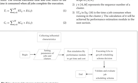
The working flow of the GA-based decision-making for job scheduling is shown in Fig. 2, and the overall decision-making process is as follows. First, the estimation module is used to model the clusters and jobs. Then, some simula-tions are conducted to collect job execution information, such as the time and cost array which shows all the time and cost taken by each job run on all clusters. After that, the time and cost information is used in certain frame-work where GAs give optimized solutions for the job scheduling schema.
For big data, we choose a certain cluster deployment way to process them. However, different processing jobs do not always have the same performance with the same cluster configuration, due to the job characteristics and one job also cannot obtain the consistent result with different clusters because of the cluster or Hadoop char-acteristics.
Fig. 1Traditional MapReduce workflow
We give a general mathematical description of the prob-lem and then create the appropriate objective optimiza-tion model based on genetic algorithms: take the data processing in a data center, for example, and assume that a data center has N optional clusters and M jobs to be executed. We use an integer vector to represent the ulti-mate job scheduling scheme,Si indicates that the jobiis
assigned to the clusterSi, where Si ∈[ 0,M]. So far, we
have achieved getting the job scheduling scheme which have the shortest overall execution time by genetic algo-rithm. The overall execution time and cost refers to the time it consumed when all jobs complete the execution.
Ti=
M
j=0STij×E(i,j) (1)
Ci=
M
j=0SCij×E(i,j) (2)
Here, we utilize Eqs. (18) and (19) to respectively represent the execution time and cost of all jobs assigned to one cluster, which are the objectives we considered in genetic algorithm. In order to facilitate the calculation of the overall execution time of job scheduling scheme, we addE(i,j)to indicate whether jobiis assigned to the clus-terj. The explanations of the symbols in the two equations are described one by one as follows:
1) i represents the sequence number of a job with the scope of[ 0,N].
2) j∈[ 0,M]represents the sequence number of a cluster.
3) STijin Eq. (18) is the time a job consumes when
running in the clusterj. The calculation of it will be achieved by performance estimation module in the next section.
4) SCij=Cij×STij×Nclusin Eq. (19) is to calculate the
cost of running a job in the clusterj , in whichCij
represents the cost of running a certain node per second andNclusis the number of nodes in clusterj .
5) When jobi is assigned to cluster j ,E(i,j)=1; otherwiseE(i,j)=0.
A chromosome corresponds to a unique solution in the solution space. GAs can typically make use of Booleans, real numbers, and integers to encode a chromosome [9]. The representation of chromosome in our case is using integer (starting from 0) sharing the idea of [10].
That is to say, we are using an integer vector V =
[V0,V1,,Vi,,Vp−1] (wherepis the number of decision variables, and in our case, it is 12: the number of jobs) to represent a solution which is a natural number and acts as a pointer to the sequence of the cluster to which the job is assigned to execute. For example, a chromosome [0, 6, 2, 8, 2, 4, 5, 9, 6, 1, 3, 7] represents that a solution chooses the first cluster whose sequence number is 0 to execute job 0 and chooses the eighth cluster for job 9, the eleventh cluster as the processing cluster of the third job, and so on. Based on the chosen allocation strategies, the GAs then decide its fitness using the objective Eqs. (1) and (2) introduced.
5 Performance estimation module of job
execution
5.1 Assumption
To achieve the genetic algorithm for job scheduling prob-lem, we need to input the source data of the two objec-tives: time and cost array. In this paper, we propose a performance estimation module which can predict the execution time and cost of data processing jobs, according to different characteristics. The paper makes the following assumptions for simplification:
• About the reduce wave, we use recommendations in [16] and assumes that the maximum number of reduce that can be executed simultaneously is 1. • We do not support speculative execution. That
means, we will not repeat map or reduce execution and select the faster as the final result, killing the slower one, for it proved to have little contribution to improve the overall execution time.
5.2 Total execution time overview
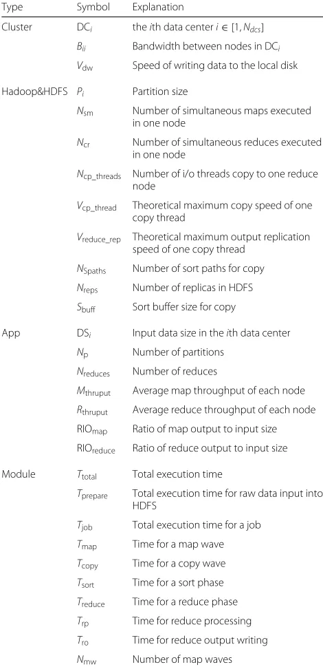
In this paper, performance-related parameters are divided into four categories: cluster, hadoop&HDFS, application, and obtained by module. The symbol and explanation of all parameters are listed in Table 1.
The overall data processing time contains two parts: one part is the preparation time of the source data and the other is the time to perform the data processing job.
Table 1Symbol and explanation of all parameters
Type Symbol Explanation
Cluster DCi theith data centeri∈[1,Ndcs] Bii Bandwidth between nodes in DCi
Vdw Speed of writing data to the local disk
Hadoop&HDFS Pi Partition size
Nsm Number of simultaneous maps executed
in one node
Ncr Number of simultaneous reduces executed
in one node
Ncp_threads Number of i/o threads copy to one reduce
node
Vcp_thread Theoretical maximum copy speed of one
copy thread
Vreduce_rep Theoretical maximum output replication
speed of one copy thread
NSpaths Number of sort paths for copy
Nreps Number of replicas in HDFS
Sbuff Sort buffer size for copy
App DSi Input data size in theith data center
Np Number of partitions
Nreduces Number of reduces
Mthruput Average map throughput of each node
Rthruput Average reduce throughput of each node
RIOmap Ratio of map output to input size
RIOreduce Ratio of reduce output to input size
Module Ttotal Total execution time
Tprepare Total execution time for raw data input into
HDFS
Tjob Total execution time for a job
Tmap Time for a map wave
Tcopy Time for a copy wave
Tsort Time for a sort phase
Treduce Time for a reduce phase
Trp Time for reduce processing
Tro Time for reduce output writing
Nmw Number of map waves
Equation (3) shows the overall time to process data by clusters. The overall time for data processing in each data center needs to be calculated, and the maximum of them will be taken as the final result.
Ttotal=max(Tprepare+Tjob) (3)
1. Prepare time
own HDFS (Eq. (4)) in this phase, where the bandwidth between node in local cluster isBii.
Tprepare=
Map phase execution time can be calculated by Eq. (5), where the average processing time of input data block in each wave multiplied by the corresponding number of wave is the map time of theith data center. The average throughput of the map is obtained from the average pro-cessing time of running the job with the input data whose block size is given. The wave number of each data center is calculated by Eq. (6) and the number of the data blocks divided is calculated by Eq. (7).
Tmap=
This stage refers to the output data of the map copied to reduce. Since we only consider the case of one local clus-ter or different clusclus-ters in respective data cenclus-ter, it does not involve the transfer of data to remote and we need not consider the problem of bandwidth across the clus-ter between different data cenclus-ters. When output data is copied to reduce, it often occurs that a plurality of thread copy data to reduce at the same time. The theoretical max-imum copy speed is the sum of all thread. But in reality, copy speed is also limited by the local network bandwidth. Therefore, the actual copy speed of one thread is calcu-lated as Eq. (8). The entire local copy speed is Eq. (8) multiplied by the number of thread (Eq. (9)). This paper argues that all nodes of a cluster are in the same subnet; thus, only the local copy speed and map output data size will have an impact on the copy time (Eq. (10)).
VCopyThread=min ⎛
VLocalCopy=VCopyThread×Nreduces×Ncp_threads (9)
Tcopy=
DSi×Nreps×RIOmap
VLocalCopy
(10)
Table 2The parameters of jobs
Jobi DSi(G) RIOmap RIOreduce
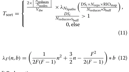
The time estimation of the sort stage is independent on the network, which is shown in Eq. (11). Among them, the calculation of the form is shown in Eq. (12).
Tsort=
The output data of sort is the input of the reduce phase. During this phase, data processing and writing to HDFS are operated simultaneously; thus, we can take the
Table 3The parameters of clusters
Table 4Other related parameters
Type Symbol Value
Cluster Vdw 50.96MB/s
Hadoop&HDFS Nsm 4
Nsr 2
Ncp_threads 30
Vcp_thread 10 MB/s
Vreduce_rep 10 MB/s
NSpths 10
Nreps 3
Sbuff 716
App Mthruput 1.18 MB/s
Rthruput 15.47 MB/s
maximum time of them and the final time of this stage (Eq. (13)).
Treduce=max(Trp,Tro) (13)
Calculating the processing time of one reduce and then multiplied by the number of reduces can get the overall processing time of reduce (Eq. (14)). In this paper, it is assumed that there is only one reduce wave. The circum-stances we considered is transferring all source data to a local data center to build a cluster or setting up clusters simultaneously in respective data centers without trans-ferring source data; therefore, the source data in these two circumstances are different.
The duplication is set as 3 in HDFS, including the orig-inal data set. In this paper, the remote cluster does not exit and all nodes are in the same subnet, so it is not time-consuming to transfer the copy to a remote cluster. One copy will be written to the local hard disk, while the remaining two copies will be stored in other nodes in the local cluster. This process should be limited to the local bandwidth. We choose the maximum time of the local disk writing time and the local clusters writing time as the reduce output writing time (Eq. (15)).
Tro=max
Trp_disk,Trp_local
(15)
The local disk writing time of a copy is equal to the aver-age amount of data written to the local disk in each node divided by the disk write speed (Eq. (16)). The disk write speed is obtained by Bonnie++ [17], a tool for disk I/O performance test.
Trp_disk=
DSi×RIOmap×Nreps
Nnodes∗Vdw
(16)
Because of the assumption that one reduce only produce a single output file and two copies of it will be copied to the other two nodes in local cluster, the copy speed is limited by the bandwidth of the subnet the cluster belongs to. We utilize Eq. (17) to estimate the minimum store speed of each reduce data copy in the local cluster.
Vrp_local=min
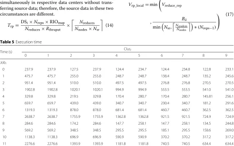
Table 5Execution time
Time (s) Clusi
0 1 2 3 4 5 6 7 8 9
Jobi
0 237.9 237.9 127.5 237.9 124.4 234.7 124.4 234.8 122.8 233.1
1 475.7 475.7 255.0 255.0 248.7 248.7 138.4 248.7 135.2 245.6
2 951.4 951.4 510.0 510.0 497.5 497.5 276.8 276.8 270.5 270.5
3 1902.8 1902.8 1020.1 1020.1 994.9 994.9 553.5 553.5 541.0 541.0
4 329.8 329.8 219.5 329.8 170.4 280.7 170.4 280.7 145.81 256.1
5 659.7 659.7 439.0 439.0 340.7 340.7 230.4 340.7 181.2 291.6
6 1319.3 1319.3 878.0 878.0 681.4 681.4 460.7 460.7 362.5 362.5
7 2638.7 2638.7 1755.9 1755.9 1362.8 1362.8 921.5 921.5 724.9 724.9
8 284.6 284.6 174.2 284.6 147.7 258.1 147.7 258.1 134.5 244.8
9 569.2 569.2 348.5 348.5 295.5 295.5 185.1 295.5 158.6 269.0
10 1138.3 1138.3 696.9 696.9 590.9 590.9 370.2 370.2 317.2 317.2
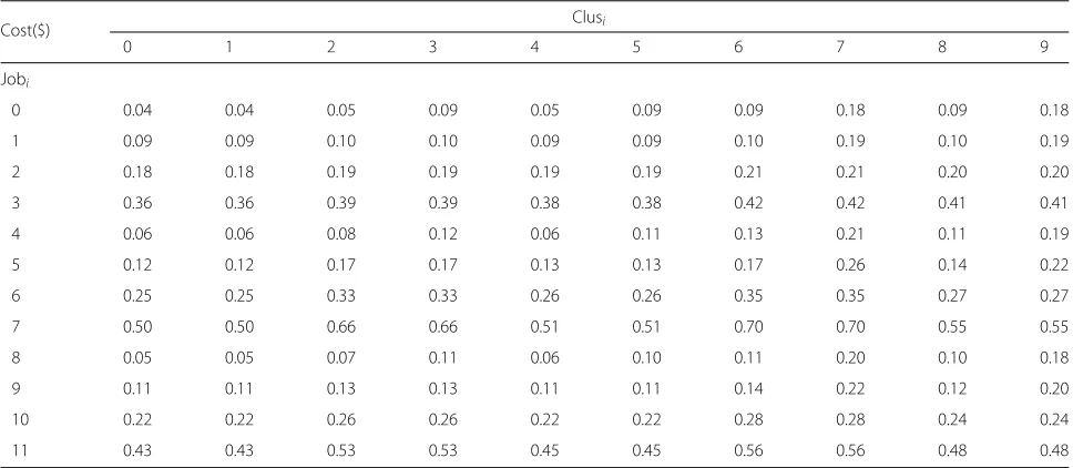
Table 6Execution cost
Cost($) Clusi
0 1 2 3 4 5 6 7 8 9
Jobi
0 0.04 0.04 0.05 0.09 0.05 0.09 0.09 0.18 0.09 0.18
1 0.09 0.09 0.10 0.10 0.09 0.09 0.10 0.19 0.10 0.19
2 0.18 0.18 0.19 0.19 0.19 0.19 0.21 0.21 0.20 0.20
3 0.36 0.36 0.39 0.39 0.38 0.38 0.42 0.42 0.41 0.41
4 0.06 0.06 0.08 0.12 0.06 0.11 0.13 0.21 0.11 0.19
5 0.12 0.12 0.17 0.17 0.13 0.13 0.17 0.26 0.14 0.22
6 0.25 0.25 0.33 0.33 0.26 0.26 0.35 0.35 0.27 0.27
7 0.50 0.50 0.66 0.66 0.51 0.51 0.70 0.70 0.55 0.55
8 0.05 0.05 0.07 0.11 0.06 0.10 0.11 0.20 0.10 0.18
9 0.11 0.11 0.13 0.13 0.11 0.11 0.14 0.22 0.12 0.20
10 0.22 0.22 0.26 0.26 0.22 0.22 0.28 0.28 0.24 0.24
11 0.43 0.43 0.53 0.53 0.45 0.45 0.56 0.56 0.48 0.48
The reduce output data size divided by Eq. (17) is the maximum time of data copies to store in the local cluster (Eq. (18)) .
Trp_local=
DSi×RIOmap×RIOreduce
Nreduce ∗
1 Vrp_local
(18)
The copy phase from the first wave completion of the map results in the overlap between these two phases; thus, the job execution time of one cluster in respective data center is shown as Eq. (19).
Tjob=
Tmap+TNcopymw +Tsort+Treduce, Tmap>Tcopy
Tmap
Nmw +Tcopy+Tsort+Treduce, Tmap<Tcopy
(19)
6 Evaluation
6.1 Setting of the experiment
Suppose we have the following hypothetical scenario: there are 12 data processing jobs and 10 clusters which have specific configuration. This is considered as one of the examples which is discussed in detail in this paper. We utilize Amazon EC2 (Amazon Elastic Compute Cloud) as a test platform. The types of the nodes in the experiment are all m1.large which is one of the node types that AWS supports and their configuration is the same to each other, namely, 64-bit RHEL (short for Red Hat Enterprise Linux) operating system, two core, 7.5-G memory, 2 420-G stor-ages. The cost of each node is $0.34 per hour. The data center is located in US East (Northern Virginia), and the bandwidth we test using Netperf [18] is 282.4 MB/s.
The parameters of jobs and cluster configuration are listed in Tables 2 and 3, respectively. Table 4 shows other related parameters. As illustrated previously, we have 12
jobs and 10 clusters. For each job, it can be allocated to any of the 10 clusters. So, there will be allocation schemes. Our goal for job scheduling is to choose the best alloca-tion scheme from all of the possible schemes using GAs. Before making this decision, we utilize the performance estimation module to predict the execution time and cost which are the decision indicators in GAs. Then, we get a two dimensional time and cost array which is shown in Tables 5 and 6, respectively. From Tables 5 and 6, we can see that different jobs running on the same cluster may not have the same time and cost consumption. Also, same jobs can take different times and costs to finish its execution in different clusters.
In our implementation, we choose to use Java-based GA frameworks. There are some popular implementa-tions, such as JGap [19], ECJ [20], and JMetal [21]. When compared with JMetal’s counter-parts, the design of JMetal has a good separation of concerns in terms of its easiness for applying different GAs after a prob-lem is abstracted. Therefore, JMetal is chosen as the GA framework in our paper. In our evaluations, GA
Table 7Parameters for NSGA-II
Symbol Value
Population size 50
Max evaluations 2000
Crossover operator Single-point crossover
Crossover probability 0.9
Mutation operator Bit-flip mutation
Mutation probability 1/number of variables
Fig. 3Comparison between real measurement and module prediction
Non-dominated Sorting Genetic Algorithm (NSGA-II) is chosen as the concrete algorithm. Algorithm parame-ters setting in our implementation includes the maximum evaluations, the crossover probability, and the mutation operator, as shown in Table 7. As choosing integer chro-mosome, single-point crossover, bit-flip mutation, and Binary tournament2 operators are selected drawing on the experience of [22]. Reference [6] talks about how the operators work to make a change to the chromosome in GAs.
6.2 Results
In order to evaluate the effectiveness of the proposed performance estimation module, we choose US East (Northern Virginia) data center to set up real clusters in Amazon EC2 platform and run some experimental jobs and compare them to the results obtained from per-formance estimation module (Fig. 3). By comparing the results estimated and real results in Fig. 3, we can find that our performance module estimates accurately the data processing time in general. Bandwidth and resource load may lead to delays in real world when compared with predicted time performance, but this part of error can be acceptable. Since the estimation of cost performance depends on the times, so deduce the effectiveness of it from the above conclusion.
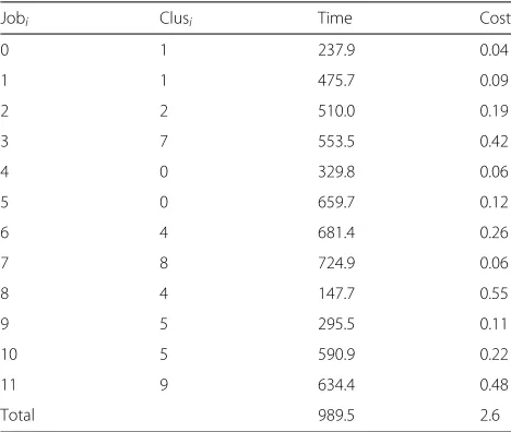
Meanwhile, in order to compare the performance of NSGA-II with other algorithms, we choose simple alloca-tion method for comparison, which is a random allocaalloca-tion policy: all jobs are assigned to a group of clusters ran-domly. We verify and evaluate each job scheduling policy derived by NSGA-II and simple allocation method. The results are shown in Tables 8 and 9, respectively. From these three tables, we can find that the scheme obtained from GA-based approach takes 989.5 time units and $2.6
to finish all of 12 jobs’ execution while the other scheme from a simple method takes 2638.7 time units and $3.10. So, GA-based approach can do the optimized decision and make the data processing have the fastest execution effi-ciency and minimum cost. According to the GA-based scheme, data processing jobs can be finished as fast as possible with the optimized cost, and therefore, users can have better experience and can be more satisfied.
7 Conclusions
Job scheduling is one of the most important issues in big data analytics. In this paper, we propose a genetic algorithm-based approach, which uses a performance estimation module we put forward, for obtaining opti-mized jobs scheduling scheme that have the optiopti-mized
Table 8NSGA-II-based approach
Jobi Clusi Time Cost
0 1 237.9 0.04
1 1 475.7 0.09
2 2 510.0 0.19
3 7 553.5 0.42
4 0 329.8 0.06
5 0 659.7 0.12
6 4 681.4 0.26
7 8 724.9 0.06
8 4 147.7 0.55
9 5 295.5 0.11
10 5 590.9 0.22
11 9 634.4 0.48
Table 9Simple scheduling method
time and cost consumption. The optimized solutions can be used to enable effective scheduling strategies, and then in the actual running, system can make use of the cho-sen scheduling scheme to execute data processing jobs. The whole process is evaluated and the results show that our approach is feasible with acceptable performance and accuracy. Due to the limitations in our performance esti-mation module, currently, the evaluation is simplified and in the future, the approach will be extended to be more complete and precise.
Competing interests
The authors declare that they have no competing interests.
Acknowledgements
This project is supported by the National Natural Science Foundation of China (Grant No. 61402533), the Fundamental Research Funds for the Central Universities (Grant No. 16CX02047A), and the Scientific Research Foundation of China University of Petroleum (Grant No. Y1307021).
Received: 23 December 2015 Accepted: 5 June 2016
References
1. A Hadoop, Apache Software Foundation (2016). http://hadoop.apache.org
2. J Dean, S Ghemawat, MapReduce: simplified data processing on large clusters. Commun. ACM.51(1), 107–113 (2008)
3. M Mitchell, An introduction to genetic algorithms. Journal of Computing Sciences in Colleges.20(1) (2004)
4. A Konak, DW Coit, AE Smith, Multi-objective optimization using genetic algorithms: a tutorial. Reliab. Eng. Syst. Saf.91(9), 992–1007 (2006) 5. K Deb, An introduction to genetic algorithms. Sadhana.24(4–5), 293–315
(1999)
6. SM Thede, An introduction to genetic algorithms. J. Comput. Sci. Coll. 20(1), 115–123 (2004)
7. E Amazon, Amazon elastic compute cloud (amazon ec2). Amazon Elastic Compute Cloud (Amazon EC2) (2015). https://aws.amazon.com/ec2/ 8. J Berli ´nska, M Drozdowski, Scheduling divisible mapreduce
computations. J. Parallel Distrib. Comput.71(3), 450–459 (2011) 9. T Nykiel, M Potamias, C Mishra, G Kollios, N Koudas, MRShare: sharing
across multiple queries in MapReduce. Proc. VLDB Endowment.3(1–2), 494–505 (2010)
10. M Zaharia, A Konwinski, A Joseph, R Katz, I Stoica, inProceedings of OSDI 201. Improving MapReduce performance in heterogeneous
environments, (2008), pp. 29–42
11. L Xu, inParallel and Distributed Processing Symposium Workshops & PhD Forum (IPDPSW), 2012 IEEE 26th International. MapReduce framework optimization via performance modeling (Shanghai, China, 2012), pp. 2506–2509
12. J Han, M Ishii, H Makino, inComputer Science and Information Technology (CSIT), 2013 5th International Conference on. A Hadoop performance model for multi-rack clusters, (Amman, Jordan, 2013), pp. 265–274
13. S Krishan Veer, R Zahid, inComputer Engineering and Applications (ICACEA), 2015 International Conference on Advances in. A GA based job scheduling strategy for computational grid, (Ghaziabad, India, 2015), pp. 29–34 14. A Syed Hasan, R Kamran, in2015 International Conference on Open Source
Systems & Technologies (ICOSST). Cloud task scheduling using nature inspired meta-heuristic algorithm, vol 2 (IEEE, 2015), pp. 158–164 15. K Shvachko, H Kuang, S Radia, R Chansler, in2010 IEEE 26th Symposium on
Mass Storage Systems and Technologies (MSST). The hadoop distributed file system, (Nevada State, Molossia, 2010), pp. 1–10
16. T White,Hadoop: The definitive guide. (O’Reilly Media, April 2015) 17. Bonnie, Bonnie++ (2012). http://sourceforge.net/projects/bonnie/.
Accessed 19 July 2015
18. Netperf, Netperf (2012). http://www.netperf.org/netperf/. Accessed 19 July 2015
19. DY Chen, TR Chuang, SC Tsai, JGAP: a Java-based graph algorithms platform. Softw. Pract. Experience.31(7), 615–635 (2001) 20. site, site (2015). https://cs.gmu.edu/~eclab/projects/ecj/.
Accessed 19 July 2015
21. JJ Durillo, AJ Nebro, jMetal: a Java framework for multi-objective optimization. Adv. Eng. Softw.42(10), 760–771 (2011)
22. W Zhang, KM Hansen, inEngineering of Complex Computer Systems, 2009 14th IEEE International Conference on, IEEE. An evaluation of the NSGA-II and MOCell genetic algorithms for self-management planning in a pervasive service middleware, (2009), pp. 192–201
Submit your manuscript to a
journal and benefi t from:
7Convenient online submission 7Rigorous peer review
7Immediate publication on acceptance 7Open access: articles freely available online 7High visibility within the fi eld
7Retaining the copyright to your article