Research on the 3D imaging algorithm of spin target based on the Hough transform

R E S E A R C H

Open Access

Research on the 3D imaging algorithm of spin

target based on the Hough transform

Jin Li

and Yiming Pi

Abstract

As one of the most typical characteristics in space target motion, spin phenomenon has good 3D imaging application potential. Conventional target imaging algorithm fails to make full use of the rotating features of the target to obtain the characteristics of target space, and the speedy spin of targets will cause the dramatic changes in the positions of scattering center within short observation session, which may lead to the failure of imaging algorithm. Aiming at such a special phenomenon of the space target, the time frequency distribution curve of echoes in each scattering center could be mapped onto the parameter space to obtain the position of each scattering center by taking advantage of Hough transformation, thus the 3D features of spin target could be obtained. In this article, the 3D imaging algorithm was studied on the basis of Hough transformation, and its effectiveness was tested with simulation. Meanwhile, the translational motion and shielding effect of space target were discussed, and favorable imaging results were achieved.

Keywords:3D imaging, Spin target, Hough transform, ISAR

1. Introduction

Study on the 3D inverse synthetic aperture radar (ISAR) imaging techniques has been attracting more and more attention [1-6]. Compared to 2D ISAR imaging tech-niques, more detailed information about the target can be provided by 3D ISAR imaging. The current 3D ISAR imaging algorithm mainly consists of two types. The first type takes advantage of various reception channels and receives the echo signals of the target on the basis of phase interference, and it can conduct 2D image for the signals received by each antenna with conventional im-aging algorithm [7-9]. As a result, the three-dimensional spatial information of each scattering point can be extracted from the differences of 2D imaging interfer-ence phase. In the second type, the target 3D imaging is constructed with the 2D image sequence obtained from different observation angle through a receiving antenna [10]. In both algorithms, a spatial freedom degree is added to obtain three-dimensional resolution.

The traditional ISAR imaging algorithm is based on slow turntable model. High-speed rotating targets, such as airplane propeller, spin precession-guided missile warhead,

space debris, etc., often fail to meet the requirements of slow turntable model. However, for spin target, its rotating angular velocity can be estimated, which in actually pro-vides a degree of freedom for 3D ISAR imaging [11,12]. As in [13,14], on the condition of the turntable model with high-speed rotating target and its spin angular velocity is known, the methods general radon transform and extended Hough transform were used to three-dimensional space information extraction for rotating targets. The basic idea of these algorithms is taking advan-tage of sine envelope of spin target to estimate the

scatter-ing points’three-dimensional location by using curvilinear

integral under range-compress domain. The operand of these algorithms is always huge because the energy accu-mulation along curve is four-dimensional curve detection process. In this article, sine envelope of spin target was used to estimate the 3D position of scattering point in the form of curvilinear integral within distance compressed domain, thus the extraction of 3D spatial information of the spin target could be realized.

2. Target and echo signal model

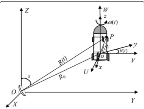
As shown in Figure 1, radar was seated in the originOof

radar coordinateO-XYZ, the projection of radar sight axis

on OXY plane was in the same direction and coincided

* Correspondence:[email protected]

College of Electronic Engineering, University of Electronic Science and Technology of China, Chengdu 611731, China

withY-axis, and the included angle of radar sight axis and

Z-axis was α. Reference frame o-UVW paralleled to

co-ordinate systemO-XYZ, and both corresponding

coordin-ate axes pointed to the same direction. The originowas

seated in the target rotation axis, axisWwas the direction

of angular velocity vector of target rotation, axesU, V, and

Wformed right-handed rectangular coordinate system. In

O-XYZ coordinate, the coordinate of pointowas (X0,Y0,

Z0), and obviously X0= 0. The distance between two

co-ordinate originsOandowasR0, and then

R0¼

The target coordinate system o-xyz and reference

co-ordinate system o-UVW shared the same origin, both

the axeszand Wpointed to the same direction, and the

target coordinate system o-xyzrotated with the targets.

Initially, t0= 0, the target coordinate system o-xyz and

reference coordinate system o-UVW coincided, and at

momentt, the included angle of the two coordinate

sys-tems wasθ(t), namely

θð Þ ¼t Z t

0 ω τ

ð Þdτ ð3Þ

The coordinate of any scattering pointPin coordinate

systemo-xyz was (xP,yP, zP), while it was (uP, vP, wP) in

coordinate system, obviously

zP¼wP ð4Þ

The distance between P and the origin o was rP, the

coordinate ofPin coordinate systemO-XYZwas (XP, YP,

When the geometric dimensioning of target was far smaller than the distance between the target and radar, namely it metuP<<R0,vP<<R0, whenwP<<R0, Equation (5) could be approximated as the following equation:

RPð Þt ≈R0þ

Project the 3D figure in Figure 1 onto oUVplane, as

shown in Figure 2, then there was the following coordin-ate transformation relation:

uP¼xPcosθð Þ t yPsinθð Þt

vP¼xPsinθð Þ þt yPcosθð Þt

ð7Þ

Substitute Equations (2), (4), and (7) into Equation (6), it could be obtained

RPð Þt ≈R0þ Figure 1Geometric model for the spatial position relation of

spin target.

Assume the target took uniform rotating motion, namely

ω(t) =ω, was a constant, then

θð Þ ¼t ω⋅t ð9Þ

Substitute it into Equation (8)

RPð Þ ¼t R0þxPsinαsinωtþyPsinαcosωt

þzPcosα ð10Þ

To make it simple, assume

xPsinα¼x

radar linear frequency modulation (LFM) signal

sðt~Þ ¼rect t~

In which,Tis the pulse width,f0is carrier frequency,γ

is time-frequency rate, rectð_Tt~Þ is rectangular window

function, defined as

rect t~

The instantaneous frequency of LFM signal was

f ¼f0þγt~;t~j≤T=2

In which,B=γTwas the signal bandwidth.

Assume the reflection coefficient of scattering point P

within observation time was constantσP, then the radar

echo of this point could be represented as

sPðf;tÞ ¼σPW fð ;tÞexp

observation time, Tobs is the total time-bandwidth of

the observation, and c is the speed of light. Substitute

Equation (12) into Equation (16), and compensate

for the constant phase term brought by R0, it could be

obtained

In radar imaging, the scatterer model was often adopted to describe targets, and the target echo could be seen as the sum of each scattering point echo. For a spin

target formed from K scattering points, its

correspond-ing coordinate and reflection coefficient were (xk,yk, zk)

andσk(k= 1, 2,. . .,K), then the target echo could be

rep-Conduct inverse Fourier transform for f in Equation

(18), the data after range compression could be obtained, namely the range residence time domain data, as shown in the following equation:

S rð ;tÞ ¼IFTfs fð ;tÞg

3.3. D imaging algorithm

It could be seen from Equation (19) that, owning to the target spin, the position of range data peak of each scat-tering point corresponding to the range residence time domain would change according to the range of this scattering point within observation time. Such periodical variation of the peak could be approximated with a sine curve. That is to say, the position of each scattering point in range direction could be approximated as a sine curve, satisfying the following equation:

r¼xk

On the premise of given sine curve cycle (namely ω

three spatial coordinate parametersxk',yk', andzk'. There-fore, the 3D position information of the scattering point could be obtained by extracting the information about sine curve.

However, it could be seen from the above analysis that,

owning to the influence of the included angleαbetween

the radar sight and target axis, the actually extracted position information of scattering point was not authen-tic position information, but the compression of real position, namely, the position coordinate extracted along

the axis direction (namely along axisz) was about cosα

times of the real position coordinate, while the position coordinate which was vertical to spin axis (namely along

axes x andy) was about sinα times of the real position

coordinate. Therefore, the smaller α was, the closer the

coordinate along axis z would be. The better the

reso-lution along axis z was, the worse the resolution along

axesxandywould be, and vice versa.

For a target formed from one or several scattering points, the target echo was the sum of each scattering point. Therefore, sine curves might tangle with each other. In addition, with imaging treatment period, each scattering point may not always be shone by the radar beam owning to the shield, namely the scattering point may not have echo. Therefore, there might be discon-tinuities in sine curve. As a result, it was a little difficult to directly detect the sine curve within range residence time domain, also the image domain. Each sine curve in the image domain corresponded to a peak in the param-eter domain, and the paramparam-eter corresponding to the peak was the 3D position coordinate of the scattering point. Consequently, with the help of Hough transform-ation, the detection for the global curve in the image do-main could be converted to detection of peaks in easily realized parameter domain.

The Hough transformation of the image was the cu-mulates along the transformation curve, defined as fol-lows:

In the above equation,d(Φ) was the Hough

transform-ation result of image D(m,n), Φ was the

multi-dimensional vectors formed by related curve parameters,

n =f(m; Φ) was the curve to be detected. Here,m was

the corresponding residence timet, the curve parameter

vector Φ consisted of three positional parameters,

namelyx0_k,y0_k, andz_k0,f(m;Φ) corresponded to the curve

r=xk' sinωt+yk' cosωt+zk' in the image for range

resi-dence time domain.

By equation (19), the image for range residence time domain could be obtained:

G rð ;tÞ ¼jS rð ;tÞj ð22Þ

Then its Hough transformation was shown in the fol-lowing equation

After Hough transformation, the corresponding curve of each scattering point in range residence time domain would produce a peak in the parameter domain. The es-timation for the spatial position of scattering point could easily be realized through detecting the peaks in param-eter domain.

Owning to the limited signal bandwidth, there might be certain width in the main lobe of the echo of scatter-ing point after range compression and many side lobes, which would add to the difficulty in actual detection and bring unfavorable influence for imaging, such as the loss of real scattering point, production of fake scattering point, etc. Therefore, the information of each scattering point could be obtained by combining the target param-eter estimation method and CLEAN technology. That is

to say, after the 3D position coordinate x0_k;y0_k;z0_k was

obtained, the point spread functionX(r,t) of the

scatter-ing point with unit-strength scatterscatter-ing coefficient at this position was constructed according to Equation (19) as follows:

According to certain standard and taking advantage of

S(r,t) and X(r,t), the scattering coefficient of scattering

point in this position could be estimated.

For example, the estimation of scattering coefficient could select the following minimum norm criterion:

In order to solve Equation (25), adopt derivative about

σfromI(σ), and suppose it as 0, namely

∂Ið Þσ

∂σ ¼ 2

X

r;t

S rð ;tÞ σX rð ;tÞ

½ Xðr;tÞ ¼0 ð26Þ

In which, X*(r, t) was the conjugation ofX(r,t). Then

the estimation value ^σ of scattering coefficient could be

obtained

^

σ ¼

X

r;tS rð;tÞX

r;t

ð Þ

X

r;tjX rð ;tÞj

2 ð27Þ

After the information about 3D position and scattering co-efficient of this scattering point was obtained, the informa-tion about this scattering point in the echo data was

eliminated, namely supposeS rð ;tÞ ¼S rð;tÞ ^σX rð ;tÞ, and

the above procedures of parameter estimation were

re-peated with new data S(r, t), till σ^ was smaller than the

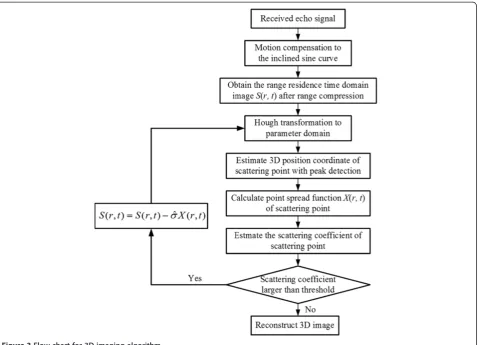
pre-set threshold. At this moment, the information of all scattering points was extracted from echo data, and 3D image of the target could be reconstructed with the information.

In practice, sinc function was characterized with certain main lobe width, and together with the interference of echo side lobe of other scattering points and the influence of parameter discrete step in parameter domain, there might be differences between the parameters extracted in the Figure 3Flow chart for 3D imaging algorithm.

Table 1 Coordinate and scattering coefficient of each scattering point

Number Coordinate of 3D position Scattering_{coefficientσ}

x(m) _y(m) _z(m)

1 0:3pffiffiffi2 0 0:6pffiffiffi2 1.3 2 0 0:3pffiffiffi2 0:6pffiffiffi2 1.0 3 0:3pffiffiffi2 0 0:6pffiffiffi2 1.0 4 0 0:3p2ffiffiffi 0:6pffiffiffi2 1.0 5 0:2pffiffiffi2 0:2pffiffiffi2 0:3pffiffiffi2 1.3 6 0:2pffiffiffi2 0:2pffiffiffi2 0:3pffiffiffi2 1.0 7 0_:2pffiffiffi2 0_:2pffiffiffi2 0_:3pffiffiffi2 1.0 8 0:2pffiffiffi2 0:2pffiffiffi2 0:3pffiffiffi2 1.0

parameter domain after Hough transformation and actual coordinate. At this moment, the coordinate value with errors were adopted for constructing point spread function, then there might be relatively large errors in the scattering coeffi-cient obtained, which would influence the performance of CLEAN algorithm and lead to the decrease in the perform-ance of 3D imaging algorithm. In order to improve the accuracy of the estimation for the position of scattering point and scattering coefficient, the following thought could be adopted: the estimated value of the information of scattering point was obtained through Hough transformation, the esti-mated value was adopted as the initial value, and then param-eters satisfying Equation (28) were searched with small step around the scattering point, which would be regarded as the final estimated value of the scatterer parameter.

^x0_k;^y_k0;^z_k0;^σ

The specific flow chart for 3D imaging algorithm was shown in Figure 3.

4. Simulation experiment

The signal bandwidth was 4 GHz, while the time

band-width was 4 μs. The pulse repetition frequency was 0.6

kHz. Assume that the included angle of radar sight and

target spin axis wasπ/4, the distance between the target

center and radar was about 14.14 km, the angular vel-ocity of the target spin was 5 Hz. In this equation, the translation component of the target should be compen-sated well to make sure that the included angle of the radar sight and spin axis should remain unchanged when the target spun in high speed. Radar far-field target formed by nine scattering point shall be established as shown in Table 1, in addition, this target also had

vel-ocity componentve= 1/salongzdirection.

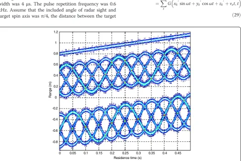
The image of range residence time domain was shown in Figure 4, and obviously owing to the velocity

compo-nent in z direction, the position of scattering points

changed continuously. As a result, the center of sine

curve also changed continuously, namely ‘inclined’ sine

curve was formed.

In order to make up for the translation component, the

‘inclined’sine curve could be corrected. And the curve

ex-pression could be adjusted during Hough transformation,

namely to substitutez0_k withz0_kþvetin Equation (23), the

corresponding Hough transformation could be changed to the following form:

g x0_k;y0_k;z_k0;ve

Residence time (s)

Range (m)

0.8

0.6

0.4

0.2

0

-0.2

-0.4

-0.6

-0.8

Range (m)

0 0.05 0.1 0.15 0.2 0.25 0.3 0.35 0.4 0.45

Residence time (s)

Figure 6The image of range residence time domain after compensating the translation component. 7

6

5

4

3

2

1

0 0.05 0.1 0.15 0.2 0.25 0.3 0.35 0.4 0.45 0.5

Residence time (s)

Correlation coefficient

One or several scattering points could be used to

ob-tain the estimation value ^ve of translational velocity,

which would compensate for the translation component caused by this speed. However, the original 3D

param-eter domainx0_k;y0_k;z0_kwould be added to 4D parameter

domain x0_k;y0_k;z0_k;ve

. When estimating the parameter, 4D search was needed. Therefore, this method would greatly increase the calculated amount.

In order to decrease the calculated amount, slide correlation-based method could be adopted. According

90

0.8 0.6 0.4 0.2

0

x (m)

magnitude

80

70

60

50

40

30

20

y (m) _{-0.5 -0.4} -0.6 -0.8

0.5

0

-0.2

Figure 8The results of parameter domain after Hough at point (z=−0.6 m) in plane z. 5.5

5

4

3

2

1

0 0.05 0.1 0.15 0.2 0.25 0.3 0.35 0.4 0.45 0.5

Residence time (s)

Correlation coefficient

4.5

3.5

2.5

1.5

to the position of maximum correlation coefficient, the translation component could be compensated. In Figure 5, the maximum correlation coefficient of the

first echo (namely echo at t = 0) and other echoes.

Owning to the good symmetry among each scattering point, the peak would occur at the quarter of each

rotation cycle. The range residence time domain after compensation was shown in Figure 6, and obviously the translation component was compensated well. At this moment, subsequent algorithm such as Hough trans-formation, etc., could be conducted, and 3D imaging could be realized.

1

0.5

0

-0.5

-1

0 0.05 0.1 0.15 0.2 0.25 0.3

Residence time (s)

Range (m)

Figure 10The range residence time domain image of multi-scattering points after taking shield into consideration. -0.4

-0.2 0

0.2

0.4

-0.4 -0.2 0 0.2 0.4 -0.6 -0.4 -0.2 0 0.2 0.4 0.6 0.8

0.9957

1.3126

x(m) 0.9985 1.3364 0.9997

1.0272

1.0133

0.9982 1.0051

y(m)

z(

m

)

When there was a lack of good symmetry in each tar-get scattering point, if only seven scattering points were

selected, such as the①②③⑤⑥⑦⑨ in Table 1, the

ma-ximum correlation coefficient of echo att= 0 and other

moments were shown in Figure 7. Obviously, the ma-ximum peak would occur only when the rotation cycle was in integral multiple. For the unknown rotation cycle,

this method could also be used to estimate the spin cycle of the target.

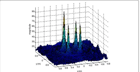
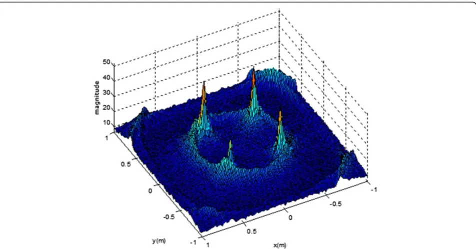
As shown in Figure 6, the image of range residence time domain was transferred to parameter domain after

Hough transformation, the result was cut out at z =

−0.6, as shown in Figure 8. There were four scattering

points in this plane, therefore, it would form four

-0.4

-0.2 0

0.2

0.4

-0.4 -0.2 0 0.2 0.4 -0.6 -0.4 -0.2 0 0.2 0.4 0.6 0.8

0.9958

1.3121

x(m) 1.0133 1.3361 0.9997

1.0269

0.9986

0.9982 1.0054

y(m)

z(

m

)

Figure 12Results of 3D imaging after taking shield into consideration.

distinct peaks in the parameter domain, and the corre-sponding parameter information was the spatial position information of the scattering point. Besides, owning to the influences of such factors as the side lobes of each scattering point, there were small fluctuations in the par-ameter domain.

The final 3D imaging result was shown in Figure 9.

Since the radar sight angleα=π/4, the coordinate value

in the direction of axesx,y, andzwas aboutpffiffiffi2=2 times

of the real value. In the figure, the marked figures were the estimated value of the scattering coefficient of the scattering point at corresponding position obtained from this algorithm. It could be seen from the figure that 3D imaging could be realized from this algorithm.

Since it was unavoidable that the scattering center of the spin target was seated in the back of radar sight, it was impossible for each scattering center to be shone by the radar beam. Therefore, the shielding condition in the scattering center should be considered. The range resi-dence time domain image after taking shield into consid-eration and transformational results of parameter domain were shown in Figures 10 and 11, respectively, in which the parameter of each scattering point was shown in Table 1. Within image observation period,

scattering point⑨on the spin axis could always be seen,

while the rest eight ones could be seen within half cycle close to radar. It could be seen from Figure 10 that owning to the influence of shield, the sine curve in the image domain was discontinuous, and at this moment, it was difficult to directly detect the curve. There was obvi-ous peak in the parameter domain shown in Figure 11, which was easier to detect the parameter.

The results of 3D imaging after taking shield into con-sideration were shown in Figure 12, and obviously, it could also obtained good imaging results.

5. Conclusion

In this article, 3D imaging algorithm of spin target based on Hough transformation was proposed. By taking advan-tage of the sine envelope of spin target, the 3D position of scattering point was estimated in the form of curve integral within range compression domain, thus the extraction of 3D spatial information of the spin target could be realized, and this algorithm was tested to be valid through simula-tion experiment. In addisimula-tion, the translasimula-tional mosimula-tion and shielding condition existed in the real target were also taken into consideration in the simulation experiment, and corresponding measures were adopted for translational mo-tion compensamo-tion. Under the circumstance of incomplete target sine curve, the target parameter was extracted to realize the 3D imaging of spin target.

Competing interests

The authors declare that they have no competing interests.

Acknowledgement

This study was supported by the National Natural Science Foundation of China (61271287) and the Fundamental Research Funds for the Central Universities (ZYGX2011J020).

Received: 5 December 2012 Accepted: 28 February 2013 Published: 28 March 2013

References

1. VC Chen, F Li, SS Ho et al., Analysis of micro-Doppler signatures. IEE Proc. Radar Sonar Navigat.150(4), 271–276 (2003)

2. Q Zhang, TS Yeo, G Du, SH Zhang, Estimation of three dimensional motion parameters in interferometric ISAR imaging. IEEE Trans. Geosci. Remote Sens.42(2), 292–300 (2004)

3. J Tsao, BD Steinberg, Reduction of sidelobe and speckle artifacts in microwave imaging: the CLEAN technique. IEEE Trans. Antennas Propagat. 36(4), 543–556 (1988)

4. T Sparr, B Krane, Micro-Doppler analysis of vibrating targets in SAR. Proc. Inst. Electr. Eng.-Radar Sonar Navigat.150(4), 277–283 (2003)

5. J Li, YM Pi, Micro-Doppler signature feature analysis in terahertz band. J. Infrared Millim. Terahertz Waves31(3), 319–328 (2010)

6. J Li, H Ling, Application of adaptive chirplet representation for ISAR feature extraction from targets with rotating parts. Proc. Inst. Electr. Eng.-Radar Sonar Navigat.150(4), 284–291 (2003)

7. GY Wang, XG Xia, VC Chen, Three-dimensional ISAR imaging of maneuvering targets using three receivers. IEEE Trans. Image Process. 10(3), 436–448 (2001)

8. XJ Xu, RM Narayanan, Three-dimensional Interferometric ISAR imaging for target scattering diagnosis and modeling. IEEE Trans. Image Process. 10(7), 1094–1102 (2001)

9. JT Mayhan, ML Burrows, KM Cuomo, JE Piou, High resolution 3D“snapshot” ISAR imaging and feature extraction. IEEE Trans. Aerosp. Electron. Syst. 37(2), 630–642 (2001)

10. JL Walker, Range-Doppler imaging of rotating objects. IEEE Trans. Aerosp. Electron. Syst.AES-16(1), 23–52 (1980)

11. KV Hansen, PA Toft, Fast curve estimation using preconditioned generalized radon transform. IEEE Trans. Image Process.5(12), 1651–1661 (1996) 12. PA Toft, Using the generalized radon transform for detection of curves in

noisy images, IEEE International Conference on Acoustics, Speech and Signal Processing, Atlanta, USA, vol. IV, 1996, pp. 2219–2222

13. Q Wang, MD Xing, High-resolution three-dimensional radar imaging for rapidly spinning targets. IEEE Trans. Geosci. Remote Sens.

46(1), 22–30 (2008)

14. Q Zhang, TS Yeo, Imaging of a moving target with rotating parts based on the Hough transform. IEEE Trans. Geosci. Remote Sens.

46(1), 291–299 (2008)

doi:10.1186/1687-1499-2013-90

Cite this article as:Li and Pi:Research on the 3D imaging algorithm of

spin target based on the Hough transform.EURASIP Journal on Wireless Communications and Networking20132013:90.

Submit your manuscript to a

journal and benefi t from:

7 Convenient online submission 7 Rigorous peer review

7 Immediate publication on acceptance 7 Open access: articles freely available online 7 High visibility within the fi eld

7 Retaining the copyright to your article