Three-dimensional viscoelastic interseismic deformation model
for the Cascadia subduction zone
Kelin Wang, Jiangheng He, Herb Dragert, and Thomas S. James
Pacific Geoscience Centre, Geological Survey of Canada, 9860 W. Saanich Rd., Sidney, B.C., Canada V8L 4B2
(Received May 18, 2000; Revised September 19, 2000; Accepted September 26, 2000)
Contemporary deformation of the Cascadia forearc consists of an elastic interseismic strain build-up as part of the subduction earthquake deformation “cycle” and a secular deformation primarily in the form of arc-parallel translation and clockwise rotation of forearc blocks. A three-dimensional (3-D) elastic dislocation model, constrained by vertical deformation data, was developed previously to study the interseismic deformation. In this study, we develop a 3-D viscoelastic finite element model for the Cascadia subduction zone to study the temporal and spatial variations of interseismic deformation, and we compare the model results primarily with horizontal geodetic deformation observations. The model has an elastic lithosphere/slab and a viscoelastic mantle which has a viscosity of 1019Pa s
as constrained by recent postglacial rebound analyses. For comparison, we adopt a seismogenic zone geometry that was used in the previous elastic dislocation model, and we test the effects of different estimates of relative plate motion on the model predictions. Interseismic deformation is simulated by assigning a backslip rate to the locked zone of the subduction fault, preceded by an earthquake rupture of the same zone. Based on preliminary model results, we draw the following conclusions: (1) The deformation rate decreases through the interseismic period. A seaward motion is predicted for inland sites early in the interseismic period, an effect of postseismic creep of the mantle. (2) Model strain rates 300 years after the earthquake are consistent with the observed values, regardless of the plate motion models used. The horizontal velocities in northern Cascadia decrease landward at a slower rate than predicted by the elastic dislocation model, providing a better fit to observations. (3) Oblique subduction causes strain partitioning. As a result, the direction of local maximum contraction is much less oblique than plate convergence. The northerly direction of the GPS velocities in southern Cascadia represent a northward translation of the forearc. The secular deformation of the forearc may be partially accommodated through earthquake deformation cycles, but it may be better modeled as a process independent of the earthquake cycle.
1.
Introduction
The Cascadia forearc deforms in great subduction earth-quake sequences. The great earthearth-quake sequence is usually called the earthquake cycle, but the word cycle here does not imply a uniform recurrence time. The locking and un-locking of the subduction fault perturbs crustal stresses and causes primarily elastic deformation. The magnitude of the stress perturbation is very small when compared with the background tectonic stresses, but the associated deformation has a fast rate (Wanget al., 1995), a situation similar to the Nankai subduction zone in Southwest Japan (Wang, 2000). Consequently, contemporary geodetic deformation at Cas-cadia is dominated by elastic strain accumulation due to the locking of the subduction fault. For the study of long-term permanent deformation and crustal earthquakes, the inter-seismic strain becomes major contaminating noise. Only when such “noise” is properly modeled and understood, can geodetic data be used to constrain the long-term deforma-tion (Wellset al., 1998). In contrast, for the assessment of hazards caused by great earthquakes, the interseismic elastic strain provides crucial information on the locked zone.
The interseismic deformation of the Cascadia forearc has
Copy right cThe Society of Geomagnetism and Earth, Planetary and Space Sciences (SGEPSS); The Seismological Society of Japan; The Volcanological Society of Japan; The Geodetic Society of Japan; The Japanese Society for Planetary Sciences.
been modeled using two-dimensional (2-D) and three-dimensional (3-D) elastic dislocation models (Dragertet al., 1994; Hyndman and Wang, 1995; Fl¨ucket al., 1997) and a 2-D viscoelastic finite element model (Wanget al., 1994). In this paper, we report preliminary results of a 3-D viscoelas-tic finite element model. A 3-D model takes into account along-strike variations of fault geometry and plate conver-gence parameters. A viscoelastic model incorporates our present knowledge of rock rheology, in particular the time dependent viscous deformation of the mantle.
2.
Summary of Geodetic Observations
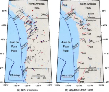
Figure 1(a) is a compilation of published velocities from Global Positioning System (GPS) measurements. Most of the velocity vectors were obtained through campaign style measurements, in which each site was occupied a few times over a period of one to several years (Goldfinger, personal communication, 1999; Khazaradzeet al., 1999; Savageet al., 1991, 2000; Henton, 2000). The earliest regional continuous GPS site was established at Penticton, British Columbia, in 1991 (Dragertet al., 1995). The vectors for the Canadian continuous stations in Fig. 1(a) were reported by Hentonet al. (1999), and those for a few of the U.S. continuous stations by Khazaradzeet al. (1999) and Miller et al. (2001). All velocities are displayed relative to station DRAO (Penticton). Those that were originally reported relative to stable North
Fig. 1. (a) Summary of published GPS velocities in the Cascadia subduction zone. All velocities are relative to reference station DRAO in British Columbia. Grey arrows are results of campaign style GPS measurements. Color arrows are results determined at continuous monitoring stations (shown as red squares) by different groups: red-Pacific Geoscience Centre, green-University of Washington (Khazaradzeet al., 1999), blue-Central Washington University (Milleret al., 2001). Open arrows indicate plate convergence vectors predicted by the new Juan de Fuca-North America Euler pole of DeMets and Dixon (1999) and the NUVEL-1A Juan de Fuca-Pacific pole (Wilson, 1993; DeMetset al., 1994) (see Table 1 for pole position and rotation rate). (b) A summary of geodetic strain rate measurements compiled from triangulation, laser ranging, and GPS observations. A red solid bar indicates contraction, and a blue solid bar indicates extension. A hollow red bar indicates maximum contraction rate where only shear strain rates were determined, assuming uniaxial contraction. Each value represents an average over the area of the strain network used. All data in the U.S. have been compiled or obtained by Murray and Lisowski (2000).
America have been converted using the DRAO velocities relative to North America reported in the same works. One exception is the results in southern Oregon (Savageet al., 2000) for which the necessity of such conversion is being evaluated (Savage, personal communication, 2000).
The uncertainties in the GPS velocities in Fig. 1(a) vary tremendously from site to site. Factors affecting the quality of campaign data include the total time span of the observa-tions, the number of occupations of each station, the length of recording in each occupation, the change of receivers and anntenas from one survey to the next, the experience of the
field workers, and details of data reduction. Reported results for some of the sites, and the associated geophysical inter-pretation, have seen substantial changes as the total time span of the observation becomes longer. Even for the much more reliable continuous data, there exists a discrepancy be-tween velocities derived from the same stations using differ-ent processing procedures. The vectors derived by the Cen-tral Washington University (Miller, personal communication, 2000) for the Canadian stations are generally oriented about 10◦more northerly. Different groups at times used different definitions of stable North America which result in slightly different DRAO velocities. Formal statistical error ellipses
may not be sufficient to represent errors from all sources. Despite the large uncertainties, two features appear robust in the GPS velocities: (1) seaward sites generally have larger velocities in the plate convergence direction than landward sites, and (2) the direction of the velocities becomes increas-ingly northerly as one proceeds from north to south. The
Con-sequently, to study internal deformation, it is necessary to consider the strain ratefield, which is free from rigid-body translation and rotation.
Figure 1(b) is a summary of geodetic strain rate observa-tions in the Cascadia forearc. Strain rates for Canadian net-works JST and GOL were reported by Dragert and Lisowski (1990), QCS and PAL by Dragert (1991), and CVI and SVI by Henton (2000). In the United States, the strain rates were reported by various workers as summarized by Murray and Lisowski (2000). Early triangulation surveys are character-ized by precise measurement of angles but poor control of baseline lengths. Consequently, strain estimates based on repeated surveys where one or both surveys use triangula-tion are limited to shear strain only. Maximum contractriangula-tion rates from such a combination of surveys are derived under the assumption of uniaxial contraction. These are shown in Fig. 1(b) as open bars. Later surveys were conducted us-ing laser rangus-ing or GPS. Repeated measurements usus-ing this technology yield estimates of the full strain rate tensor and the corresponding principal strain rates are shown as solid bars in Fig. 1(b). Almost all strain rates shown in Fig. 1(b) are based on campaign measurements. The shear strain estimates gen-erally provide averages over time periods of several decades, whereas estimates of strain tensors tend to be averages over several (and more recent) years.
The biggest difference between the patterns of geodetic strain rates and GPS velocities is that the direction of maxi-mum contraction near the coast (Fig. 1(b)) changes much less along strike than the change in direction of the GPS velocities (Fig. 1(a)). In regions such as at CAB (Cape Blanco), the northern components of the GPS velocities and their land-ward decrease represent primarily rigid-body motion (Savage et al., 2000). By deriving strain rates, such rigid-body mo-tion, together with any uncertainties with regard to reference frames, have been“filtered out”. This is to say, as the area covered by the CAB GPS network moves northward and ro-tates clockwise, it is being shortened in a nearly E-W direc-tion. The lack of evidence for permanent shortening in this direction suggests that the nearly margin-normal contraction must be elastic. This contraction is the accumulation of strain energy for future great subduction earthquakes.
Except at the northern and southern termini of the subduc-tion zone and near the volcanic arc where fast deformasubduc-tion may take place in relation to triple junction instability or mag-matic processes, the geodetic strain rates in Fig. 1(b) largely reflect interseismic elastic strain accumulation. Interseismic deformation models are better constrained by these strain data than by the GPS vectors in Fig. 1(a) because the GPS vectors include rigid-body motion. Disagreements between GPS velocities and interseismic dislocation model predic-tions have been previously attributed to secular forearc de-formation not accounted for by the model (Khazaradzeet al., 1999). Our 3-D viscoelastic model in the present work is designed to model interseismic deformation only. When the interseismic deformation is properly modeled, it can be
“removed” from the GPS vectors in an approximate fash-ion. The remaining part of the GPS velocities can be used to constrain other geological processes.
3.
Elastic Dislocation Model versus Viscoelastic
Model
The rate of interseismic crustal deformation changes with time, generally faster just after a great earthquake and slower afterwards. The best example is the variation of vertical crustal displacement rates before and after the 1944/46 great earthquakes along the Nankai subduction zone; repeat lev-eling across the margin since the late nineteenth century has clearly demonstrated such time dependence (Thatcher, 1984; Miyashita, 1987).
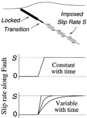
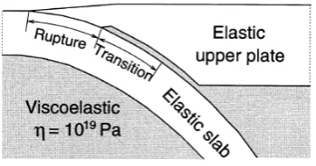
The elastic dislocation model is well known to describe static (i.e., excluding wave propagation) coseismic deforma-tion of the crust accurately. It is also customary to use the dislocation model, in a reverse sense, to describe interseis-mic deformation. For a subduction fault (Savage, 1983), a shallow portion is assumed to be locked, and from a certain depth downdip, the fault is assumed to slip at the full plate convergence rate (this imposed slip is often called“free slip”) (Fig. 2). The slip deficit of the locked portion is recovered in future earthquakes. Given fault geometry and convergence rate, the model results are controlled only by the position and size of the locked portion and a transition between zones of no slip and full slip (Fig. 2). After removing steady state plate convergence, the locked portion of the fault can be equiv-alently described as to slip backwards slowly, and the slip deficit becomes backslip.
The limitation of the dislocation model is its lack of time dependence due to the assumption of an elastic medium and the assumption that the transition and “full-slip” portions of the fault slip at a constant rate (Fig. 2). The backslip approach was once criticized for having a“negative”shear stress, that is, a shear stress that would exist along a nor-mal fault, downdip from the locked portion (Douglass and Buffett, 1995). As explained by Savage (1996), this is not a problem if the model is understood to describe a perturba-tion to a background stressfield. The“negative”stress in fact represents a reduction of a“positive”stress along the fault.
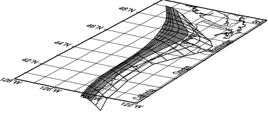
Fig. 3. The geometry of the locked (dark shading) and transition (light shading) zones of the Cascadia subduction fault in the 3-D dislocation model of Fl¨ucket al. (1997). The same model geometry is adopted in the present 3-D viscoelasticfinite element model.
There are three ways to account for the time dependence. (1) The elastic dislocation model can be regarded as a“ snap-shot”at a given time. At a different time during the inter-seismic period, another set of fault-locking parameters may be used to fit the deformation rates then observed. (2) A laboratory-derived rate-dependent friction law can be used to model fault slip in earthquake cycles (e.g., Stuart, 1988). According to this law, the shear resistance along the fault depends on the slip velocity. Velocity-weakening leads to earthquakes; and velocity-strengthening leads to stable slid-ing, analogous to viscousflow. These models usually assume an elastic earth for simplicity, such that the time dependence of crustal deformation is entirely caused by the time depen-dent behavior of the fault. (3) Viscous rock rheology can be taken into account. Although the crust at shallow depths deform elastically in earthquake cycles, it is coupled with the more viscous rocks at greater depths and must show time dependent deformation. This is the approach we use in the present work.
Jameset al. (2000) studied postglacial rebound at northern Cascadia using a detailed ice load model and an earth model consisting of an elastic lithosphere overlying a viscoelastic sublithospheric mantle. Byfitting the model to lake shoreline tilt observations and relative sealevel data, they concluded that the viscosity of the sublithospheric mantle was less than 1020Pa s and likely to be around 1019Pa s, much less than values obtained from global postglacial rebound models that were constrained mostly by data from the continental inte-rior. It is not surprising that the local upper mantle viscosity is low, considering the high heatflow in the arc and backarc region (Blackwellet al., 1990; Lewis, 1991), the high wa-ter content in the subduction zone mantle wedge (Peacock, 1990), and the relatively young age of the subducting Juan de Fuca oceanic plate. As reviewed by Jameset al. (2000), most previous viscoelastic postseismic modeling studies for various subduction zones have found similarly low viscosi-ties.
4.
Model Set-Up
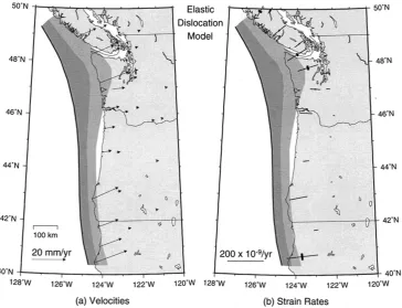
The purpose of the present study is to improve the previous 3-D model by incorporating a viscoelastic rheology. We use exactly the same fault geometry as in the previous 3-D elas-tic dislocation model (Fluck¨ et al., 1997), for a meaningful comparison of results. The shape of the subduction fault and the locked and transition zones in the dislocation model are shown in Fig. 3. Details of the geophysical constraints to the fault geometry were given by Fluck¨ et al. (1997). The width of the locked zone was constrained primarily by thermal lim-its defined by Hyndman and Wang (1993, 1995) but wasfine tuned by Fluck¨ et al.(1997) to provide a betterfit to available leveling data along the Cascadia margin. The results of the elastic dislocation model are reproduced in Fig. 4. The ve-locities, relative to remote model boundaries, are shown only at the continuous GPS sites (see Fig. 1(a)), and the strain rates are shown at the centers of the strain observation networks (see Fig. 1(b)). An observed strain rate is an average over the area of a strain network, and is compared to the model strain rate evaluated at a point at the center of the strain network.
Fig. 4. (a) Velocities relative to remote model boundaries and (b) strain rates predicted by the 3-D elastic dislocation model of Fl¨ucket al. (1997). The velocities are shown at the locations of continuous GPS stations (Fig. 1(a)), and the principal strain rates are shown at the locations of strain observations with a thin bar representing contraction (Fig. 1(b)).
(1997). For northern Cascadia, Wadati-Benioff seismicity allows the slab position to be constrained to 80 km depth, but information about the slab at greater depths and in the rest of the margin comes from low resolution seismic tomog-raphy, as reviewed by Wanget al. (1994). The 3-D slab was constructed by defining downdip geometry along a number of cross-margin profiles and interpolating between these
pro-files. Each individual profile is similar to the 2-D model of Wanget al.(1994). All profiles have the geometry of Fig. 3 at shallow depths, gradually steepen to 60 dip at 200 km, and extend to the bottom of the model at 420 km. Thefinite element mesh, consisting of 46920 nodal points and 42750 eight-node elements, is shown in Fig. 5.
The computer code is written with the aid of the advanced version of the Finite Element Program Generator developed at the Institute of Mathematics, Chinese Academy of Sci-ences (Liang, 1991). The Stabilized Bi-Conjugate Gradient method with the ILUT preconditioner (Axelsson, 1996) cus-tomized for parallel computing is used to solve the large sparse-matrix system. On a dual-processor Ultrasparc-II workstation and with the grid of Fig. 5, one time step takes about 20 minutes, and each run takes 8 to 14 hours. Finite element program output compares well to available two- and three-dimensional surface-loading Maxwell viscoelastic an-alytical solutions (Jameset al., manuscript in preparation). The split-node method of Melosh and Raefsky (1981) is used to prescribe fault slip.
In previous viscoelastic models of earthquake cycles, the effect of gravity was often simulated by applying Winkler restoring forces along the surface (e.g., Cohen, 1994; Wang
et al., 1994). The restoring force works similar to a spring in that the restoring force is proportional to the vertical dis-placement, simulating the material’s tendency to return to the hydrostatic state. Although it allows an accurate calculation of the vertical displacement of the surface, it does not cor-rectly represent the effect of gravity (a body force) within the model. We use an approach, routinely adopted in postglacial rebound modeling, in which the tendency to return to the hydrostatic state is formulated into the governing equation as a pre-stress advection term (e.g., Peltier, 1974). Numeri-cally, it works in a similar way to the Winkler force, but the
“springs”are now imbedded inside the material.
Following Savage (1983), Thatcher and Rundle (1984), Dmowska and Lovison (1988), Cohen (1994), and Taylor et al. (1996), we only consider the fluctuating part of the displacement and stressfields. Steady subduction gives rise to a background stressfield that is constant with time and has no effect on surface deformation unless it exceeds the strength of the crust. Using the same approach as in the elas-tic dislocation model, we assign a backslip rate to the fault to simulate locking, and a forward slip to simulate an earth-quake. Presently constrained by computing time, we model just one great earthquake followed by immediate locking of the fault and the subsequent strain accumulation for several hundred years.
Fig. 5. Thefinite element mesh used in this work. (a) A small portion of the mesh showing detailed structure. (b) The entire mesh.
Fig. 6. Schematic illustration of the fault structure in the viscoelastic model. The rupture zone is assigned a forward slip to simulate earthquake rupture or a backslip rate to simulate interseismic fault locking. The prescribed slip or backslip rate taper to zero over the transition zone. The bebavior of the transition zone is also controlled by the thin viscoelastic layer along it.
sliding part of the fault (Miyashita, 1987; Wanget al., 1994). For simplicity, we let the thin layer have the same mechan-ical properties as the asthenosphere. At the coseismic step, the full-rupture zone is assigned a large slip, and the amount of slip decreases linearly to zero over the transition zone. For the interseismic time step, the rupture zone becomes the locked zone where a backslip rate is assigned. Because of stress relaxation in the viscoelastic thin layer and astheno-sphere, the slip rate of the fault in the transition zone and further downdip is not constant with time, and the downdip
end of the transition zone is not afixed point, as will be shown in the next section.
5.
Model with Uniform Convergence along Strike
In the elastic dislocation model of Fluck¨ et al. (1997), the NUVEL-1 (DeMets et al., 1990) Juan de Fuca–North America (JDF–NA) convergence direction (69◦) and rate (42 mm/yr) at northern Washington was used for the entire Cascadia subduction zone. For comparison, wefirst develop a model using this uniform convergence direction and rate. The effect of along-strike variation of convergence will be discussed in the next section.
We assume a coseismic slip of 20 m for the full-rupture zone of the fault, followed by a backslip rate of 40 mm/yr. The 20 m coseismic slip represents the recovery of all slip deficit accumulated over 500 years in one great earthquake rupture. Paleoseismic studies show that the recurrence inter-val can vary between about 200 and 800 years, and 500 years is a commonly accepted average (Atwater and Hemphill-Haley, 1997). The coseismic deformation of the upper sur-face of the model is essentially a scaled mirror image of the interseismic deformation of the elastic dislocation model (Fig. 4) and is not displayed here. In the elastic dislocation model, which has no time dependence, the coseismic rupture has no effect on subsequent interseismic deformation. In the viscoelastic model, however, the deformation rate at anytime depends on the deformation history, including the effect of the previous earthquake.
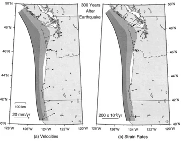
Figures 7(a) and 7(b) illustrate the surface velocities rel-ative tofixed, remote model boundaries and strain rates, re-spectively, 50 years after the great earthquake. Figures 8(a) and 8(b) show the results 300 years after the earthquake. Since the last great Cascadia earthquake occurred 300 years ago (Satakeet al., 1996), the 300-year results represent the present-day deformation. However, because the GPS ve-locities indicate both interseismic and secular deformation, a direct comparison of the 300-year model velocities with GPS velocities is not very meaningful, particularly for central and southern Cascadia. In British Columbia and northern Wash-ington, where there is less secular deformation, the model velocities generally agree with the GPS velocities in magni-tude but not in direction (Fig. 1(a)). The direction depends on the plate convergence model employed and will be discussed in the next section. A comparison between the 50-year and 300-year results indicates a strong time dependence.
Fig. 7. (a) Velocities and (b) principal strain rates (thin bar representing contraction) predicted by the uniform convergence viscoelastic model at 50 years after the great earthquake.
after the 1964Mw =9.2 earthquake (Freymuller, personal communication, 2000) and in South America 40 years after the 1960 Mw = 9.5 Chilean earthquake (Khazaradze, per-sonal communication, 2000). Later in the model interseismic period, the effect of the coseismic deformation diminishes and the effect of fault locking dominates all sites. At 300 years after the earthquake, the model velocity at DRAO is only about 1 mm/yr, a value much less than uncertainties in the GPS velocity vectors, and therefore the model velocties can be compared with the GPS vectors relative to DRAO (Fig. 1(a)). At this time, the asthenosphere is relaxed with respect to the coseismic deformation. Itsfluid-like behav-ior makes it much weaker than a purely elastic medium and hence provides less stress to resist interseismic deformation of the overlying crust. Therefore, elastic interseismic crustal deformation occurs over a broader region from the deforma-tion front than in the elastic dislocadeforma-tion model.
Shown in Fig. 9 is the relative slip of the fault zone across the thin layer (Fig. 6) along a profile across southern Vancou-ver Island. Thefirst 60 km from the deformation front is the locked zone with a prescribed uniform backslip rate (or slip deficit). The transition zone extends to 120 km, overlapping with a viscoelastic layer as shown in Fig. 6. At 50 and 100 years after the earthquake, a segment of the fault landward of the transition zone still slips forward faster than the plate convergence rate, a delayed response to the coseismic defor-mation. At 300 years after the earthquake, the slip distribu-tion is more like what is prescribed in the elastic dislocadistribu-tion model, but there is not a well defined transition zone. Full slip at the plate convergence rate (zero backslip rate) begins not at 120 km but much more landward, effectively giving a wider“transition zone”. This effective transition zone will become even wider as the fault remains locked.
The strong time dependence is also illustrated by the strain rate evolution. Deformation is much faster 50 years after the earthquake (Fig. 7(b)) than 300 years after (Fig. 8(b)). Among the observed strain rates (Fig. 1(b)), the tensor solu-tions have much less uncertainty than the older shear strain estimates and serve better as model constraints. Except near the northern and southern limits of the subduction zone, where the backslip model becomes invalid, both the elastic dislocation model and the 300-year results of the viscoelas-tic modelfit these observations reasonably well, although the
Fig. 9. Backslip rates of the fault for the uniform convergence viscoelastic model along a profile across southern Vancouver Island.
former tends to overestimate the strain rates (Fig. 4(b)). Be-cause elastic interseismic crustal deformation occurs over a broader region in the viscoelastic model, velocity decreases landward at a slower rate, resulting in lower strain rates.
Using different viscosity values changes the time-scale of the deformation. If we use a viscosity of 1020 Pa s (results not shown), the system behaves basically elastically over a 500 year earthquake interval. The postseismic seaward motion of the inland sites, as well as their landward motion 300 years after the earthquake, is very small. At 300 years, the landward decrease of predicted velocities is faster, and hence the strain rates are larger, similar to the prediction of the elastic dislocation model. The smaller strain rates predicted using a viscosity of 1019 Pa s are in a better agreement with the observations. For a lower viscosity of 5×10¹⁸ Pa s (results not shown), the time dependent behavior is more pronounced. The seaward motion of inland sites at 50 years is faster, and the landward velocity decrease at 300 years is more gradual.
6.
Model with Variable Convergence along Strike
In this section, we consider a model in which the con-vergence direction and speed vary along strike. According to the NUVEL-1 plate model (DeMets et al., 1990), Juan de Fuca–North America (JDF–NA) convergence is nearly
Table 1. Juan de Fuca–North America Euler poles.
Name Latitude Longitude Rotation Rate∗ Reference
Riddihough 29.40 −111.70 −1.09 Riddihough (1984)
NUVEL-1 20.70 −112.20 −0.80 DeMetset al. (1990)
Wilson 31.60 −116.40 −1.26 Wilson (1993)
NUVEL-1A 23.28 −112.04 −0.82 DeMetset al. (1994)
New Pole† 26.63 −110.45 −0.80 DeMets and Dixon (1999) ∗Rotation rate is in Degrees/Ma.
†This pole was determined using the GPS constrained JDF–NA pole of DeMets and Dixon (1999) and the
JDF–Pacific pole reported in DeMetset al. (1994) based on the results of Wilson (1993).
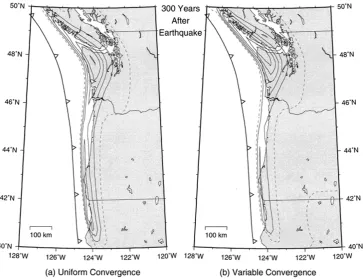
Fig. 11. (a) Velocities and (b) principal strain rates (thin bar representing contraction) predicted by the variable convergence viscoelastic model at 300 years after the great earthquake.
margin-normal off northern British Columbia, but to the south the convergence direction becomes more oblique and the convergence rate becomes smaller (Fig. 10). For simplic-ity, the variation of the convergence direction and rate was neglected in the 3-D dislocation model of Fluck¨ et al. (1997). In addition, there appears to be a great deal of uncertainty in the position of the Euler pole of JDF–NA motion. Table 1 lists various published JDF–NA pole positions and rotation rates. The JDF–NA pole determined by Riddihough (1984) leads to more oblique convergence for the entire margin and more pronounced along-strike variations of the convergence direction and rate as compared to NUVEL-1. Milleret al. (2001) and McCaffreyet al. (2000) both used a JDF–NA pole derived from a Pacific-NA pole newly determined by DeMets and Dixon (1999) and the Pacific–JDF pole of NUVEL-1a (DeMetset al., 1994; Wilson, 1993). This most recent pole predicts a convergence pattern very similar to that predicted
by Riddihough, but with smaller convergence rates (Fig. 10). We have used Riddihough’s pole for our test of the effect of along-strike variable plate convergence. As in the previ-ous model, we ignore triple-junction related complications in the regions near the northern and southern termini of the subduction zone.
Fig. 12. Uplift rates at 300 year after the great earthquake for (a) the uniform convergence model and (b) the variable convergence model. The contour interval is 1 mm/yr, and the dashed line is the zero contour line.
contraction. The distance between southern Cascadia and DRAO is shortened as indicated by the predicted velocities, but the rate of the“margin-parallel”contraction is much less than the rate of the“margin-normal”contraction.
There are two interpretations for the predicted“ margin-parallel”contraction. (1) It is part of the elastic interseismic deformation. If this is the case, a major part of the north-ern component of the GPS velocities in southnorth-ern Cascadia reflects the elastic deformation. This interpretation leads to speculations regarding whether the fault slips in exactly the opposite direction during a great earthquake to recover all the elastic deformation. If the earthquake slip vector is less oblique, the unrecovered part of the margin-parallel shorten-ing will have to be converted into the secular, permanent shortening or translation of the forearc. This provides a mechanism for the coupling of earthquakes and forearc defor-mation over many great earthquake intervals. (2) The model may incorrectly incorporate part of the secular deformation of the forearc as interseismic deformation. In other words, the margin-parallel shortening and its driving mechanism should have been subtracted from both the data and model parame-ters in thefirst place. For example, if the secular deformation of the forearc is known a priori, a correction can be made to the plate convergence model such that it is the JDF–forearc, instead of JDF–NA, convergence that is used to define model parameters. The modeled deformation will then be free of the secular effect. We have done some preliminary tests us-ing the kinematic forearc deformation model of Wellset al. (1998) and the new JDF–NA pole derived from the results of DeMets and Dixon (1999) or Riddihough’s pole (1984). Interestingly but fortuitously, the resultant JDF–forearc
con-vergence along the central and southern Cascadia margin is very similar to the uniform convergence model assumed in the model of Fluck¨ et al. (1997).
The two interpretations are two end-member cases cor-responding to the two possible driving mechanisms for the margin-parallel compressive stress in the Cascadia forearc hypothesized by Wang (1996). Thefirst interpretation is an illustration of the subduction driving mechanism, in which the margin-parallel component of oblique subduction causes margin-parallel compression in the Cascadia forearc“sliver”
whose leading edge is buttressed by the Canadian Coast Mountains. The second interpretation requires the forearc to be pushed from its trailing edge by Sierra Nevada, regard-less of the subduction process. Wang (1996) suggested that the margin-parallel compression in the Cascadia forearc ap-peared to be the result of the combination of both. From a purely kinematic point of view, the second interpretation above is more appealing because of its simplicity.
7.
Vertical Displacements
The dislocation model of Fluck¨ et al. (1997) was con-strained by vertical deformation data such as leveling and tide gauge measurements. Here we have focused on the horizontal deformation data and model results. It is use-ful to compare the vertical displacements predicted by our 3-D viscoelastic models with those predicted by the 3-D elastic dislocation model. Figure 12 shows the uplift rates 300 years after the great earthquake predicted by both the and variable-convergence models. The uniform-convergence model (Fig. 12(a)) and the dislocation model predict similar results (seefigure 4 of Fluck¨ et al., 1997). The variable-convergence viscoelastic model predicts lower uplift rates along the Oregon coast but higher rates along the coast of British Columbia. In the model, oblique subduction causes a coast-parallel motion and a“piling up”of materials at the corner of the subduction zone in northern Washington and southern British Columbia. It is presently unclear how the uplift at this corner is affected and limited by secular geo-logical deformation and how the process should be modeled. Like the horizontal velocities, the uplift rates approximately scale with the convergence rate used, and using the most re-cently determined JDF–NA pole (Table 1) will lead to lower convergence rates and hence lower uplift rates. Finally, our sensitivity tests indicate that the uplift rates are affected by the thickness of the oceanic plate much more than the hori-zontal velocities are. Unlike the uniform elastic half-space assumed in the dislocation model, the interaction between the elastic lithosphere and viscoelastic asthenosphere gives rise to a slight, time dependent, plate bending effect that depends on plate thickness. Further research is required to understand vertical deformation in a viscoelastic model.
8.
Summary
We have constructed a 3-D viscoelastic finite element model for the interseismic deformation of the Cascadia sub-duction zone. The model consists of elastic lithospheric plates, including the slab, and a uniform viscoelastic as-thenosphere. A low viscosity of 1019 Pa s, as constrained by a recent postglacial rebound analysis, is assumed for the asthenosphere. The geometry of the subducting plate is an extension of those used in a previous 3-D elastic dislocation model and a 2-D viscoelasticfinite element model.
Prescribed backslip rates are used, after an initial coseis-mic rupture, to simulate the effect of the interseiscoseis-mically locked subduction fault. The geometry of the rupture zone is copied exactly from the previous 3-D dislocation model, but a thin viscoelastic layer is introduced along the fault surface to allow a natural transition from the locked zone and the viscoelastic asthenosphere further downdip. Because of the simplicity of the rheological model, the results are of a pre-liminary nature. Nevertheless, they raise some fundamental issues that will provide guidance for future modeling and experiments.
The model with a uniform plate convergence direction and rate is very similar to the previous 3-D dislocation model ex-cept for the viscoelastic rheology. The most important effect of introducing viscoelasticity is the time dependence of the interseismic deformation. The interseismic deformation is the combined effect of the previous great earthquake and
the subsequent loading of the locked fault. Shortly after the earthquake, the deformation is dominated by postseismic re-laxation. A part of the fault downdip from the rupture zone may slip forward aseismically at a rate faster than the plate convergence speed, giving rise to seaward motion of some inland sites and large strain rates. Later in the interseismic period, the deformation is dominated by fault locking alone. Because of the relaxation of the asthenosphere, elastic de-formation takes place over a broader region of the overriding plate than assumed in the elastic dislocation model, and hence the forearc strain rates 300 years after the great earthquake are less than those in the dislocation model. We have demon-strated these effects using results 50 and 300 years after the previous earthquake, but the reader should be reminded that the exact timing of the various behaviors depends on the de-tails of the rheology. For example, if a stress dependent (non-linear) viscosity is used for the thin layer along the fault, or a rate dependent friction law (also nonlinear) is used, the du-ration of the postseismic deformation will be much shorter. However, the backslip approach will no longer be valid if nonlinearity is involved, because the “steady plate conver-gence”cannot be readily subtracted from the total deforma-tionfield. The prominence of the postseismic deformation also depends on the size of the previous earthquake. If the coseismic fault slip 300 years ago was 10 m instead of 20 m, the effect of the postseismic deformation should be reduced by half.
We have also constructed a model with a variable conver-gence direction and rate along strike. The JDF–NA Euler pole determined by Riddihough (1984) is used, which re-sults in a convergence pattern very similar to what is pre-dicted from the most recent plate motion estimates. Model predicted strain rates 300 years after the earthquake in both the uniform and variable convergence models agree with the geodetically determined contemporary strain rates. The pre-dicted velocities at this time roughly scale with the plate convergence rate. If plate convergence rates from the most recent JDF–NA pole (Fig. 10) are used, the velocities will be about 20% smaller. The variable convergence model il-lustrates the effect of strain partitioning. The margin-normal component of plate convergence is largely responsible for the interseismic elastic contraction of the forearc in the nearly margin-normal direction. The margin-parallel component results in a shear deformation further inland. Associated with this shear deformation is a slight shortening of the fore-arc along-strike. This shortening appears as elastic deforma-tion in the model, but it may be more reasonable for it to be modeled as permanent deformation.
Acknowledgments. We thank G. Liang, Chinese Academy of Sci-ences, for his leading role in the development of the Finite Element Program Generator which was used to develop the computer code in this study. D. D. Jackson and T. Kato provided valuable reviews. Geological Survey of Canada contribution 2000181.
References
Atwater, B. F. and E. Hemphill-Haley, Recurrence intervals for great earth-quakes of the past 3500 years at northeastern Willapa Bay, Washington, U.S.Geological Survey Professional Paper,1576, 108 pp., 1997. Axelsson, O.,Iterative Solution Methods, 654 pp., Cambridge University
Press, Cambridge, 1996.
Washington and thermal conditions in the Cascade Range,J. Geophys. Res.,95, 19,495–19,516, 1990.
Cohen, S. C., Evaluation of the importance of model features for cyclic deformation due to dip-slip faulting,Geophys. J. Int.,119, 831–841, 1994.
DeMets, C. and T. H. Dixon, New kinematic models for Pacific-North Amer-ica motion from 3 Ma to present, I: Evidence for steady motion and biases in the NUVEL-1A model,Geophys. Res. Lett.,26, 1921–1924, 1999. DeMets, C., R. G. Gordon, D. F. Argus, and S. Stein, Current plate motions,
Geophys. J. Int.,101, 425–478, 1990.
DeMets, C., R. G. Gordon, D. F. Argus, and S. Stein, Effects of recent revisions to the geomagnetic reversal time scale on estimates of current plate motions,Geophys. Res. Lett.,21, 2191–2194, 1994.
Dmowska, R. and L. C. Lovison, Intermediate-term seismic precursors for some coupled subduction zones,Pure Appl. Geophys.,126, 643–664, 1988.
Douglass, J. J. and B. A. Buffett, The stress state implied by dislocation models of subduction deformation,Geophys. Res. Lett.,22, 3115–3118, 1995.
Dragert, H., Recent horizontal strain accumulation on Vancouver Island, British Columbia (abstract),Eos Trans. AGU,72, Fall meeting suppl., 314, 1991.
Dragert, H. and M. Lisowski, Crustal deformation measurements on Van-couver Island, British Columbia: 1976 to 1988, inGlobal and Regional Geodynamics, edited by P. Vyskocil, C. Reigber, and P. A. Cross, 349 pp., Springer-Verlag, New York, 1990.
Dragert, H., R. D. Hyndman, G. C. Rogers, and K. Wang, Current defor-mation and the width of the seismogenic zone of the northern Cascadia subduction thrust,J. Geophys. Res.,99, 653–668, 1994.
Dragert, H., X. Chen, and J. Kouba, GPS monitoring of crustal strain in Southwest British Columbia with the Western Canada Deformation Ar-ray,Geomatica,49, 301–313, 1995.
Fl¨uck, P., R. D. Hyndman, and K. Wang, Three-dimensional dislocation model for great earthquakes of the Cascadia subduction zone,J. Geophys. Res.,102, 20,539–20,550, 1997.
Harris, R. N. and D. S. Chapman, A comparison of mechanical thickness estimates from trough and seamount loading in the southeastern Gulf of Alaska,J. Geophys. Res.,99, 9297–9317, 1994.
Henton, J. A., GPS Studies of Crustal Deformation in the Northern Cascadia Subduction Zone, Ph.D. thesis, University of Victoria, 169 pp., British Columbia, 2000.
Henton, J. A., H. Dragert, R. D. Hyndman, and K. Wang, Geogetic moni-toring of crustal deformation and strain on Vancouver Island (abstract),
Eos Trans. AGU,80, Fall meeting suppl, F276, 1999.
Hyndman, R. D. and K. Wang, Thermal constraints on the zone of major thrust earthquake failure, The Cascadia subduction zone,J. Geophys. Res.,98, 2039–2060, 1993.
Hyndman, R. D. and K. Wang, Current deformation and thermal constraints on the zone of potential great earthquakes on the Cascadia subduction thrust,J. Geophys. Res.,100, 22,133–22,154, 1995.
James, T. S., J. J. Clague, K. Wang, and I. Hutchinson, Postglacial rebound at the northern Cascadia subduction zone,Quat. Sci. Rev.,19, 1527–1541, 2000.
Khazaradze, G., A. Qamar, and H. Dragert, Tectonic deformation in western Washington from continuous GPS measurements,Geophys. Res. Lett.,
26, 3153–3156, 1999.
Lewis, T., Heatflux in the Canadian Cordillera, inNeotectonics of North America, edited by D. B. Slemmons, E. R. Engdahl, M. D. Zoback, and D. D. Blackwell, 498 pp., Geological Society of America, Boulder, Colorado, 1991.
Liang, G. P., Finite element program generator andfinite element language, inReliability and Robustness of Engineering Software II, edited by C. A. Brebbia and A. J. Ferrante, 385 pp., Computational Mechanics Publica-tions, London, 1991.
McCaffrey, R., M. D. Long, C. Goldfinger, P. C. Zwick, J. L. Nabelek, C. K. Johnson, and C. Smith, Rotation and plate coupling along the southern Cascadia subduction zone,Geophys. Res. Lett.,27, 3117–3120, 2000.
Melosh, H. J. and A. Raefsky, A simple and efficient method for introducing faults intofinite element computations,Bull. Seismol. Soc. Am.,71, 1391– 1400, 1981.
Miller, M. M., D. J. Johnson, C. M. Rubin, H. Dragert, K. Wang, A. Qamar, and C. Goldfinger, GPS-determination of along-strike variation in Casca-dia margin kinematics: Implications for relative plate motion, subduction zone coupling, and permanent deformation,Tectonics, 2001 (in press). Miyashita, K., A model of plate convergence in Southwest Japan, inferred
from levelling data associated with the 1946 Nankaido earthquake, J. Phys. Earth,35, 449–467, 1987.
Murray, M. H. and M. Lisowski, Strain accumulation along the Cascadia subduction zone,Geophys. Res. Lett.,27, 3631–3634, 2000.
Peacock, S. M., Fluid processes in subduction zones,Science,248, 329–337, 1990.
Peltier, W. R., The impulse response of a Maxwell Earth,Rev. Geophys. Space Phys.,12, 649–668, 1974.
Pezzopane, S. K. and R. J. Weldon, II, Tectonic role of active faulting in central Oregon,Tectonics,12, 1140–1169, 1993.
Riddihough, R., Recent movements of the Juan de Fuca plate system,J. Geophys. Res.,89, 6980–6994, 1984.
Satake, K., K. Shimazaki, Y. Tsuji, and K. Ueda, Time and size of a giant earthquake in Cascadia inferred from Japanese tsunami records of January 1700,Nature,378, 246–249, 1996.
Savage, J. C., A dislocation model of strain accumulation and release at a subduction zone,J. Geophys. Res.,88, 4984–4996, 1983.
Savage, J. C., Comment on“The stress state implied by dislocation models of subduction deformation”by J. J. Douglass and B. A. Buffett,Geophys. Res. Lett.,23, 2709–2710, 1996.
Savage, J. C., M. Lisowski, and W. H. Prescott, Strain accumulation in western Washington,J. Geophys. Res.,96, 14,493–14,507, 1991. Savage, J. C., J. L. Svarc, W. H. Prescott, and M. H. Murray,
Deforma-tion across the forearc of the Cascadia subducDeforma-tion zone at Cape Blanco, Oregon,J. Geophys. Res.,105, 3095–3120, 2000.
Stuart, W. D., Forecast model for great earthquakes at the Nankai Trough subduction zone,Pure Appl. Geophys.,126, 619–641, 1988.
Taylor, M. A., G. Zheng, J. R. Rice, W. D. Stuart, and R. Dmowska, Cyclic stressing and seismicity at strongly coupled subduction zones,J. Geophys. Res.,101, 8363–8381, 1996.
Thatcher, W., The earthquake deformation cycle at the Nankai Trough, Southwest Japan,J. Geophys. Res.,89, 3087–3101, 1984.
Thatcher, W. and J. B. Rundle, A viscoelastic coupling model for the cyclic deformation due to periodically repeated earthquakes at subduction zones,
J. Geophys. Res.,89, 7631–7640, 1984.
Wang, K., Simplified analysis of horizontal stresses in a buttressed forearc sliver at an oblique subduction zone,Geophys. Res. Lett.,23, 2021–2024, 1996.
Wang, K., Stress-strain“paradox”, plate coupling, and forearc seismicity at the Cascadia and Nankai subduction zones,Tectonophys.,319, 321–338, 2000.
Wang, K. and J. He, Mechanics of low-stress forearcs: Nankai and Cascadia,
J. Geophys. Res.,104, 15,191–15,205, 1999.
Wang, K. and K. Suyehiro, How does plate coupling affect crustal stresses in Northeast and Southwest Japan?,Geophys. Res. Lett.,26, 2307–2310, 1999.
Wang, K., H. Dragert, and H. J. Melosh, Finite element study of uplift and strain across Vancouver Island,Can. J. Earth Sci.,31, 1510–1522, 1994. Wang, K., T. Mulder, G. C. Rogers, and R. D. Hyndman, Case for very low coupling stress on the Cascadia subduction fault,J. Geophys. Res.,100, 12,907–12,918, 1995.
Wells, R. E., C. S. Weaver, and R. J. Blakely, Forearc migration in Cascadia and its neotectonic significance,Geology,26, 759–762, 1998. Wilson, D. S., Confidence intervals for motion and deformation of the Juan
de Fuca plate,J. Geophys. Res.,98, 16,053–16,071, 1993.