R E S E A R C H
Open Access
Motion parameter estimation of multiple
ground moving targets in multi-static passive
radar systems
Saurav Subedi
1, Yimin D Zhang
1*, Moeness G Amin
1and Braham Himed
2Abstract
Multi-static passive radar (MPR) systems typically use narrowband signals and operate under weak signal conditions, making them difficult to reliably estimate motion parameters of ground moving targets. On the other hand, the availability of multiple spatially separated illuminators of opportunity provides a means to achieve multi-static diversity and overall signal enhancement. In this paper, we consider the problem of estimating motion parameters, including velocity and acceleration, of multiple closely located ground moving targets in a typical MPR platform with focus on weak signal conditions, where traditional time-frequency analysis-based methods become unreliable or infeasible. The underlying problem is reformulated as a sparse signal reconstruction problem in a discretized parameter search space. While the different bistatic links have distinct Doppler signatures, they share the same set of motion parameters of the ground moving targets. Therefore, such motion parameters act as a common sparse support to enable the exploitation of group sparsity-based methods for robust motion parameter estimation. This provides a means of combining signal energy from all available illuminators of opportunity and, thereby, obtaining a reliable estimation even when each individual signal is weak. Because the maximum likelihood (ML) estimation of motion parameters involves a multi-dimensional search and its performance is sensitive to target position errors, we also propose a technique that decouples the target motion parameters, yielding a two-step process that sequentially estimates the acceleration and velocity vectors with a reduced dimensionality of the parameter search space. We compare the performance of the sequential method against the ML estimation with the consideration of imperfect knowledge of the initial target positions. The Cramér-Rao bound (CRB) of the underlying parameter estimation problem is derived for a general multiple-target scenario in an MPR system. Simulation results are provided to compare the performance of the sparse signal reconstruction-based methods against the traditional time-frequency-based methods as well as the CRB.
Keywords: Multi-static passive radar; Sparse reconstruction; Group sparsity; Motion parameter estimation
1 Introduction
Multi-static passive radar (MPR) has recently attracted significant research interests primarily due to its low cost and covertness compared to a conventional radar system. Also, since passive radar systems use signals of opportunity as transmitters, they do not exacer-bate the problem of spectral congestion [1]. MPR sys-tems are typically characterized by low signal power,
*Correspondence: [email protected]
1Center for Advanced Communications, Villanova University, Villanova, PA 19085, USA
Full list of author information is available at the end of the article
narrow signal bandwidth, bistatic mode of operation, and availability of multiple spatially separated trans-mitters, rendering them significantly different from conventional radar systems. From a signal process-ing perspective, operation in low signal-to-noise ratio (SNR) conditions exploiting narrowband signals creates additional challenges for target detection, localization, and tracking. On the other hand, availability of sev-eral spatially separated illuminators can be exploited to achieve a higher effective SNR and multi-static diversity [2].
Motion parameter estimation of ground moving tar-gets has been studied extensively in the context of
conventional radar systems (e.g., single-antenna radar [3], phased-array radar [4], and input multiple-output (MIMO) radar [5-7]). Several advanced signal processing techniques, including time-frequency analysis, motion compensation, and range migration compensa-tion (e.g., [8-10]), have been developed for the detec-tion and parameter estimadetec-tion of moving targets based on their Doppler signatures. However, limited work has been done in estimating target motion parameters in MPR systems (e.g., [11,12]). In this paper, we inves-tigate the problem of motion parameter estimation of ground moving targets in a multi-static passive airborne radar.
Existing motion parameter estimation techniques (e.g., [13-15]) are based on time-frequency analysis of Doppler signatures of received signals, which are commonly mod-eled as general-order polynomials [16]. For a moder-ately long coherent processing interval (CPI), it suffices to model the target motion by a second-order polyno-mial or a linear frequency-modulated signal. As such, time-frequency analysis methods are used to estimate the chirp parameters followed by a mapping to the actual target motion parameters. When multiple targets are present, the Doppler signature of the radar return is modeled as a linear sum of multiple chirp signals [17].
In low SNR situations, as encountered in typical MPR systems, reliable estimation of chirp parameters for each bistatic link may become difficult. As such, it is desirable to enhance the overall signal quality either by extending the CPI or by exploiting the availability of multiple bistatic links. The state of the art for estimating motion parame-ters of closely spaced multiple ground moving targets in typical MPR systems is incomplete, because of the rather non-trivial two issues:
1. Since the Doppler signature corresponding to each bistatic link cannot be reliably estimated, and it is rather difficult to directly combine them in the time-frequency domain for overall signal enhancement, traditional methods based on time-frequency analysis cannot effectively benefit from the availability of multiple transmitters. 2. Although a longer CPI can be used to enhance
the SNR corresponding to each bistatic link, the target range migration must be compensated for before processing the signal over the azimuthal time. A longer CPI, however, requires the consideration of higher-order motion parameters (e.g., acceleration and jerk) which are more difficult to estimate and compensate. This further limits the applicability of time-frequency analysis-based methods, particulary for highly accelerating (or decelerating) targets.
A motion parameter estimation method based on sparse signal reconstruction has recently been developed [2], which coherently combines data from all available illumi-nators of opportunity and, thereby, achieves overall sig-nal enhancement and multi-static diversity. This method involves a sequential estimation process, where the tar-get acceleration is estimated by coherently fusing all the signal observations mapped into the ambiguity func-tion of the respective Doppler signature and detecting the combined peak via a direct search. The estimated value of target acceleration is then used in the estima-tion of the target velocity by exploiting sparse signal reconstruction. However, the applicability of this method is limited to a single-target scenario. Multiple closely spaced targets may be frequently encountered in MPR systems due to the small signal bandwidth and the cor-responding poor range resolution. A method based on exhaustive search becomes computationally inefficient for such a multiple-target scenario because its computational complexity increases exponentially with the number of targets.
parame-ter estimation of two closely located ground moving targets.
The rest of the paper is organized as follows. Section 2 formulates the signal model for the Doppler signature in a multi-target scenario considering a multi-static pas-sive radar network configuration. Section 3 presents the motion parameter estimation algorithms, including a brief review of the time-frequency analysis-based method and the description of the proposed techniques that are based on maximum likelihood (ML) and sequential estimations, both exploiting the group sparsity of target motion param-eters. The effect of imperfect knowledge of the initial target positions on the motion parameter estimation is also examined in Section 3. Section 4 derives the CRB for the underlying parameter estimation problem. Section 5 presents simulation results that compare the estimation accuracy of the ML and sequential estimation methods against the CRB as well as the traditional time-frequency analysis-based methods. Finally, conclusions are drawn in Section 6.
The following notations are used in this paper. A lower (upper) case bold letter denotes a vector (matrix). In par-ticular,IN denotes theN ×N identity matrix.(.)∗,(.)T,
and(.)H, respectively, denote complex conjugation, trans-pose, and Hermitian operations.·1and·, respectively, denote thel1 andl2 norm of a vector, whereas(.)and (.), respectively, stand for the real part of a complex number, andCN(a,b)denotes standard complex normal distribution with mean a and variance b. In addition, diag(.) and tr(.), respectively, denote the diagonal and trace operations.
2 Signal model
2.1 Geographical relationship
We consider a problem of estimating motion parameters of multiple, closely located, ground moving targets in a typical MPR system. We assume that the MPR system operates in a multiple-frequency network, i.e.,N broad-cast stations, located at b(n), n = 1,. . .,N, transmit waveforms in non-overlapping frequency bands which are respectively centered at f(n), n = 1,. . .,N. These sta-tions are assumed stationary and their locasta-tions precisely knowna priori.
An airborne receiver, initially located atr0, is assumed to
be moving along its track direction with a uniform veloc-ityvr, whereas there areKclosely located ground moving
targets. Thekth target is assumed to be initially located at
p(0k), moving with an initial velocity ofv(k)and an acceler-ation ofa(k). Because only ground targets are considered, thez-axis components ofp(0k),v(k), anda(k)are assumed to be zero.
The direct range between the nth illuminator and the receiver, corresponding to the reference channel, is defined as
r(n)(t)= r(t)−b(n), (1)
where r(t) = r0 +vrt represents the trajectory of the
receiver at time t. Likewise, the bistatic range between the nth transmitter, the kth target, and the receiver is expressed as
ρ(n,k)(t)= p(k)(t)−b(n) + p(k)(t)−r(t), (2)
where p(k)(t) = p(0k) + v(k)t + 12a(k)t2 represents the
trajectory of thekth target at timet.
2.2 Reference and surveillance signals
The direct path signal received from thenth transmitter can be expressed as
s(rn)(t)=u(n)
t−r(n)(t)/c
exp
−j2πf(n)r(n)(t)/c
+η(n)
r (t),
(3)
where the subscript ‘r’ represents the reference chan-nel, u(n)(t) is the baseband representation of the signal transmitted from the nth illuminator, c is the veloc-ity of wave propagation, and ηr(t) represents the
addi-tive noise. Since passive radars use broadcast signals, it can be assumed that the transmitted signal is per-fectly reconstructed at the receiver after demodulation and forward error correction [18]. Therefore, the direct path signal, after reconstruction and error correction, becomes
s(rn)(t)=u(n)(t−r(n)(t)/c)exp−j2πf(n)r(n)(t)/c,
(4)
which is used as the reference signal.
The surveillance signal reflected from the kth target corresponding to the signal transmitted by thenth illumi-nator is
s(sn,k)(t)=σ(n,k)u(n)t−ρ(n,k)(t)/c
×exp−j2πf(n)ρ(n,k)(t)/c+ηs(n)(t), (5)
where the subscript ‘s’ denotes the surveillance channel, σ(n,k)is the target reflection coefficient corresponding to
thekth target, andηs(n)(t)is the additive noise.
filter output. The phase term of the output of the matched filter is determined by the difference between the bistatic transmitter-target-receiver range and the direct transmitter-receiver range. Denote t as the azimuthal sampling interval used in the matched filtering, andtm =
mt be the azimuthal sampling instants, m = 0,. . ., M−1. Then, the range difference at themth azimuthal sampling instant,tm, can be expressed as
R(n,k)(tm)=ρ(n,k)(tm)−r(n)(tm)
=p(0k)+v(k)tm+a(k)tm2/2−b(n)
+p(0k)+v(k)tm+a(k)tm2/2−r0−vrtm
−r0+vrtm−b(n).
(6)
From (6), it can be inferred that motion of ground mov-ing targets and motion of the radar platform are the two sources of range migration. In view of a typical MPR system, due to the narrow signal bandwidth and, con-sequently, the low bistatic range resolution, target range migration is not a critical issue for a short or moder-ate CPI. However, when an extended CPI is required, e.g., in very weak signal conditions, target range migra-tion must be properly compensated for. The commonly used range migration compensation methods, such as the Keystone transform [19], can be used to compensate for the linear range migration. However, when accelera-tion and higher order moaccelera-tion parameters are prominent features of the target motion, target range migration compensation emerges as a challenging problem. In the underlying problem, we consider a moderately long CPI, which obviates the need for target range migration compensation.
On the other hand, since motion parameters of the receiver platform are precisely known, we can compensate for the range migration due to its movement [15] about a ground reference position in close vicinity of the actual position of targets, referred to as scene origins. For thekth target, considering a scene origin atq(k), the bistatic range between the nth transmitter, the scene origin, and the receiver can be calculated at themth azimuthal sampling instant as
ζ(n)(t
m)= q(k)−b(n) + q(k)−r(tm). (7)
Therefore, after compensating for the range migration due to the movement of the receiver platform, the range difference at azimuthal timetmcan be expressed as
˜
R(n,k)(tm)=ρ(n,k)(tm)−ζ(n,k)(tm)
=p(k)(tm)−b(n)+p(k)(tm)−r(tm)
−q(k)−b(n)−q(k)−r(tm)
=p(0k)+v(k)tm+a(k)t2m/2−b(n)
+p(0k)+v(k)tm+a(k)t2m/2−r0−vrtm
−q(k)−b(n)−q(k)−r0−vrtm.
(8)
2.4 Observed Doppler signature
The signal transmitted by each of the N illuminators is reflected by the K moving targets, and hence, the sig-nal arriving at the receiver is the superposition of radar returns from the K targets. Thus, the output of the receiver matched filter at azimuthal timetm
correspond-ing to the nth illuminator, after range migration com-pensation due to the motion of the receiver platform at the scene origin, can be expressed as a linear sum of K different Doppler signatures,
s(n)(tm)= K
k=1
ξ(n,k)expj2πf(n)R˜(n,k)(t m)/c
+η(n)(t m),
(9)
where ξ(n,k) = ξR(n,k) + jξI(n,k) is a complex num-ber representing the magnitude of the matched fil-ter output corresponding to the return from the kth target, and η(n)(tm) is the additive Gaussian white
noise output. The complex magnitude ξ(n,k) can be assumed time-invariant because the target radar cross-section (RCS) for a given bistatic pair does not fluc-tuate significantly over the given observation period. Note that the unknown initial phase component due to the complex target reflectivity σ(n,k) is absorbed in the
unknown complex magnitude ξ(n,k). The phase term of
the matched filter output, as discussed in the preceding section, is determined by the range difference, depicted in (8).
Considering a moderately long CPI, the Doppler signa-ture from each target can be modeled as a second-order phase polynomial signal, or referred to as a linear chirp. That is, the phase term ofs(n,k)(tm), denoted asφ(n,k)(tm),
follows a quadratic relationship:
φ(n,k)(t
m)=φ0(n,k)+2πf( n,k)
0 tm+πβ(n,k)t2m, (10)
3 Motion parameter estimation
In this section, we analyze the motion parameter esti-mation of multiple ground moving targets in the given multi-static passive network configuration using the time-frequency analysis and group sparsity-based signal recon-struction method.
3.1 Motion parameter estimation using time-frequency analysis
As described in Section 2, the Doppler signature corre-sponding to a ground moving target can be modeled as a linear chirp for a moderate CPI. The chirp parameters, i.e., the initial frequency and chirp rate, can be estimated using time-frequency analysis techniques such as the Radon-Wigner transform, the fractional Fourier transform (FrFT), and the chirp-Fourier transform. These meth-ods have been widely used in various radar applications (e.g., [20-24]). A motion parameter estimation method, for single as well as multiple closely located ground moving targets, is proposed in [15]. The method proposed in [15] assumesa prioriknowledge of Doppler signature parame-ters corresponding to all bistatic links, obtained using the time-frequency analysis, to estimate motion parameters using
f0(n,k) β(n,k)
=A(n,k)
q(k) v
(k)
a(k) , (11)
where f0(n,k)andβ(n,k), respectively, are the initial Doppler frequency and the chirp rate observed in the signature corresponding to the nth transmitter and target motion parameters v(k) and a(k) of the kth target. The matrix
A(n,k)(q(k)), which maps the chirp parameters to the respective motion parameter, is defined as
A(n,k)
q(k)
= λ1(n)
⎡ ⎢ ⎢ ⎣
q(k)−b(n)
T
q(k)−b(n) +
q(k)−r0
T
q(k)−r0 0
− 2vT r
q(k)−r0
q(k)−b(n)T q(k)−b(n) +
q(k)−r
0 T
q(k)−r0
⎤ ⎥ ⎥
⎦,
(12)
whereλ(n)is the wavelength of the signal corresponding to the thenth transmitter. ForNspatially separated trans-mitters, we obtain 2N distinct equations. Therefore, the four unknown motion parameters of each target can be unambiguously estimated whenN≥2.
However, under weak signal conditions, it is difficult to obtain reliable chirp parameter estimations using time-frequency analysis of the Doppler signatures. In the pres-ence of additive white Gaussian noise, the chirp parameter estimation process exhibits a threshold effect in the sense that, when SNR is below a certain threshold, there is a rapid performance degradation [24]. As discussed earlier,
despite the availability of several transmitters, the Doppler signatures corresponding to different bistatic links are dis-tinct in general and thus cannot be directly combined in the time-frequency domain to improve the estimation reliability and accuracy of the chirp parameters in each bistatic pair.
In the following, we consider exploiting the group sparsity-based signal reconstruction for motion parame-ter estimation. This helps achieve overall signal enhance-ment by combining information from all possible bistatic links and, thereby, obtaining a reliable motion parameter estimation even in weak signal conditions.
3.2 Motion parameter estimation using sparse signal reconstruction
In (8), we see that the motion of a target is determined by four unknown motion parameters, i.e., thex- andy -axis components of its acceleration and velocity. With the a prioriinformation that Doppler signatures correspond-ing to different bistatic links share the same set of motion parameters, the problem can be modeled as a group sparse signal reconstruction problem.
In the underlying problem, the measurement matrix needs to represent a discretized four-dimensional (4-D) space of the unknown motion parameters, such that each point in the discretized space represents a hypothetical combination of target motion parameters(vx,vy,ax,ay). It
is noted that the true motion parameters can assume any value in the continuous space and an attempt to repre-sent the motion parameters in a discretized 4-D space may result in an ‘off-grid’ problem. However, by adequately sampling the parameter space, a good performance can be achieved as long as the mutual coherence among the columns of the measurement matrix is low enough to per-mit the sparse signal reconstruction. The performance of the sparsity-based signal reconstruction method can be improved by increasing the resolution of the measure-ment matrix. However, this increases a risk of increasing the mutual coherence among the columns of the dic-tionary matrix to an extent where sparse reconstruction becomes impractical or infeasible. Considering these two issues, it is important to define the measurement matrix as fine as possible provided that the sparse reconstruction is feasible. Mathematically, it is possible to obtain a joint estimation of multiple-target motion parameters through an ML search.
3.2.1 Maximum likelihood estimation
The N ×1 received signal vector at themth azimuthal sampling instant,tm, can be formed as
s(tm)=
s(1)(tm),s(2)(tm),· · ·,s(N)(tm)
T
=γ(tm)+η(tm),
wheres(n)(tm)is the output of the receiver matched filter
defined in (9),
γ(tm)= K
k=1
(k)(t
m)ξ(k), (14)
where (k)(tm) = diag
expj2πf(1)R˜(1,k)(tm)/c
,· · ·,
expj2πf(N)R˜(N,k)(t m)/c
T
,ξ(k)= ξ(1,k),· · ·,ξ(N,k)T,
andη(tm)represents the N×1 additive Gaussian noise
vector. As such, the received signal vector can be modeled as a complex multivariate normally distributed random variable, such that
s(tm)∼CN
γ(tm),σ2IN
. (15)
In the underlying problem, the unknown parameter set can be defined as ϑ = (ξ,a,v), where ξ =
(ξ(1))T,· · ·,(ξ(K))TT,a = (a(1))T,· · ·,(a(K))TT, and v = (v(1))T,· · ·,(v(K))TT. The respective unknown vectors corresponding to the kth target are defined as ξ(k) = ξ(1,k),· · ·,ξ(N,k)T, a(k) = a(k)
x ,a(yk)
T
, and
v(k)=
v(xk),v(yk)
T
.
Then, the negative log-likelihood function of the unknown parameters is given as
L(ϑ)= M−1
m=0
s(tm)−γ(tm)2. (16)
The target parameters can be estimated by minimiz-ing (16) over the unknown parameters. Therefore, the ML estimator can be defined as
ˆ
ϑ=arg min
ϑ L(ϑ). (17)
However, from a practical standpoint, the ML estima-tion based on (17) requires a computaestima-tionally demanding 4-D parameter search.
In the following, we propose a two-step sequential estimation process to reduce the dimensionality of the parameter search space. First, we obtain estimates of tar-get acceleration by applying group sparsity-based signal recovery in the ambiguity domain. Then, the estimated values of target acceleration are used for estimating veloc-ities of the respective targets.
3.2.2 Estimation of acceleration of multiple targets
It is established in [2] that, for a radar return whose Doppler signature is characterized as a chirp, the chirp rate depends largely on the target acceleration, whereas the initial velocity of the target has an insignificant effect on the chirp rate, specially when the target-receiver
distance is large. It can be inferred from (12) that, for a large target-receiver separation, the matrix A(n,k)(q(k))
becomes nearly block diagonal, almost decoupling the effect of velocity and acceleration of a target on its Doppler signature. It is also known that, when a chirp signal is considered in the ambiguity domain, its sig-nature is not affected by its initial frequency. That is, the ambiguity function of a target’s Doppler signature is a straight line passing through the origin, irrespec-tive of the initial Doppler frequency, where the slope of the straight line is determined by the chirp rate. With multiple targets, the ambiguity function auto-terms of the radar return, defined in (9), constitutes multi-ple lines which all pass through the origin but with different slopes, depending on the respective target accel-erations. By applying group sparsity-based signal recon-struction methods in the ambiguity domain, therefore, it is possible to simultaneously utilize the signal energy in all available bistatic links for estimating the acceler-ation of multiple targets, using the process detailed as follows.
The ambiguity function of the signal s(n)(tm)
corre-sponding to the Doppler frequencyθ and time delayτ is defined in the discrete-time representation as
χ(n)(θ,τ)= M−1
m=0
s(n)(tm+τ)
s(n)(tm−τ)
∗
exp(−j2πθtm).
(18)
The discretized two-dimensional (2-D) ambiguity func-tion corresponding to thenth broadcast station forms a matrix χ(n) ∈ CNθ×Nτ, where Nθ andNτ, respectively,
represent the number of Doppler bins and the number of delay bins considered in the analysis.
In order to estimate the target acceleration by applying group sparsity-based signal reconstruction in the ambi-guity domain, we define an NθNτ ×1 observation vec-tor x˜(n) = vec[χ(n)] by vectorizing the discretized 2-D ambiguity function corresponding to the nth transmit-ter, where n = 1,· · ·,N. The entire acceleration space is represented by a 2-D discrete space comprising Nax
andNay points along thex-axis and y-axis, respectively.
Let an NaxNay × 1 vector u(n) be the unknown sparse
vector which vectorizes the discretized 2-D acceleration space such that thepth element ofu(n)is associated with the pth hypothetical target acceleration vector a[p] =
[ax,nax,ay,any, 0]T, whereax,nax anday,nay are respectively
the naxth discretized value in theNaxx-direction
accel-eration points and thenayth discretized value in theNay
y-direction acceleration points, andp = (nay−1)Nax+
nax ∈[1,NaxNay]. As such, the pth column of the
a unit signal strength. To explicitly express thepth col-umn of the dictionary matrix, we notice that, in this case, the bistatic range at themth azimuthal sampling instant, after performing range migration compensation, can be obtained from (8) as
˜
R[(pn],k)(tm)=p0(k)+a[p]t2m/2−b(n)
+p(0k)+a[p]t2m/2−r0−vrtm
− q(k)−b(n) −q(k)−r0−vrtm.
(19)
Since the target velocity does not have a significant impact on the ambiguity function of the chirp Doppler signature, the velocity vector for all the targets is ignored in (19). As such, using (9), the output of the receiver matched filter at the mth azimuthal sample can be expressed as
s([pn])(tm)= K
k=1
exp
j2πf(n)R˜[(pn],k)(tm)/c
. (20)
The corresponding ambiguity function in the discrete-time representation is defined as
χ(n)
[p](θ,τ)=
M−1
m=0
s([pn])(tm+τ)
s([np)](tm−τ)
∗
exp(−j2πθtm).
(21)
Vectorizingχ([pn]), whose(θ,τ)th element isχ[(pn])(θ,τ), we obtain thepth column of the dictionary matrix(n)as an NθNτ ×1 column vector defined as ψ([pn]) = vec
χ(n)
[p]
. Therefore, the unknown sparse vector representing the acceleration space, u(n), can be obtained as the group sparse solution of the following linear formula:
˜
x(n)=(n)u(n), n=1,. . .,N. (22)
In this group sparse problem, the sparse vectors u(n)
share a common sparse support because the target accel-erations are common to allN bistatic links, whereas the non-zero elements of u(n), in general, differ for each n because of, among others, the imperfect estimation of ini-tial target position and propagation attenuations. There are a number of algorithms available to solve the group sparse problems such as group basis pursuit [25], group LASSO [26], and block orthogonal matching pursuit [27]. Multi-task Bayesian compressive sensing algorithm [28,29] provides an adaptive learning framework and gen-erally outperforms the conventional compressive sensing
algorithms. In this paper, we use the complex multi-task Bayesian compressive sensing (CMT-BCS) algorithm [29], which is based on the Bayesian framework that exploits the statistical relationship between multiple mea-surements or sensing tasks and exploit the group sparsity between real and imaginary parts of the sparse entries. Also, since the CMT-BCS algorithm is known to be less sensitive to the dictionary coherence, it is a good choice for the underlying problem where it is desirable to have a high resolution measurement matrix. Since we deal with the complex data, we adopt a commonly used technique [29,30] to decompose the complex observation into its real and imaginary parts, and rewrite thenth observation vector as
˜ y(n)=
(x˜(n))T,(x˜(n))T
T
(23)
and the corresponding dictionary matrix as
˜
(n)=
((n)) −((n))
((n)) ((n)) . (24)
The CMT-BCS algorithm exploits the group sparsity between the real and imaginary parts of the sparse entries, (u(n)) and(u(n)), and the solution of u(n) = (u(n))+j(u(n))converges to aK-sparse solution, whose indices correspond to estimates of acceleration of the
K ground moving targets,aˆ(k) =
ˆ
a(xk),aˆ(yk), 0
T
, where k=1,· · ·,K. The estimated accelerations are used in the following to estimate the respective target velocities.
3.2.3 Estimation of velocity of multiple targets
For estimating velocity vectors of K targets, we again exploit the group sparsity-based signal recovery method. Define anM-element complex observation vector y(n), corresponding to thenth broadcast station, which stacks theMazimuthal samples of the matched filter output, as defined in (9). As such, we defineN observation vectors corresponding to each bistatic link. The 2-D space of the unknown velocity can be modeled as anNvx×Nvysearch
space such that each point in the discretized space repre-sents a hypothetical target velocity vector, whereNvxand
Nvydenote the number of discrete points used to
repre-sent the entire target velocity space along thex-axis and y-axis, respectively. As such, for a given estimate of tar-get accelerationaˆ(k), thepth hypothetical velocity vector is expressed asv[p] =[vx,nvx,vy,nvy, 0]T, wherevx,nvx and
vy,nvyare respectively thenvxth discretized value in theNvx
x-direction acceleration points and thenvyth discretized
range at themth azimuthal sampling instant, after range compensation, can be expressed as,
˜
R([np,k])(tm)=p(0k)+v[p]tm+ ˆa(k)t2m/2−b(n)
+p(0k)+v[p]tm+ ˆa(k)t2m/2−r0 −vrtm
− q(k)−b(n) −q(k)−r0 −vrtm.
(25)
Therefore, given the estimated accelerationaˆ(k), the out-put of the receiver matched filter corresponding to the kth target, for thepth hypothetical target velocity, can be modeled as matrix corresponding to thekth target. As such, the obser-vation signal vector,
is 1-sparse with the non-zero entry index corresponding to the velocity of thekth target, yielding aK-sparse vector ofu(n).
As discussed in the previous section, the above problem can be cast as a group sparse problem. Again, we decom-pose the complex observation into its real and imaginary parts before applying the CMT-BCS algorithm to obtain estimates of velocity of the K ground moving targets,
ˆ
, with each velocity estimate being
associated with the kth acceleration estimate aˆ(k), for k=1,· · ·,K.
In the analysis so far, a perfect knowledge of the initial positions of the ground moving targets is assumed. How-ever, in practice, such perfect localization of the ground moving targets may not be possible, particularly in the weak signal conditions. Note that a very small position
error in the order of a fraction of a wavelength can alter the phase accuracy. In the following, therefore, we con-sider the estimation of motion parameters of multiple ground moving targets considering an imperfect knowl-edge of the initial positions of the targets.
3.3 Motion parameter estimation considering an imperfect knowledge of the initial positions of the targets
Definep(ek) as the error in the estimation of initial
posi-tion of thekth target. Following (8), and considering the position error, the range difference is expressed as
ˇ
R(n,k)(tm)=p(0k)+p(ek)+v(k)tm+a(k)tm2/2−b(n)
+p(0k)+pe(k)+v(k)tm+a(k)tm2/2−r0−vrtm
−q(k)−b(n)−q(k)−r0−vrtm,
(29)
and following (9), the corresponding Doppler signature is expressed as of the azimuthal signal samples across all illuminators, where y(n) is defined in (27). Similarly, define yˇ(n) = the signal vector corresponding to the estimated positions of the targets. As such, the cross-correlation between the vectorssandsˇis calculated as
depending upon the phase interactions among the bistatic pairs. This causes a performance degradation of the 4-D ML search. On the other hand, the two-step sequen-tial method based on group sparsity is robust against such phase discrepancies because the performance of the group sparsity-based method does not directly depend on the coherent combination of the multiple Doppler signatures.
4 Performance analysis
In this section, we derive the CRB for the proposed parameter estimation problem for a general target distri-bution scenario in an MPR system.
The elements of the Fisher information matrix (FIM) of any complex circularly Gaussian process x(tm) ∼
N(μ(tm),R)are given by [31]
In the given problem, the unknown parameter vector is
defined asϑ = (ξ,a,v), whereξ = where the respective unknown vectors corresponding to thekth target are defined asξ(k) = ξ(1,k),· · ·,ξ(N,k)T, structure of the FIM becomes
F=
Applying (32) to the observation data model (15), we obtain the elements ofF∈R(N+4)K×(N+4)K as
Substituting in (35), we obtain
where ϒa(ky)(tm) = diag
with respect to thex- andy-components of acceleration of thekth target are calculated as
∂R˜(n,k)(t
By definition, the CRB on estimation performance of the unknown variables is determined by the respective diagonal elements of the inverse of the FIM.
5 Simulation results
In the simulations, we consider a geolocation scenario as illustrated in Figure 1, where seven digital audio broadcast (DAB) stations [32] are respectively located at [10,−10, 0.1]Tkm, [−10, 12, 0.1]Tkm, [10,−18, 0.1]Tkm, [0,−20, 0.1]Tkm, [−10,−10, 0.1]T km, [−5, 15, 0.1]T km, and [−5, 5, 0.1]Tkm. The respective carrier frequencies of these seven illuminators are 225, 227, 229, 231, 233, 235, and 237 MHz.
The initial position of the airborne receiver is [0, 0, 5]T km, and it moves with a constant velocity of [150, 0, 0]T m/s. The simulation results illustrate the performance of the proposed method over a 20-dB range of the input SNR, which is defined per sample in the fast time. It is important to note that, since the receiver data is sam-pled at 2.048 MHz and the matched filter output yields a 200-Hz azimuthal sampling frequency, a processing gain of 40.1 dB is achieved at the output of the matched fil-ter. The overall CPI is assumed to be 2 s, which generates 400 azimuthal samples per illuminator. The amplitude parameter ξ(n,k) in (9) is assumed to be unity for all n andk.
We consider two ground moving targets which are closely located, respectively, at [0, 14, 0]T km and [0.05, 14, 0]Tkm. The first target is assumed to be moving with an initial speed of [−7,−7, 0]T m/s and an acceler-ation of [−3,−3, 0]T m/s2, whereas the second target is assumed to be moving with an initial speed of [7, 7, 0]T m/s and an acceleration of [3, 3, 0]Tm/s2.
−30 −20 −10 0 10 20 30 −30
−20 −10 0 10 20 30
x−direction (km)
y−direction (km)
Rx Target1 Target2 Tx
−0.05 0 0.05
13 14 15
Figure 1Geometry of the multi-static, multi-target passive system.The relative positions of transmitters, receiver, and two closely spaced ground moving targets are illustrated.
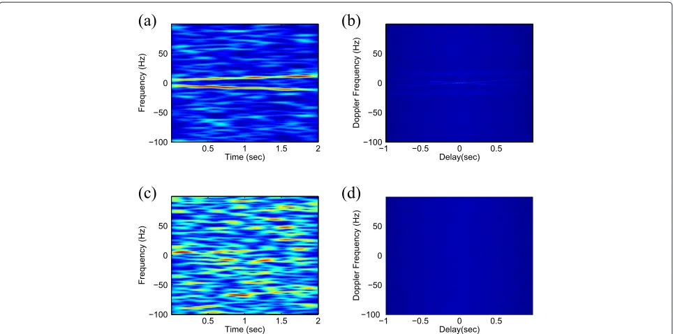
The spectrogram and the ambiguity function of Doppler signatures of two targets corresponding to the first illu-minator are presented in Figure 2 at two different SNR conditions. For high SNR applications, as illustrated in Figure 2a,b, the spectrogram constitutes two distinct lines corresponding to the respective initial frequency and chirp rate of the Doppler signatures of the two targets. The ambiguity function, on the other hand, constitutes two distinct straight lines passing through the origin, with different slopes depending on the respective chirp rates. As such, the chirp parameters can be reliably estimated for each bistatic link using time-frequency analysis-based methods, and subsequently, the respective motion param-eters can be estimated using (11) by using the standard least squares (LS) methods. However, when the input SNR is low, as evident in Figure 2c,d, it is difficult to reliably obtain chirp parameters corresponding to each bistatic link. The chirp parameter estimation process in the pres-ence of additive white Gaussian noise suffers a rapid performance degradation below a certain SNR threshold. This necessitates a mechanism to combine signal energy from all available bistatic links which, however, is diffi-cult to implement directly in the time-frequency domain. By exploiting sparsity-based signal reconstruction, the ML and the two-step sequential methods, respectively, pro-vide a means to coherently and non-coherently combine Doppler signatures from all available links. They result in an overall signal enhancement, and consequently, the threshold is reached at a lower SNR as compared to the traditional time-frequency analysis-based methods.
The performance of the sparse signal reconstruction-based methods is compared against the CRB formulated in (34) for the underlying problem. For the given sim-ulation scenario, we obtain the root-mean-square error (RMSE) of the estimated acceleration and velocity through 100 independent trials, and the results are, respectively, presented in Figure 3a,b.
Time (sec)
Frequency (Hz)
0.5 1 1.5 2
−100 −50 0 50
(a)
Doppler Frequency (Hz)
Delay(sec)
−1 −0.5 0 0.5
−100 −50 0 50
(b)
Time (sec)
Frequency (Hz)
0.5 1 1.5 2
−100 −50 0 50
(c)
Doppler Frequency (Hz)
Delay(sec)
−1 −0.5 0 0.5
−100 −50 0 50
(d)
Figure 2Spectrogram and ambiguity function of Doppler signature for two targets at high and low SNR.(a)Spectrogram (SNR= −45 dB).
(b)Ambiguity function (SNR= −45 dB).(c)Spectrogram (SNR= −53 dB).(d)Ambiguity function (SNR= −53 dB).
proposed method. As discussed in Section 3, representa-tion of target morepresenta-tion parameters in a discretized param-eter space may yield an off-grid problem. However, in the simulated example, we have defined the grid resolution fine enough to match the CRB, such that the performance is robust even if the true parameter is off-grid. Specif-ically, grid resolutions used in this simulated example are 0.05 m/s2 for acceleration and 0.01 m/s for velocity estimation, respectively.
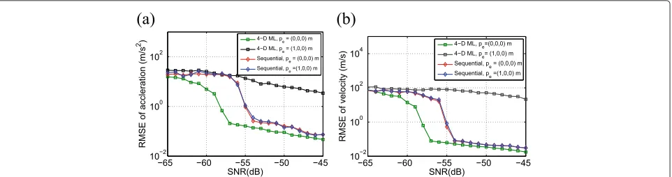
As discussed in Section 4, errors in the assumed or estimated initial positions of the targets result in phase differences among the Doppler signatures corresponding to different bistatic links. In such a situation, depending upon the phase interactions, the individual Doppler natures may destructively add to each other, yielding a sig-nificant reduction in overall signal energy accumulation
through a coherent fusion process. As such, the ML search-based motion parameter estimation suffers a per-formance degradation in case of an imperfect knowledge about the initial positions of the targets. On the other hand, the sequential method does not rely on coherent combining of the Doppler signatures for overall signal enhancement and, hence, is robust against such phase misalignment. In order to illustrate such situation, we consider a position error of [1, 0, 0]T m, which is approx-imately equal to the wavelength of operation, in the esti-mation of the initial positions of both targets. It is evident in Figure 5 that the ML search-based motion parameter error suffers a significant performance loss, whereas the two-step sequential method is robust against such local-ization error, which is an observation of high practical significance.
−65 −60 −55 −50 −45
10−2 10−1 100 101 102
RMSE of accleration (m/s
2)
SNR(dB)
CRB 4−D ML Chirp Tran. Sequential
(a)
−65 −60 −55 −50 −45
10−2 10−1 100 101 102
RMSE of velocity (m/s)
SNR(dB)
CRB 4−D ML Chirp Tran. Sequential
(b)
−65 −60 −55 −50 −45 10−2
10−1 100 101 102
RMSE of accleration (m/s
2)
SNR(dB)
7 Tx 5 Tx
(a)
−65 −60 −55 −50 −45
10−2 10−1 100 101 102
RMSE of velocity (m/s)
SNR(dB)
7 Tx 5 Tx
(b)
Figure 4Comparison of RMSE of parameter estimation using different numbers of transmitters.(a)Acceleration.(b)Velocity.
It is important to note that there are two sources of error that are inherently associated with the target accel-eration estimation using the proposed method. Since the ambiguity function, defined in (18), is bilinear, the effect of noise is enhanced, resulting in a performance degra-dation as compared to its linear transform counterpart. Furthermore, since matrix mapping the chirp parameters to the respective motion parameters, defined in (12), is not exactly block diagonal, the target velocity does have a small effect on the chirp rate. This introduces an estima-tion error in the acceleraestima-tion because target velocity is not considered in (19). The significance of the error is propor-tional to the ratio of velocity of the receiver platform to the target-receiver separation. That is, the effect of this off-diagonal block becomes insignificant for distant targets. In the simulated example, the off-diagonal term is small, yielding negligible acceleration estimation error. Specif-ically, in the simulated example, the off-diagonal term is approximately [0.015, 0, 0]T 1/s and the corresponding
acceleration estimation error is approximately 0.004 m/s2.
Velocity estimation, on the other hand, involves a linear process. Therefore, it does not suffer from performance degradation due to bilinear effects as in acceleration estimation. However, the error which occurred in the estimated target acceleration propagates to the velocity
estimation, and the significance of such error propagation depends on the duration of the CPI. Also, when the target motion parameters are closely located in the parameter space, the performance deteriorates specially in low SNR conditions.
6 Conclusions
We have developed novel methods for the estimation of motion parameters of multiple closely located ground moving targets in a multi-static passive radar plat-form. By exploiting the fact that the Doppler signatures of the targets corresponding to different bistatic links share the same target motion parameters as a com-mon sparse support in the discretized parameter search space, the underlying problem is reformulated as a group sparse signal reconstruction problem. The sparse signal reconstruction-based methods allow for the fusion of data from all bistatic links, which is not possible in tradi-tional time-frequency analysis-based methods. The two-step sequential method emphasizes on decoupling the effects of target acceleration and velocity on the Doppler signature and obtains a sequential estimation of the target motion parameters to avoid the need for a computation-ally demanding multi-dimensional exhaustive search. It is shown that the sequential method also outperforms
−65 −60 −55 −50 −45
10−2 100 102
RMSE of accleration (m/s
2)
SNR(dB)
4−D ML, pe = (0,0,0) m 4−D ML, pe = (1,0,0) m Sequential, pe = (0,0,0) m Sequential, pe =(1,0,0) m
(a)
−65 −60 −55 −50 −45
10−2 100 102 104
RMSE of velocity (m/s)
SNR(dB)
4−D ML, pe=(0,0,0) m 4−D ML, pe= (1,0,0) m
Sequential, pe = (0,0,0) m
Sequential, pe =(1,0,0) m
(b)
Figure 5Comparison of RMSE of parameter estimation considering an imperfect knowledge of initial target positions.(a)Acceleration.
the maximum likelihood search-based parameter esti-mation in cases where the initial positions of the tar-gets is not precisely known. The performance of the proposed estimators is validated by simulations, and it is shown that these approaches outperform the time-frequency analysis-based methods and closely approaches the Cramér-Rao Bound.
Competing interests
The authors declare that they have no competing interests.
Acknowledgements
The work of S. Subedi, Y. D. Zhang, and M. G. Amin was supported in part by a subcontract with Defense Engineering Corporation for research sponsored by the Air Force Research Laboratory under Contract FA8650-12-D-1376 and by a subcontract with Dynetics, Inc. for research sponsored by the Air Force Research Laboratory under Contract FA8650-08-D-1303. Part of the work was presented in the 2014 IEEE International Conference on Acoustics, Speech, and Signal Processing [35].
Author details
1Center for Advanced Communications, Villanova University, Villanova, PA
19085, USA.2RF Technology Branch, Air Force Research Laboratory,
AFRL/RYMD, Dayton, OH 45433, USA.
Received: 28 June 2014 Accepted: 9 October 2014 Published: 24 October 2014
References
1. H Griffitths, N Long, Television-based bistatic radar. IEE Proc. Commun. Radar Signal Proc.133(7), 649–657 (1986)
2. S Subedi, YD Zhang, MG Amin, B Himed, inProceedings of European Signal Processing Conference. Robust motion parameter estimation in multistatic passive radar (Marrakech, Morocco, Sept. 2013)
3. GR Curry,Radar System Performance Modeling, 2nd ed, (Artech House, Norwood, 2005)
4. MI Skolnik,Introduction to Radar Systems, 3rd ed, (McGraw-Hill, New York, 2001)
5. A Hassanien, SA Vorobyov, AB Gershman, Moving target parameter estimation in noncoherent MIMO radar systems. IEEE Trans. Signal Process.60(5), 2354–2361 (2012)
6. Q He, RS Blum, H Godrich, AM Haimovich, inProceedings of Annual Conference on Information Sciences and Systems. Cramer-Rao bound for target velocity estimation in MIMO radar with widely separated antennas (Princeton, NJ, Mar. 2008)
7. Q He, RS Blum, AM Haimovich, Noncoherent MIMO radar for location and velocity estimation: more antennas means better performance. IEEE Trans. Signal Process.58(7), 3661–3680 (2010)
8. Y Zhang, MG Amin, F Ahmad, inProceedings of Asilomar Conference on Signals, Systems, and Computers. A novel approach for moving multi-target localization using dual frequency radars and time-frequency distributions (Pacific Grove, CA, Nov. 2007), pp. 1817–1821
9. F Zhou, R Wu, M Xing, Z Bao, Approach for single channel SAR ground moving target imaging and motion parameter estimation. IET Radar, Sonar Navigation.1(1), 59–66 (2007)
10. SQ Zhu, GS Liao, Y Qu, ZG Zhou, inProceedings of IEEE Radar Conference. Ground moving targets detection and unambiguous motion parameter estimation based on multi-channel SAR system, (April 2009), pp. 1–4 11. M Kubica, V Kubica, X Neyt, J Raout, S Roques, M Acheroy, inProceedings
of IEEE Radar Conference. Optimum target detection using illuminators of opportunity, (April 2006), pp. 24–27
12. AP Whitewood, BR Muller, HD Griffiths, CJ Baker, inProceedings of IEEE Radar Conference. Bistatic synthetic aperture radar with application to moving target detection, (Sept. 2003), pp. 529–534
13. A Scaglione, S Barbarossa, inProceedings of IEEE Radar Conference. Estimating motion parameters using parametric modeling based on time-frequency representations (Syracuse, NY, Oct. 1997)
14. S Stankovi, I Djurovi, Motion parameter estimation by using time-frequency representations. IEEE Electron. Lett.37(24), 1446–1448 (2001)
15. YD Zhang, B Himed, inProceedings of IEEE Radar Conference. Moving target parameter estimation and SFN ghost rejection in multistatic passive radar (Ottawa, Canada, April 2013)
16. S Peleg, B Porat, The Cramer-Rao lower bound for signals with constant amplitude and polynomial phase. IEEE Trans. Signal Process.39(3), 749–752 (1991)
17. S Saha, SM Kay, Maximum likelihood parameter estimation of
superimposed chirps using Monte Carlo importance sampling. IEEE Trans. Signal Process.50(2), 224–230 (2002)
18. C Berger, B Demissie, J Heckenbach, P Willett, S Zhou, Signal processing for passive radar using OFDM waveforms. IEEE J. Selected Topics Signal Process.4(1), 226–238 (2010)
19. RP Perry, RC DiPietro, R Fante, inProceedings IEEE Radar Conference. Coherent integration with range migration using Keystone formatting (Boston, MA, April 2007), pp. 863–868
20. B Boashash,Time Frequency Signal Analysis and Processing: A Comprehensive Reference. (Elsevier, Oxford, UK, 2003)
21. GC Gaunaurd, HC Strifors, Signal analysis by means of time-frequency (Wigner-type) distributions-applications to sonar and radar echoes. Proc. IEEE.84(9), 1231–1248 (1996)
22. V Chen, H Ling, Joint time-frequency analysis for radar signal and image processing. IEEE Signal Process. Mag.16(2), 81–93 (1999)
23. HB Sun, G-S Liu, H Gu, W-M Su, Application of the fractional Fourier transform to moving target detection in airborne SAR. IEEE Trans. Aero. Electron. Syst.38(4), 1416–1424 (2002)
24. S Barbarossa, Analysis of multicomponent LFM signals by a combined Wigner-Hough transform. IEEE Trans. Signal Process.43(6), 1511–1515 (1995)
25. EVD Berg, M Friedlander, Probing the Pareto frontier for basis pursuit solutions. SIAM J. Sci. Comput.31(2), 890–912 (2008)
26. M Yuan, Y Lin, Model selection and estimation in regression with grouped variables. J. Roy. Stat. Soc. B.68(1), 49–67 (2006)
27. L Zelnik-Manor, K Rosenblum, YC Eldar, Sensing matrix optimization for block-sparse decoding. IEEE Trans. Signal Process.59(9), 4300–4312 (2011) 28. S Ji, D Dunson, L Carin, Multitask compressive sensing. IEEE Trans. Signal
Process.57(1), 92–106 (2009)
29. Q Wu, YD Zhang, MG Amin, B Himed, inProceedings of IEEE International Conference on Acoustics, Speech, and Signal Processing (ICASSP). Complex multi-task Bayesian compressive sensing (Florence, Italy, May 2014) 30. M Carlin, P Rocca, G Oliveri, F Viani, A Massa, Directions-of-arrival
estimation through Bayesian compressive sensing strategies. IEEE Trans. Antenn. Propag.61(7), 3828–3838 (2013)
31. S Kay,Fundamentals of Statistical Signal Processing: Estimation Theory. (Prentice-Hall, Englewood Cliffs, 1993)
32. C Coleman, H Yardley, inProceedings of International Conference on Radar. DAB based passive radar: performance calculations and trials (Adelaide, Australia, Sept. 2008), pp. 691–694
33. B Friedlander, JM Francos, Estimation of amplitude and phase parameters of multicomponent signals. IEEE Trans. Signal Process.43(4), 917–925 (1995)
34. S Peleg, B Friedlander, inProceedings of IEEE-SP International Symposium of the Time-Frequency and Time-Scale Analysis. A technique for estimating the parameters of multiple polynomial phase signals (Victoria, Canada, Oct. 1992)
35. S Subedi, YD Zhang, MG Amin, B Himed, inProceedings of IEEE International Conference on Acoustics, Speech, and Signal Processing (ICASSP). Motion parameter estimation of multiple targets in multistatic radar through sparse signal recovery (Florence, Italy, May 2014)
doi:10.1186/1687-6180-2014-157