A regularized matrix factorization approach to induce structured sparse low rank solutions in the EEG inverse problem

R E S E A R C H

Open Access

A regularized matrix factorization approach to

induce structured sparse-low-rank solutions in

the EEG inverse problem

Jair Montoya-Martínez

, Antonio Artés-Rodríguez

, Massimiliano Pontil

and Lars Kai Hansen

Abstract

We consider the estimation of the Brain Electrical Sources (BES) matrix from noisy electroencephalographic (EEG) measurements, commonly named as the EEG inverse problem. We propose a new method to induce

neurophysiological meaningful solutions, which takes into account the smoothness, structured sparsity, and low rank of the BES matrix. The method is based on the factorization of the BES matrix as a product of a sparse coding matrix and a dense latent source matrix. The structured sparse-low-rank structure is enforced by minimizing a regularized functional that includes the21-norm of the coding matrix and the squared Frobenius norm of the latent source matrix. We develop an alternating optimization algorithm to solve the resulting nonsmooth-nonconvex minimization problem. We analyze the convergence of the optimization procedure, and we compare, under different synthetic scenarios, the performance of our method with respect to the Group Lasso and Trace Norm regularizers when they are applied directly to the target matrix.

Keywords: Structured sparsity; Low rank; Matrix factorization; Regularization; Nonsmooth-nonconvex optimization

1 Introduction

The solution of the electroencephalographic (EEG) inverse problem to obtain functional brain images is of high value for neurological research and medical diag-nosis. It involves the estimation of the Brain Electrical Sources (BES) distribution from noisy EEG measure-ments, whose relation is modeled according to the linear model

Y=AS+E, (1)

whereY ∈ RM×T andA ∈ RM×N are known and

rep-resent, respectively, the EEG measurements matrix and the forward operator (a.k.a lead field matrix),S∈ RN×T denotes the BES matrix, andE∈RM×T is a noise matrix.

Mdenotes the number of EEG electrodes,Nis the num-ber of brain electrical sources, andTis the number of time instants.

*Correspondence: [email protected]

1Department of Signal Processing and Communications, Universidad Carlos III de Madrid, Avda. Universidad 30, Leganés, Madrid 28911, Spain

Full list of author information is available at the end of the article

This estimation problem is very challenging:N M, and the existence of silent BES (BES that produce non-measurable fields on the scalp surface) implies that the EEG inverse problem has infinite solutions: a silent BES can always be added to a solution of the inverse problem without affecting the EEG measurements. For all these reasons, the EEG inverse problem is an undetermined ill-posed problem [1-4].

A classical approach to solve an ill-posed problem is to use regularization theory, which involves the replacement of the original ill-posed problem with a ‘nearby’ well-posed problem whose solution approximates the required solution [5]. Solutions developed by this theory are stated in terms of a regularization function, which helps us to select, among the infinite solutions, the one that best fulfills a prescribed constrain (e.g., smoothness, spar-sity, and low rank). To define the constrain, we can use mathematical restrictions (minimum norm estimates) or anatomical, physiological, and functional prior informa-tion. Some examples of useful neurophysiological infor-mation are [1,6]: the irrotational character of the brain current sources, the (smooth) dynamic of the neural sig-nals, the clusters formed by neighboring or functional

related BES, and the smoothness and focality of the elec-tromagnetic fields generated and propagated within the volume conductor media (brain cortex, skull, and scalp).

Several regularization functions have been proposed in the EEG community: Hämäläinen and Ilmoniemi in [7] proposed a squared Frobenius norm penalty (S2

F), which they named Minimum Norm Estimate (MNE). This reg-ularization function usually induces solutions that spread over a considerable part of the brain. Uutela et al. in [8] proposed an 1-norm penalty (S1). They named their approach Minimum Current Estimate (MCE). This penalty function promotes solutions that tend to be scat-tered around the true sources. Mixed12-norm penal-ties have also been proposed in the framework of the time basis, time frequency dictionaries, and spatial basis decomposition. These mixed norm approaches induce structured sparse solutions and depend on decomposing the BES signals as linear combinations of multiple basis functions, e.g., Ou et al. in [9] proposed the use of tem-poral basis functions obtained with singular value decom-position (SVD), Gramfort et al. in [10,11] proposed the use of time-frequency Gabor dictionaries, and Haufe et al. in [12] proposed the use of spatial basis Gaussian func-tions. For a more detailed overview on inverse methods for EEG, see [2,3,13] and references therein. For a more detailed overview on regularization functions applied to structured sparsity problems, see [14-16] and references therein.

All of these regularizers try to induce neurophysiolog-ical meaningful solutions, which take into account the smoothness and structured sparsity of the BES matrix: during a particular cognitive task, only the BES related with the brain area involved in such a task will be active, and their corresponding time evolution will vary smoothly, that is, the BES matrix will have few nonzero rows, and in addition, the columns will vary smoothly. In this paper, we propose a regularizer that takes into account not only the smoothness and structured sparsity of the BES matrix but also its low rank, capturing this way the linear relation between the active sources and their corresponding neighbors. In order to do so, we propose a new method based on matrix factorization and regulariza-tion, with the aim of recovering the latent structure of the BES matrix. In the factorization, the first matrix, which acts as a coding matrix, is penalized using the21-norm, and the second one, which acts as a dense, full rank latent source matrix, is penalized using the squared Frobenius norm.

In our approach, the resulting optimization problem is nonsmooth and nonconvex. A standard approach to deal with the nonsmoothness introduced by the nons-mooth regularizers mentioned above is to reformulate the regularization problem as a second-order cone program-ming (SOCP) problem [12] and use interior point-based

solvers. However, interior point-based methods can not handle large scale problems, which is the case of large EEG inverse problems involving thousands of brain sources. Another approach is to try to solve the nonsmooth problem directly, using general nonsmooth optimization methods, for instance, the subgradient method [17]. This method can be used if a subgradient of the objective function can be computed efficiently [14]. However, its convergence rate is, in practice, slow (O(1/√k)), wherek

is the iteration counter. In this paper, in order to tackle the nonsmoothness of the optimization problem, we depart from these optimization methods and use instead efficient first-order nonsmooth optimization methods [5,18,19]: forward-backward splitting methods. These methods are also called proximal splitting because the nonsmooth function is involved via its proximity operator. Forward-backward splitting methods were first introduced in the EEG inverse problem by Gramfort et al. [10,11,13], where they used them to solve nonsmooth optimization prob-lems resulting from the use of mixed12-norm penalties functions. These methods have drawn, increasing atten-tion in the EEG, machine learning, and signal processing community, especially because of their convergence rates and their ability to deal with large problems [19-21].

On the other hand, in order to handle the nonconvexity of the optimization problem, we use an iterative alternat-ing minimization approach: minimizalternat-ing over the codalternat-ing matrix while maintaining fixed the latent source matrix and viceversa. Both of these optimization problems are convex: the first one can be solved using proximal split-ting methods, while the second one can be solve directly in terms of a matrix inversion.

The rest of the paper is organized as follows. In Section 2, we give an overview of the EEG inverse prob-lem. In Section 3, we present the mathematical back-ground related with the proximal splitting methods. The resulting nonsmooth and nonconvex optimization prob-lem is formally described in Section 4. In Section 5, we propose an alternating minimization algorithm, and its convergence analysis is presented in Section 6. Section 7 is devoted to the numerical evaluation of the algorithm and its comparison with the Group Lasso and Trace Norm regularizers, which consider partially the characteristics of the matrix S: its structured sparsity by using the21 -norm and its low rank by using the∗-norm, respectively. The advantages of considering both characteristics in a single method, like in the proposed one, become clear in comparison with the independent use of the Group Lasso and Trace Norm regularizers. Finally, conclusions are presented in Section 8.

2 EEG inverse problem background

assembly is small compared to the distance to the obser-vation point (the EEG sensors). Therefore, the electro-magnetic fields produced by an active neuron assembly at the sensor level are very similar to the field pro-duced by a current dipole [23]. This simplified model is known as the equivalent current dipole (ECD). These ECDs are also known by other names such as BES and current sources. Due to the uniform spatial orga-nization of their dendrites (perpendicular to the brain cortex), the pyramidal neurons are the only neurons that can generate a net current dipole over a piece of cortical surface, whose field is detectable on the scalp [3]. According to [24], it is necessary to add the field of∼ 104pyramidal neurons in order to produce a volt-age that is detectable on the scalp. These voltvolt-ages can be recorded by using different types of electrodes [22], such as disposable (gel-less, and pre-gelled types), reusable disc electrodes (gold, silver, stainless steel, or tin), headbands and electrode caps, saline-based electrodes, and needle electrodes.

Under the quasi-static approximation of Maxwell’s equations, we can express the general model for the observed EEG signalsy(t)at timetas linear functions of the BESs(t)[9]:

y(t)=As(t)+e(t), (2)

where y(t) ∈ RM×1 is the EEG measurements

vec-tor, s(t) ∈ RN×1 is the BES vector, e(t) ∈ RM×1

is the noise vector, and A ∈ RM×N is the lead field matrix. In a typical experimental setup, the number of electrodes (M) is ∼ 102_{, and the number of BES (N)}

is ∼ 103_{, 10}4_{. We can express the former model}

for all time instants {t1,t2,. . .,tT} (corresponding to some observation time window) by using the matrix formulation (1), where Y = y(t1),y(t2),. . .,y(tT)

∈ RM×T_{, S = [s(t}

1),s(t2),. . .,s(tT)] ∈ RN×T, and E = [e(t1),e(t2),. . .,e(tT)]∈RM×T. Theith row of the matrix Y represents the electrical activity recorded by the ith EEG electrode during the observation time window. In the BES matrixS, each row represents the time evolution of one brain electrical source, and each column repre-sents the activity of all the corresponding sources in a particular time instant. Finally, the forward operator A summarizes the geometric and electric properties of the conducting media (brain, skull, and scalp) and establishes the link between the current sources and EEG sensors (Aij tells us how thejth BES influences the measure obtained by the ith electrode). Following this notation, the EEG inverse problem can be stated as follows: Given a set of EEG signals (Y) and a forward model (A), estimate the current sources within the brain (S) that produce these signals.

3 Mathematical background

3.1 Proximity operator

The proximity operator [19,25] corresponding to a convex functionf is a mapping fromRnto itself and is defined as follows:

prox_f(z)=argmin x∈Rn

f(x)+1

2x−z 2

, (3)

where · denotes the Euclidean norm. Note that the

proximity operator is well defined, because the above minimum exists and is unique (the objective function if strongly convex).

3.2 Subdifferential-proximity operator relationship Iff is a convex function onRnandy∈Rn, then [26]

x∈∂f(y)⇔y=prox_f(x+y), (4) where∂f(y)denotes the subdifferential off aty.

3.3 Principles of proximal splitting methods

Proximal splitting methods are specifically tailored to solve an optimization problem of the form

minimize

S f(S)+r(S), (5)

wheref(S)is a smooth convex function, andr(S)is also a convex function, but nonsmooth. From convex analysis [17], we know thatSis a minimizer of (5) if and only if 0∈∂(f +r)(S). This implies the following [18]:

0∈∂(f +r)(S) ⇔ 0∈ {∂f(S)+∂r(S)}

⇔ −∇f(S)∈∂r(S)

⇔ −γ∇f(S)∈γ ∂r(S)

⇔ (S−γ∇f(S))−S∈∂γr(S)

Using (4) in the former expression, we get

S=prox_γr(S−γ∇f(S)) (6)

Equation 6 suggests that we can solve (5) using a fixed point iteration:

S_k+1=prox_γr(Sk−γ∇f(Sk)) (7) In optimization, (7) is known as forward-backward split-ting process [19]. It consists of two steps: first, it performs a forward gradient descend stepS∗_k = Sk−γ∇f(Sk)and then it performs a backward stepS_k+1=proxγr(S∗k).

For instance, the Iterative Soft Thresholding Algorithm (ISTA) has a convergence rate of O(1/k), and the Fast

Iterative Shrinkage-Thresholding Algorithm (FISTA) has a convergence rate ofO(1/k2)[5].

4 Problem formulation

The regularized EEG inverse problem can be stated as follows: denotes the Frobenius norm), andλ(S)is a nonsmooth penalty term that is used to encode the prior knowledge about the structure of the target matrixS.

In order to induce structured sparse-low-rank solutions, we propose to reformulate (1) using a matrix factorization approach, which involves expressing the matrixSas the product of two matrices,S=BC, obtaining the following nonlinear estimation model:

Y=ABC+E, (9)

where B and C are penalized using the 21-norm and

the squared Frobenius norm, respectively. The resulting optimization problem can be stated as follows:

ˆ

In this formulation, which we denote as matrix factor-ization approach, the21-norm and the squared Frobenius norm induce structured sparsity and smoothness in the rows ofB andC, respectively, and therefore also in the rows ofS. Finally, the parameterKencloses the low rank ofS:

rank(B)≤ min{N,K} ⇒rank(B)≤ K

rank(C)≤ min{K,T} ⇒rank(C)≤ K

rank(BC)≤ min{rank(B), rank(C)} ≤K

⇒rank(S)≤ K

Hence, the proposed regularization framework takes into account all the prior knowledge about the structure of the target matrixS.

5 Optimization algorithm

5.1 Matrix factorization approach

In this section, we address the issue of implementing the learning method (10) numerically. We propose the following reparameterization of (10):

B=λρB˜, C= √1

Using (11) in the objective function of (10), we get

⇒ 1 problem with only one regularization parameter:

ˆ

The optimization problem (12) is a simultaneous mini-mization over matricesBandC. For a fixedC, the mini-mum overBcan be obtained using FISTA. On the other hand, for a fixed B, the minimum overC can be solved directly in terms of a matrix inversion. These observations suggest an alternating minimization algorithm [15,28]:

Algorithm 1Alternating minimization algorithm to solve the matrix factorization-regularization-based approach

Require: Y∈RM×T_,A∈RM×N_,C

untilstopping condition is met

Y. Without loss of generality, let us work with (9) in the noiseless case:

Y=ABC (15)

From (15), we can see that {Y1,Y2,. . .,YM} ⊂ Row Space(C), whereYidenotes theith row ofY.

Now, let us obtain a rank-Kapproximation ofYby using a truncated SVD (truncated at the singular valueσK):

Y≈UM×K K×KVK×T (16)

From the SVD theory [29], we know that

{Y1,Y2,. . .,YM} ⊂ Row SpaceV; therefore, we can chooseC0 = V. Then, givenC0, we can start iterating using (13) and (14).

5.1.1 Minimization overB(fixedC)

The minimization overBcan be stated as follows:

Bt=argmin B

FB(B)+λB2,1,λ >0

, (17)

whereFB(B) = 1₂A(BCt−1)−Y2_F+ 1₂Ct−12_F. This is a composite convex optimization problem involving the sum of a smooth function (FB(B)) and a nonsmooth

func-tion (λB2,1). As we have seen in Section 3, this kind of problem can be efficiently handled using proximal split-ting methods (e.g., FISTA). In order to apply FISTA to solve (17), we first need to compute the following:

1. The gradient of the smooth functionFB(B)

∇FB(B)= ∂FB(B)

∂B =A(A(BCt−1)−Y)Ct−1

whereAdenotes the transpose of the matrixA. 2. An upper bound of the Lipschitz constant (L) of

∇FB(B)(it can also be estimated using a backtracking search routine [5])

∇FB(B1)−∇FB(B2)22=AAB1Ct−1Ct−1

−AAB2Ct−1Ct−122

=AA(B1−B2)Ct−1Ct−122

= K

j=1

A_A(B

1−B2) Ct−1Ct−1

j

2 2

whereCt−1C_t−1jdenotes thej-th column of the

matrixCt−1C_t−1. Taking into account that Qx2≤ |Q|2x2, ∀x∈RN,∀Q∈RM×N[29],

where| · |2denotes the spectral norm , we get:

∇FB(B1)− ∇FB(B2)22= K

j=1

AA(B1−B2)

×Ct−1Ct−1

j 2 2

≤ K

j=1

|A_A(B

1−B2)|22

× C_t−1C t−1

j 2 2

≤ |AA(B1−B2)|22

× K

j=1

Ct−1Ct−1

j 2 2

≤ |A_A(B

1−B2)|22 × C_t−1Ct−122

(18)

From (18), taking into account that the spectral norm is submultiplicative (|PQ|2≤ |P|2|Q|2, ∀P∈ RM×N_{, ∀Q∈R}N×T_{), it follows that:}

∇FB(B1) − ∇FB(B2)22≤ |AA|22 |B1 − B2|22|Ct−1Ct−122

and, using the fact that|P|2₂≤ P2₂, ∀P∈RM×N, we obtain:

∇FB(B1)− ∇FB(B2)22≤ |AA|22B1−B222 × Ct−1Ct−122

≤LB1−B222 (19)

whereL= |AA|2Ct−1C_t−12.

3. Proximal operator associated to the nonsmooth functionλ· 2,1

prox_λ·2,1(B)=argmin X

λX2,1+ 1

2X−B 2 2

=prox_λ·2,1(B)

i,: i=N

i=1 =

_B i,: Bi,:2(

Bi,:2−λ)+ i=N

i=1

(20)

where(·)+=max(·, 0), and by convention0₀=0.

5.1.2 Minimization overC(fixedB)

The minimization overCcan be stated as follows:

Ct=argmin

C {FC(C)} (21)

the minimum overCcan be solved directly in terms of a matrix inversion:

∇FC(C)= ∂FC(C)

∂C =BtA(A(BtC)−Y)+C

∇FC(C)=0⇒BtA(A(BtCt)−Y)+Ct=0 ⇒Ct=

BtAABt+IK −1

BtAY

(22)

The matrixBtAABt+IK

∈ RK×K_{, andK is} sup-posed to be small; therefore, calculating its corresponding inverse matrix is quite cheap.

6 Convergence analysis

We are going to analyze the convergence behavior of Algorithm 1 by using the global convergence theory of iterative algorithms developed by Zangwill [30]. Note that in this theory, the term ‘global convergence’ do not imply convergence to a global optimum for all initial points. The property of global convergence expresses, in a sense, the certainty that the algorithm converges to the solution set. Formally, an iterative algorithm ξ, on the set X, is said to be globally convergent provided, for any starting point

x0∈X, the sequence{xn}generated byξhas a limit point [31].

In order to use the global convergence theory of iterative algorithms, we need a formal definition of iterative algo-rithm, as well as the definition of a set-valued mapping (a.k.a point-to-set mapping) [30]:

Definition 6.1. Set-valued mapping. Given two sets, X

and Y , a set-valued mapping defined on X, with range in the power set of Y ,P(Y), is a map,, which assigns to each x∈X a subset(x)∈P(Y),

:X→P(Y)

Definition 6.2. Iterative algorithm. Let X be a set and x0 ∈X a given point. Then, an iterative algorithmξ, with initial point x0, is a set-valued mapping

ξ:X→P(X)

which generates a sequence {xn}∞_n=1 via the rule xn+1 ∈ ξ(xn), n=0, 1,. . .

Now that we know the main building blocks of the global convergence theory of iterative algorithms, we are in a position to state the convergence theorem related to Algorithm 1:

Theorem 6.1. Letdenotes the iterative Algorithm 1, and suppose that givenY ∈ RM×T,A∈ RM×N,B0 ∈ RN×K,

C0∈RK×T, K , andλ, the sequence{Bt,Ct}∞_t=1is generated and satisfies {Bt+1,Ct+1} ∈ (Bt,Ct). Also, letBand

Cdenote the solution sets of (13)and(14), respectively:

B=

B∈RN×K_0∈∂

1

2||A(BCt−1)−Y|| 2

F+λ||B||2,1

+ 1

2||Ct−1|| 2

F

C=

C∈RK×T_∇

1

2||A(BtC)−Y|| 2

F+λ||Bt||2,11 2||C||

2

F

=0

Then, the limit of any convergent subsequence of

{Bt,Ct}∞_t=1is inBandC.

This convergence theorem is a direct application of Zangwill’s global convergence theorem [30]. Before going in this assertion, let us show some definitions and theo-rems used in the proof.

Definition 6.3. Compact set. A set X is said to be com-pact if any sequence (or subsequence) contains a convergent subsequence whose limit is in X. More explicitly, given a subsequence{xn}_n∈Nin X, there exists aN1⊂N such that

xn→x∞, n∈N1

with x∞ ∈ X (we write convergence of subsequences as xn→x∞, which is equivalent to_n→∞limxn=x∞).

Definition 6.4. Composite map. LetA : X → Y and

B :Y →Z be two set-valued mappings. The composite map C = B◦A which takes points x ∈ X to sets

C(x)⊂Z is defined by

C(x):=

y∈A(x)

B(y)

Definition 6.5. Closed map. A set-valued mapping :

X→P(Y)is closed at x0∈X provided

1. xn→x0as n→ ∞, xn∈X

2. yn→y0as n→ ∞, yn, y0∈Y

3. yn∈(xn)

implies y0 ∈(x0). The mapis called closed on S⊂X provided is closed at each x∈S.

Theorem 6.2. Composition of closed maps. LetA:X→

Y andB:Y →Z be two set-valued mappings. Suppose

1. Ais closed atx0

2. Bis closed onA(x0)

3. ifxn→x0andyn∈A(xn), then there exists

y0∈Y, such that for some sequence

ynj

,ynj →y0

asj→ ∞.

Then, the composite mapC =B◦Ais closed at x0.

Lemma 6.1. [32] Given a real-valued function defined on X×Y , define the set-valued mapping:X→P(Y)by

(x)=argmin y∈Y h(x,y)

Theorem 6.3. Weierstrass theorem. If f is a real

con-Theorem 6.4. [30] Zangwill’s global convergence theorem. Let the set-valued mapping Mx(x):X→P(X)determine an algorithm that given a point x0 generates a sequence {xn}∞_n=0 through the iteration xn+1 ∈ Mx(xn). Also, let a solution setbe given. Suppose

1. All pointxnare in a compact setS⊂X.

2. There is a continuous functionα:X→Rsuch that

(a) ifx∈/, thenα(x) < α(x)∀x∈Mx(x). (b) ifx∈, thenα(x)≤α(x)∀x∈Mx(x). 3. The mapMx(x)is closed atxifx∈/.

Then, the limit of any convergent subsequence of{xn}∞_n=0 is in. That is, accumulation points x∗of the sequence xn

lie in. Furthermore,α(xn)converges toα∗, andα(x∗)=α∗ for all accumulation points x∗.

Proof.Theorem 6.1. The iterative algorithm can be decomposed into two well-defined iterative algorithms BandC:

As we can see from (23) and (24), at iterationt, the result ofB becomes the input of C, and at iteration t+1, the result ofC becomes the input ofB; therefore, we can expressas the composition ofC andB, that is, (Ct−1)= C(B(Ct−1)): To prove this theorem by using Zangwill’s global conver-gence theorem, we need to prove that all its corresponding assumptions are fulfilled. In order to prove assumption 1, let us analyze the sequences{Bt}∞_t=1 and{Ct}∞_t=1. The sequence {Bt}∞_t=1 is generated by using FISTA, which is a convergent algorithm (Bt → B∞) that guarantees that

Bt ∈ B [5,18]. Hence, using Definition 6.3, we can

see that the sequence{Bt}∞_t=1generated by (23) lies in a compact set. On the other hand, the sequence{Ct}∞_t=1is generated by (22), which guarantees thatCt ∈ C. This sequence always converges to a point inside C, which implies thatC also lies in a compact set. This concludes the proof of assumption 1.

To prove assumption 2, let us useZ(C,t)as the function α(·); thus, in order to verify the fulfillment of assumption 2, we need to prove that

(a) ifCt∈/, thenZ(Ct+1,t+1) <Z(Ct,t)∀Ct+1∈ (Ct)

(b) ifCt∈, thenZ(Ct+1,t+1)≤Z(Ct,t)∀Ct+1∈ (Ct)

From (25), we can see that the sequence {Ct}∞_t=1 will always lie in(becauseCtis generated by (22)); therefore, we only need to prove (b).

1

and from (26) and (27), we can prove assumption 2(b):

1

In order to prove assumption 3, we need to prove that is closed atCifC ∈/ . To do so, we are going to use Theorem 6.2; therefore, we need to prove thatBandC are both closed maps: from (23) and (24), we can see that their corresponding objective functions are both continu-ous∀B∈RN×K and∀C∈ RK×T, respectively; hence, by using Weierstrass Theorem and Lemma 6.1, we can con-clude thatBandC are both closed maps for anyCt−1 andBt, respectively, and by using Theorem 6.2, we can conclude thatis closed on anyCt−1.

Finally, from all the previous proofs and Zangwill’s global convergence theorem, it follows that the limit of any convergent subsequence of{Bt,Ct}∞_t=1is inBandC.

7 Numerical experiments

In this section, we evaluate the performance of the matrix factorization approach and compare it with the Group Lasso regularizer:

and the Trace Norm regularizer:

ˆ lar value ofS. Both problems (28) and (29) were solved using the FISTA implementation of the SPArse Modeling Software (SPAMS) [33,34].

In order to have a reproducible comparison of the differ-ent regularization approaches, we generated two synthetic scenarios:

• M=128EEG electrodes,T =161time instants,

N=413current sources within the brain, but only 12 of them are active: 4 main active sources with their corresponding 2 nearest neighbor sources are also active. The other 401 sources are not active (zero electrical activity). Therefore, in this scenario, the synthetic matrixSis a structured sparse matrix with only 12 nonzero rows (the rows associated to the active sources).

• M=128EEG electrodes,T =161time instants,

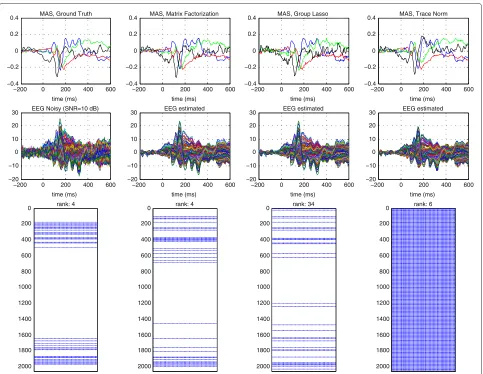
N=2, 052current sources within the brain, but only 40 of them are active: 4 main active sources with their corresponding 9 nearest neighbor sources are also active. The other 2012 sources are not active (zero electrical activity). Therefore, in this scenario, the synthetic matrixSis a structured sparse matrix with only 40 nonzero rows (the rows associated to the active sources).

In both scenarios, the simulated electrical activity (sim-ulated waveforms) associated to the four Main Active Sources (MAS) was obtained from a face perception-evoked potential study [35,36]. To obtain the simulated electrical activity associated to each one of the active neighbor sources, we simply set it as a scaled version of the electrical activity of its corresponding nearest MAS (with a scaled factor equal to 0.5). Hence, there is a linear relation between the four MAS and their corresponding nearest neighbor sources; therefore, in both scenarios, the rank of the synthetic matrixSis equal to 4.

As forward model (A), we used a three-shell concen-tric spherical head model. In this model, the inner sphere represents the brain, the intermediate layer represents the skull, and the outer layer represents the scalp [37]. To obtain the values of each one of the components of the matrixA, we need to solve the EEG forward problem [38]: Given the electrical activity of the current sources within the brain and a model for the geometry of the conducting media (brain, skull and scalp, with its corresponding elec-tric properties), compute the resulting EEG signals. This problem was solved by using the SPM software [39]. Tak-ing into account the comments mentioned in Section 2, the N simulated current sources were positioned on a mesh located on the brain cortex, with an orientation fixed perpendicular to it.

Finally, the simulated EEG signals were

gen-erated according to (1), where E is a Gaussian

noise G(0,σ2I) whose variance was set to satisfy a

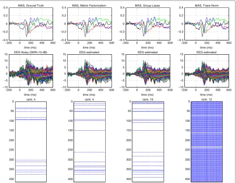
Y∈R128×161_andA∈R128×N_{, recover the synthetic BES} matrixS∈ RN×161. According to this, in both scenarios, we want to estimate a BES matrix which is structured sparse and low rank, with its rank equal to the number of MAS simulated. The activity of the four MAS, the syn-thetic EEG measurements as well as the sparsity pattern of the synthetic BES matrix are shown in Figures 1 and 2 (Ground Truth).

We have used cross-validation to select the regulariza-tion parameterλassociated to the Group Lasso and Trace Norm regularizers, as well as the parameters λ and K

in the case of the Matrix Factorization approach (K ∈

[1, 2, 3,. . ., 10],λ ∈[10−3, 10−2, 10−1,. . ., 103]): the rows ofYare randomly partitioned into three groups of approx-imately equal size. Each union of two groups forms a train set (TrS), while the remaining group forms a test set (TS). This procedure is carried out three times, each time selecting a different test group. Inverse reconstruc-tions are carried out based on the training sets, obtaining

different regression matricesSˆi. We then evaluate the root mean square error (RMSE) using the test sets and the regression matricesSˆi:

RMSE: 1

the index set of the rows that belongs to theith test set). Once the estimated matrixSˆ has been found, we apply a threshold to remove spurious sources with almost zero activity. We have set this threshold equal to the 1% of the mean energy of all the sources.

7.1 Performance evaluation

In order to evaluate the performance of the regulariz-ers, we compare the waveform and localization of the four MAS present in the synthetic BES matrix against the four MAS estimated by each one of the regularizers.

−200 0 200 400 600 −0.4

−0.2 0 0.2

0.4 MAS, Ground Truth

time (ms)

15 EEG Noisy (SNR=10 dB)

time (ms)

0.4 MAS, Matrix Factorization

time (ms)

0.4 MAS, Group Lasso

time (ms)

0.4 MAS, Trace Norm

time (ms)

−200 0 200 400 600 −0.4

−0.2 0 0.2

0.4 MAS, Ground Truth

time (ms)

30 EEG Noisy (SNR=10 dB)

time (ms)

0.4 MAS, Matrix Factorization

time (ms)

0.4 MAS, Group Lasso

time (ms)

0.4 MAS, Trace Norm

time (ms)

Figure 2Simulation results: waveforms of the MAS, EEG estimated, and sparsity pattern of the estimated BES matrix.Experiment setup: 2,052 sources, 128 EEG electrodes, 161 time instants, 4 main active sources with their corresponding 9 nearest neighbor sources also active.

We also compare the sparsity pattern of the estimated BES matrixSˆ against the sparsity pattern of the synthetic BES matrixS, as well as the synthetic and predicted EEG measurements.

As we can see from Figures 1 and 2, the Group Lasso and Trace Norm regularizers do not reveal the correct number of linear independent sources, while the Matrix Factorization does: it finds out four linear independent sources in both scenarios. To select such four linear inde-pendent MAS, we find a basis for the Column Space(S˜₎ (using a QR factorization), where S˜ is a matrix whose rows are a sorted version of the rows of S (sorted in a descending order of their corresponding energy value). To get the four linear independent MAS estimated by the Group Lasso and Trace Norm regularizers, we followed the same procedure described before and retained the first four components of the basis of the Column Space(S˜).

According to Figures 1 and 2, the Matrix Factorization approach is able to estimate a BES matrix with the correct

rank and whose sparsity pattern follows closely the spar-sity pattern of the true BES matrix, that is, both matrices have a similar structure, which implies that the proposed approach is able to induce the desired solution: A row-structured sparse matrix, whose nonzero rows encode the linear relation between the active sources and their cor-responding nearest neighbor sources. Using the estimated BES matrix, the Matrix Factorization approach is also able to predict a smooth version of the noisy EEG, and the waveforms of the estimated MAS follow closely the waveforms of the true MAS.

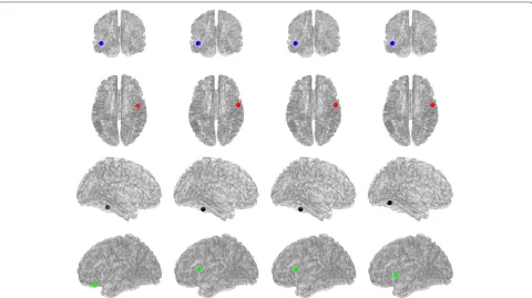
Figure 3Localization of the MAS,N=413sources.From left to right: Ground Truth, Matrix Factorization, Group Lasso, and Trace Norm.

As we can see from Figures 1 and 2, the Trace Norm regularizer takes into account the linear relation of the active sources by inducing solutions which are low rank, but, on the other hand, it does not take into account the structured sparsity pattern of the BES matrix. All of this implies that the Trace Norm tends to induce low rank dense solutions, which are not biologically plausible.

According to Figures 3 and 4, the position of the MAS obtained from the BES matrix estimated by the Matrix Factorization approach, the Group Lasso, and Trace Norm regularizers follows closely the position of the true MAS. Nevertheless, it is worth highlighting that before selecting the MAS, we first need an accurate esti-mation of their number, and the Group Lasso and Trace Norm regularizers were not able to get a precise estimate of it, only the Matrix Factorization were able to.

From these results, we can see that the proposed Matrix Factorization approach outperforms both the Group Lasso and Trace Norm regularizers. The main reason for this is because it combines their two main features: it com-bines the structured sparsity (from Group Lasso) and the low rank (from Trace Norm) into one unified framework, which implies that it is able to induce structured sparse-low-rank solutions which are biologically plausible: few active sources, with linear relations between them.

8 Conclusions

We have presented a novel approach to solve the EEG inverse problem, which is based on matrix factoriza-tion and regularizafactoriza-tion. Our method combines the ideas behind the Group Lasso (structured sparsity) and Trace Norm (low rank) regularizers into one unified framework. We have also developed and analyzed the convergence of an alternating minimization algorithm to solve the resulting nonsmooth-nonconvex regularization problem. Finally, using simulation studies, we have compared our method with the Group Lasso and Trace Norm regulariz-ers when they are applied directly to the target matrix, and we have shown the gain in performance obtained by our method, hence proving the effectiveness and efficiency of the proposed algorithm.

Competing interests

The authors declare that they have no competing interests.

Acknowledgements

The authors would like to thank the anonymous reviewers for their valuable comments and suggestions to improve the quality of the paper. They are also grateful to Dr. Carsten Stahlhut, from DTU Informatics, for valuable discussions about EEG brain imaging and also to Dr. Alexandre Gramfort, from Telecom ParisTech, for his advices related with EEG signal processing and nonsmooth convex programming theory applied to the EEG inverse problems. This work has been partly supported by Ministerio de Economía of Spain (projects ‘DEIPRO’ (id. TEC2009-14504-C02-01) and ‘COMONSENS’ (id. CSD2008-00010), ‘ALCIT’ (id. TEC2012-38800-C03-01), and ‘COMPREHENSION’ (id.

TEC2012-38883-C02-01)). Authors LKH and MP were funded by Banco Santander and Universidad Carlos III de Madrid’s Excellence Chair programme.

Author details

1_{Department of Signal Processing and Communications, Universidad Carlos III}

de Madrid, Avda. Universidad 30, Leganés, Madrid 28911, Spain.2_Department

of Computer Science, University College London, Gower Street, London WC1E 6BT, UK.3_{DTU Informatics, Cognitive Systems Section, Technical University of}

Denmark, Kongens Lyngby 2800, Denmark.

Received: 27 March 2014 Accepted: 16 June 2014 Published: 24 June 2014

References

1. M Hämäläinen, R Hari, RJ Ilmoniemi, J Knuutila, OV Lounasmaa, Magnetoencephalography—theory, instrumentation, and applications to noninvasive studies of the working human brain. Rev. Mod. Phys. 65(2), 413 (1993)

2. RD Pascual-Marqui, Review of methods for solving the EEG inverse problem. Int. J. Bioelectromagnetism1(1), 75–86 (1999)

3. S Baillet, JC Mosher, RM Leahy, Electromagnetic brain mapping. IEEE Signal Process. Mag.18(6), 14–30 (2001)

4. R Grech, T Cassar, J Muscat, KP Camilleri, SG Fabri, M Zervakis, P Xanthopoulos, V Sakkalis, B Vanrumste, Review on solving the inverse problem in EEG source analysis. J. Neuroeng. Rehabil.5(1), 25 (2008) 5. A Beck, M Teboulle, A fast iterative shrinkage-thresholding algorithm for

linear inverse problems. SIAM J. Imaging Sci.2(1), 183–202 (2009) 6. RGdP Menendez, MM Murray, CM Michel, R Martuzzi, SLG Andino,

Electrical neuroimaging based on biophysical constraints. NeuroImage 21(2), 527–539 (2004)

7. MS Hämäläinen, R Ilmoniemi, Interpreting magnetic fields of the brain: minimum norm estimates. Med. Biol. Eng. Comput.32(1), 35–42 (1994) 8. K Uutela, M Hämäläinen, E Somersalo, Visualization of

magnetoencephalographic data using minimum current estimates. NeuroImage10(2), 173–180 (1999)

9. W Ou, MS Hämäläinen, P Golland, A distributed spatio-temporal EEG/MEG inverse solver. NeuroImage44(3), 932–946 (2009)

10. A Gramfort, D Strohmeier, J Haueisen, M Hamalainen, M Kowalski, Functional brain imaging with M/EEG using structured sparsity in time-frequency dictionaries, inInformation Processing in Medical Imaging, Lecture Notes in Computer Science, ed. by G Székely, HK Hahn, vol. 6801 (Springer, Berlin, 2011), pp. 600–611

11. A Gramfort, D Strohmeier, J Haueisen, M Hämäläinen, M Kowalski, Time-Frequency Mixed-Norm Estimates: Sparse M/EEG imaging with non-stationary source activations. NeuroImage70, 410–22 (2013) 12. S Haufe, R Tomioka, T Dickhaus, C Sannelli, B Blankertz, G Nolte, KR Müller,

Large-scale EEG/MEG source localization with spatial flexibility. NeuroImage54(2), 851–859 (2011)

13. A Gramfort, M Kowalski, M Hämäläinen, Mixed-norm estimates for the M/EEG inverse problem using accelerated gradient methods. Phys. Med. Biol.57(7), 1937 (2012)

14. F Bach, R Jenatton, J Mairal, G Obozinski, Optimization with Sparsity-Inducing Penalties. Foundations Trends® Mach. Learn. 4(1), 1–106 (2011)

15. CA Micchelli, JM Morales, M Pontil, Regularizers for structured sparsity. Adv. Comput. Math.38(3), 455–489 (2013)

16. S Sra, S Nowozin, SJ Wright,Optimization for Machine Learning(MIT Press, Cambridge, 2012)

17. DP Bertsekas,Nonlinear Programming(Athena Scientific, Belmont, 1999) 18. PL Combettes, VR Wajs, Signal recovery by proximal forward-backward

splitting. Multiscale Model. Simul.4(4), 1168–1200 (2005) 19. PL Combettes, J-C Pesquet, Proximal splitting methods in signal

processing, inFixed-Point Algorithms for Inverse Problems in Science and Engineering, Springer Optimization and Its Applications, ed. by HH Bauschke, RS Burachik, PL Combettes, V Elser, DR Luke, and H Wolkowicz, vol. 49 (Springer New York, 2011), pp. 185–212

20. Y Nesterov, Gradient methods for minimizing composite objective function. CORE Discussion Papers 2007076, Center for Operations Research and Econometrics (CORE), Université Catholique de Louvain (2007)

23. J Malmivuo, R Plonsey,Bioelectromagnetism: Principles and Applications of Bioelectric and Biomagnetic Fields(Oxford University Press, Oxford, 1995) 24. S Murakami, Y Okada, Contributions of principal neocortical neurons to magnetoencephalography and electroencephalography signals. J Phys. 575(3), 925–936 (2006)

25. JJ Moreau, Proximité et dualité dans un espace hilbertien. Bull. Soc. Math. France93(2), 273–299 (1965)

26. CA Micchelli, L Shen, Y Xu, Proximity algorithms for image models: denoising. Inverse Probl.27, 045009 (2011)

27. M Schmidt, NL Roux, F Bach, Convergence rates of inexact

proximal-gradient methods for convex optimization. Adv. Neural Inform. Process. Syst.24, 1458–1466 (2011)

28. A Argyriou, T Evgeniou, M Pontil, Convex multi-task feature learning. Mach. Learn.73(3), 243–272 (2008)

29. RA Horn, CR Johnson,Matrix Analysis(Cambridge university press, Cambridge, 1990)

30. WI Zangwill,Nonlinear Programming: a Unified Approach. (Prentice-Hall, Englewood Cliffs, 1969)

31. B Sriperumbudur, G Lanckriet, On the convergence of the concave-convex procedure. Adv. Neural Inform. Process. Syst. 22, 1759–1767 (2009)

32. A Gunawardana, W Byrne, Convergence theorems for generalized alternating minimization procedures. J. Mach. Learn. Res.6, 2049–2073 (2005)

33. R Jenatton, J Mairal, G Obozinski, F Bach, Proximal methods for sparse hierarchical dictionary learning, inProceedings of the International Conference on Machine Learning (ICML)(Haifa, 21–24 June 2010) 34. J Mairal, R Jenatton, FR Bach, GR Obozinski, Network flow algorithms for

structured sparsity. Adv. Neural Inform. Process. Syst.23, 1558–1566 (2010) 35. K Friston, L Harrison, J Daunizeau, S Kiebel, C Phillips, N Trujillo-Barreto, R

Henson, G Flandin, J Mattout, Multiple sparse priors for the M/EEG inverse problem. NeuroImage39(3), 1104–1120 (2008)

36. R Henson, Y Goshen-Gottstein, T Ganel, L Otten, A Quayle, M Rugg, Electrophysiological and haemodynamic correlates of face perception, recognition and priming. Cereb. Cortex.13(7), 793 (2003)

37. H Hallez, B Vanrumste, R Grech, J Muscat, W De Clercq, A Vergult, Y D’Asseler, KP Camilleri, SG Fabri, S Van Huffel, I Lemahieu, Review on solving the forward problem in EEG source analysis. J. Neuroeng. Rehabil. 4(1), 46 (2007)

38. JC Mosher, RM Leahy, PS Lewis, EEG and MEG: forward solutions for inverse methods. IEEE Trans. Biomed. Eng.46(3), 245–259 (1999) 39. V Litvak, J Mattout, S Kiebel, C Phillips, R Henson, J Kilner, G Barnes, R

Oostenveld, J Daunizeau, G Flandin, W Penny, K Friston, EEG and MEG data analysis in SPM8. Comput. Intell. Neurosci (2011).

doi:10.1155/2011/852961

doi:10.1186/1687-6180-2014-97

Cite this article as:Montoya-Martínezet al.:A regularized matrix factorization approach to induce structured sparse-low-rank solutions in

the EEG inverse problem.EURASIP Journal on Advances in Signal Processing

20142014:97.

Submit your manuscript to a

journal and benefi t from:

7Convenient online submission 7Rigorous peer review

7Immediate publication on acceptance 7Open access: articles freely available online 7High visibility within the fi eld

7Retaining the copyright to your article