A Generalized Algorithm for the Generation
of Correlated Rayleigh Fading Envelopes
in Wireless Channels
Le Chung Tran
Telecommunications and Information Technology Research Institute (TITR), School of Electrical, Computer and Telecommunications Engineering, University of Wollongong, Wollongong NSW 2522, Australia
Email:[email protected]
Tadeusz A. Wysocki
School of Electrical Computer and Telecommunications Engineering, Faculty of Informatics, University of Wollongong, Wollongong NSW 2522, Australia
Email:[email protected]
Alfred Mertins
Signal Processing Group, Department of Physics, University of Oldenburg, 26111 Oldenburg, Germany Email:[email protected]
Jennifer Seberry
School of Information Technology and Computer Science, Faculty of Informatics, University of Wollongong, Wollongong NSW 2522, Australia
Email:[email protected]
Received 23 January 2005; Revised 6 July 2005; Recommended for Publication by Wei Li
Although generation of correlated Rayleigh fading envelopes has been intensively considered in the literature, all conventional methods have their own shortcomings, which seriously impede their applicability. A very general, straightforward algorithm for the generation of anarbitrarynumber of Rayleigh envelopes withany desired,equal or unequalpower, in wireless channels either withorwithoutDoppler frequency shifts, is proposed. The proposed algorithm can be applied to the case ofspatial correlation, such as with multiple antennas in multiple-input multiple-output (MIMO) systems, orspectral correlationbetween the random pro-cesses like in orthogonal frequency-division multiplexing (OFDM) systems. It can also be used for generating correlated Rayleigh fading envelopes in eitherdiscrete-time instantsor areal-time scenario. Besides beingmore generalized, our proposed algorithm is more precise, while overcoming all shortcomings of the conventional methods.
Keywords and phrases:correlated Rayleigh fading envelopes, antenna arrays, OFDM, MIMO, Doppler frequency shift.
1. INTRODUCTION
In orthogonal frequency-division multiplexing (OFDM) sys-tems, the fading affecting carriers may have cross-correlation due to the small coherence bandwidth of the channel, or due to the inadequate frequency separation between the carriers. In addition, in multiple-input multiple-output (MIMO) sys-tems where multiple antennas are used to transmit and/or
This is an open access article distributed under the Creative Commons Attribution License, which permits unrestricted use, distribution, and reproduction in any medium, provided the original work is properly cited.
receive signals, the fading affecting these antennas may also experience cross-correlation due to the inadequate separa-tion between the antennas. Therefore, a generalized, straight-forward and, certainly, correct algorithm to generate corre-lated Rayleigh fading envelopes is required for the researchers wishing to analyze theoretically and simulate the perfor-mance of systems.
shortcomings which seriously limit their applicability or even cause failures in generating the desired Rayleigh fading en-velopes.
In this paper, we modify existing methods and propose a generalized algorithm for generating correlated Rayleigh fad-ing envelopes. Our modifications are simple, butimportant and also veryefficient. The proposed algorithm thus incor-porates the advantages of the existing methods, while over-coming all of their shortover-comings. Furthermore, besides being more generalized, the proposed algorithm ismore accurate, while providing more useful featuresthan the conventional methods.
The paper is organized as follows. InSection 2, a sum-mary of the shortcomings of conventional methods for gen-erating correlated Rayleigh fading envelopes is derived. In Sections3.1 and3.2, we shortly review the discussions on the correlation property between the transmitted signals as functions of time delay and frequency separation, such as in OFDM systems, and as functions of spatial separation be-tween transmission antennas, such as in MIMO systems, re-spectively. InSection 4, we propose a very general, straight-forward algorithm to generate correlated Rayleigh fading en-velopes.Section 5derives an algorithm to generate correlated Rayleigh fading envelopes in a real-time scenario. Simulation results are presented inSection 6. The paper is concluded by
Section 7.
2. SHORTCOMINGS OF CONVENTIONAL METHODS AND AIMS OF THE PROPOSED ALGORITHM
We first analyze the shortcomings of some conventional methods for the generation of correlated Rayleigh fading en-velopes.
In [3], the authors derived fading correlation proper-ties in antenna arrays and, then, briefly mentioned the algo-rithm to generate complex Gaussian random variables (with Rayleigh envelopes) corresponding to a desired correlation coefficient matrix. This algorithm was proposed for gener-atingequal powerRayleigh envelopes only, rather than arbi-trary(equal or unequal) power Rayleigh envelopes.
In [4, 5], the authors proposed different methods for
generating onlyN =2equal powercorrelated Rayleigh en-velopes. In [6], the authors generalized the method of [5] for
N ≥ 2. However, in this method, Cholesky decomposition [7] is used, and consequently, the covariance matrix must be positive definite, which is not always realistic. An example, where the covariance matrix is not positive definite, is de-rived later inExample 1ofSection 4.1of this paper.
These methods were then more generalized in [8], where one can generate any numberof Rayleigh envelopes corre-sponding to a desired covariance matrix and withany power, that is, even withunequalpower. However, again, the covari-ance matrix must be positive definite in order for Cholesky decomposition to be performable. In addition, the authors in [8] forced the covariances of the complex Gaussian random variables (with Rayleigh fading envelopes) to bereal(see [8, (8)]). This limitation prohibits the use of their method in
various cases because, in fact, the covariances of the plex Gaussian random variables are more likely to be com-plex.
In [2], the authors proposed a method for generating any numberof Rayleigh envelopes withequal poweronly. Al-though the method of [2] works well in various cases, itfails to perform Cholesky decomposition for some complex co-variance matrices in Matlab due to the roundofferrors of Matlab.1 This shortcoming is overcome by some
modifica-tions mentioned later in our proposed algorithm.
More importantly, the method proposed in [2]failsto generate Rayleigh fading envelopes corresponding to a de-sired covariance matrix in a real-time scenariowhere Doppler frequency shifts are considered. This is because passing Gaus-sian random variables with variances assumed to be equal to one (for simplicity of explanation) through a Doppler fil-ter changes remarkably the variances of those variables. The variances of the variables at the outputs of Doppler filters are notequal to one any more, but depend on the variance of the variables at the inputs of the filters as well as the character-istics of those filters. The authors in [2] did not realize this variance-changing effect caused by Doppler filters. We will return to this issue later in this paper.
For the aforementioned reasons, amore generalized algo-rithm is required to generateany numberof Rayleigh fading envelopes with any power (equal or unequal power) corre-sponding to any desired covariance matrix. The algorithm should be applicable to both discrete time instant scenario and real-time scenario. The algorithm is also expected to overcome roundoff errors which may cause the interrup-tion of Matlab programs. In addiinterrup-tion, the algorithm should work well, regardless of the positive definiteness of the co-variance matrices. Furthermore, the algorithm should pro-vide a straightforward method for the generation of com-plex Gaussian random variables (with Rayleigh envelopes) with correlation properties as functions of time delay and frequency separation(such as in OFDM systems), orspatial separation between transmission antennas (like with multi-ple antennas in MIMO systems). This paper proposes such an algorithm.
3. BRIEF REVIEW OF STUDIES ON FADING CORRELATION CHARACTERISTICS
In this section, we shortly review the discussions on the cor-relation property between the transmitted signals as
func-1It has been well known that Cholesky decomposition may not work for the matrix having eigenvalues being equal or close to zeros. We consider the following covariance matrixK, for instance:
K=
1.04361 0.7596−0.3840i 0.6082−0.4427i 0.4085−0.8547i 0.7596 + 0.3840i 1.04361 0.7780−0.3654i 0.6082−0.4427i 0.6082 + 0.4427i 0.7780 + 0.3654i 1.04361 0.7596−0.3840i 0.4085 + 0.8547i 0.6082 + 0.4427i 0.7596 + 0.3840i 1.04361
.
tions of time delay and frequency separation, such as in OFDM systems, and as functions of spatial separation be-tween transmission antennas, such as in MIMO systems. These discussions were originally derived in [3,9], respec-tively.
This review aims at facilitating readers to apply our pro-posed algorithm in different scenarios (i.e.,spectral correla-tion, such as in OFDM systems, orspatial correlation, such as in MIMO systems) as well as pointing out the condition for the analyses in [3,9] to be applicable to our proposed al-gorithm (i.e., these analyses are applicable to our alal-gorithm if the powers (variances) of different random processes are assumed to be the same).
3.1. Fading correlation as functions of time delay and frequency separation
In [9], Jakes considered the scenario where all complex Gaus-sian random processes with Rayleigh envelopes have equal powers σ2 and derived the correlation properties between
random processes as functions of both time delay and fre-quency separation, such as in OFDM systems. Letzk(t) and zj(t) be the two zero-mean complex Gaussian random pro-cesses at time instantt, corresponding to frequencies fkand
fj, respectively. Denote
xkRe
zk(t)
, ykIm
zk(t)
,
xjRe
zj
t+τk,j
, yjIm
zj
t+τk,j
, (1)
whereτk,j is the arrival time delay between two signals and Re(·), Im(·) are the real and imaginary parts of the argu-ment, respectively. By definition, the covariances between the real and imaginary parts ofzk(t) andzj(t+τk,j) are
Rxxk,j E
xkxj
, Ry y k,jEykyj
,
Rxy k,jExkyj
, Ryxk,jEykxj
.
(2)
Then, those covariances have been derived in [9, (1.5-20)] as
Rxxk,j=Ry y k,j= σ2J
0
2πFmτk,j
2 1 +∆ωk,jστ
2,
Rxy k,j= −Ryxk,j= −∆ωk,jστRxxk,j,
(3)
where σ2 is the variance (power) of the complex Gaussian
random processes (σ2/2 is the variance per dimension);J 0
is the first-kind Bessel function of the zeroth-order; Fm is the maximum Doppler frequency Fm = v/λ = v fc/c. In this formula,λis the wavelength of the carrier, fcis the car-rier frequency, cis the speed of light, and v is the mobile speed; ∆ωk,j = 2π(fk− fj) is the angular frequency sep-aration between the two complex Gaussian processes with Rayleigh envelopes at frequencies fk and fj;στ is the root-mean-square (rms) delay spread of the wireless channel.
∆ ∆ Receiver
Φ
K Transmit antennas
Tx−1 Tx D
1 2
Figure1: Model to examine the spatial correlation between
trans-mitter antennas.
It should be emphasized that, the equalities (3) hold only when the set ofmultipath channel coefficients, which were de-noted asCnmand derived in [9, (1.5-1) and (1.5-2)], as well as thepowersare assumed to be thesamefor different random processes (with different frequencies). Readers may refer to [9, pages 46–49] for an explicit exposition.
3.2. Fading correlation as functions of spatial separation in antenna arrays
The fading correlation properties between wireless channels as functions of antenna spacing in multiple antenna sys-tems have been mentioned in [3].Figure 1presents a typ-ical model of the channel where all signals from a receiver are assumed to arrive atTx antennas within±∆at angleΦ (|Φ| ≤π). Letλbe the wavelength,Dthe distance between the two adjacent transmitter antennas, and z = 2π(D/λ). In [3], it is assumed that fading corresponding to different receivers is independent. This is reasonable if receivers are not on top of each other within some wavelengths and they are surrounded by their own scatterers. Consequently, we only need to calculate the correlation properties for a typi-cal receiver. The fading in the channel between a given kth transmitter antenna and the receiver may be considered as a zero-mean, complex Gaussian random variable, which is presented asb(k) =x(k)+iy(k). Denote the covariances
be-tween the real parts as well as the imaginary parts them-selves of the fading corresponding to thekth and jth trans-mitter antennas2 to beR
xxk,j andRy y k,j, while those terms between the real and imaginary parts of the fading to be
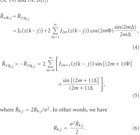
Rxy k,j andRyxk,j. The termsRxxk,j,Ry y k,j,Rxy k,j, andRyxk,j are similarly defined as (2). Then, it has been proved that the closed-form expressions of these covariances normalized by the variance per dimension (real and imaginary) are (see [3,
(A. 19) and (A. 20)])
In these equations,Jqis the first-kind Bessel function of the integer order q, and σ2/2 is the variance per dimension of
the received signal at each transmitter antenna, that is, it is assumed in [3] that the signals corresponding to different transmitter antennas haveequalvariancesσ2.
Similarly toSection 3.1, the equalities (4) and (5) hold only when the set of multipath channel coefficients, which were denoted asgnand derived in [3, (A-1)], and thepowers are assumed to be thesamefor different random processes. Readers may refer to [3, pages 1054–1056] for an explicit ex-position.
4. GENERALIZED ALGORITHM TO GENERATE
CORRELATED, FLAT RAYLEIGH FADING ENVELOPES
4.1. Covariance matrix of complex Gaussian random variables with Rayleigh fading envelopes
It is known that Rayleigh fading envelopes can be gener-ated from zero-mean, complex Gaussian random variables. We consider here a column vectorZofNzero-mean, com-plexGaussian random variables with variances (or powers)
σg2j, for j = 1,. . .,N. DenoteZ = (z1,. . .,zN)T, where zj the phases θj’s are independent, identically uniformly dis-tributed random variables. As a result, the real and imaginary parts of eachzjare independent (butzj’s are not necessarily independent), that is, the covariancesE(xjyj)=0 for for all
jand therefore,rj’s areRayleigh envelopes. Letσ2
gx jandσ
2
gy jbe the variances per dimension (real and imaginary), that is,σ2
gx j=E(x a very general scenario where the variances (powers) of the real parts are not necessarily equal to those of the imaginary parts. Also, the powers of Rayleigh envelopes denoted asσ2
rj are not necessarily equal to one another. Therefore, the sce-nario where the variances of the Rayleigh envelopes are equal to one another and the powers of real parts are equal to those of imaginary parts, such as the scenario mentioned in either
Section 3.1orSection 3.2, is considered as a particular case. Fork= j, we define the covariancesRxxk,j,Ry y k,j,Rxy k,j, andRyxk,j between the real as well as imaginary parts ofzk andzj, similarly to those mentioned in (2).
By definition, the covariance matrixKofZis
K=EZZHµ k,j
N×N, (8)
where (·)H denotes the Hermitian transposition operation and
In reality, the covariance matrixKisnotalways positive semidefinite. An example where the covariance matrixKis notpositive semidefinite is derived as follows.
Example 1. We examine an antenna array comprising 3 transmitter antennas. LetDk j, fork,j =1,. . ., 3, be the dis-tance between thekth antenna and thejth antenna. The dis-tanceDjk between jth antenna and thekth antenna is then Djk= −Dk j. Specifically, we consider the case
D21=0.0385λ,
D31=0.1789λ,
D32=0.1560λ,
(10)
whereλis the wavelength. Clearly, these antennas areneither equally spaced,norpositioned in a straight line. Instead, they are positioned at the 3 peaks of a triangle.
If the receiver antenna is far enough from the transmit-ter antennas, we can assume that all signals from the receiver arrive at the transmitter antennas within±∆at angleΦ(see
Figure 1for the illustration of these notations). As a result, the analytical results mentioned in Section 3.2 with small modifications can still be applied to this case. In particular, covariance matrixKcan still be calculated following (4), (5), (6), (8), and (9), provided that, in (4) and (5), the products
z(k−j) (or 2πD(k−j)/λ) are replaced by 2πDk j/λ. This is because, in our considered case,Dk j are the actual distances between thekth transmitter antenna and thejth transmitter antenna, fork,j=1,. . ., 3.
Further, we assume that the varianceσ2 of the received
signals at each transmitter antenna in (6) is unit, that is,σ2=
1. We also assume thatΦ =0.1114πrad and∆=0.1114π
In order to examine the performance of the considered system, the Rayleigh fading envelopes are required to be sim-ulated. In turn, the covariance matrix of the complex Gaus-sian random variables corresponding to these Rayleigh en-velopes must be calculated. Based on the aforementioned as-sumptions, from the theoretically analytical equations (4), (5), and (6), and the definition equations (8) and (9), we have the following desired covariance matrix for the considered configuration of transmitter antennas:
K=
0.99571.0000−0.0811i 0.9957 + 01.0000.0811i 00..9090 + 09303 + 0..31803607ii
0.9090−0.3607i 0.9303−0.3180i 1.0000
.
(11)
Performing eigen decomposition, we have the following eigenvalues:−0.0092; 0.0360; and 2.9733. Therefore,Kisnot positive semidefinite. This also means thatK isnotpositive definite.
It is important to emphasize that, from the mathemat-ical point of view, covariance matrices are alwayspositive semidefinite by definition (8), that is, the eigenvalues of the covariance matrices areeitherzeroorpositive. However, this does not contradict the above example where the covariance matrix K has a negative eigenvalue. The main reason why the desired covariance matrixKis not positive semidefinite is due to the approximation and the simplifications of the model mentioned in Figure 1in calculating the covariance values, that is, due to the preciseness of (4) and (5), com-pared to the true covariance values. In other words, errors in estimating covariance values may exist in the calculation. Those errors may result in a covariance matrix being not pos-itive semidefinite.
A question that could be raised here is why the covari-ance matrix of complex Gaussian random variables (with Rayleigh fading envelopes), rather than the covariance ma-trix ofRayleigh envelopes, is of particular interest. This is due to the two following reasons.
From the physical point of view, in the covariance ma-trix ofRayleigh envelopes, the correlation propertiesRxx,Ry y of the real components (inphase components) as well as the imaginary components (quadrature phase components) themselves and the correlation propertiesRxy,Ryx between the real and imaginary components of random variables are notdirectly present (these correlation properties are defined in (2)). On the contrary, those correlation properties are clearly present in the covariance matrix of complex Gaus-sian random variables with the desired Rayleigh envelopes. In other words, the physical significance of the correlation properties of random variables isnotpresent as detailed in the covariance matrix ofRayleigh envelopesas in the covari-ance matrix of complex Gaussian random variables with the desired Rayleigh envelopes.
Further, from the mathematical point of view, it is pos-sible to have one-to-one mappingfromthe cross-correlation coefficientsρgi j (between theith and jth complex Gaussian random variables) to the cross-correlation coefficients ρri j
(between Rayleigh fading envelopes) as follows (see [9, (1.5-26)]):
ρri j =
1 +ρgi jEint
2ρgi j/
1 +ρgi j−π/2
2−π/2 , (12)
whereEint(·) is the complete elliptic integral of the second
kind. Some good approximations of this relationship be-tween ρri j andρgi j are presented in the mapping [4, Table II], the look-up [8, Table I and Figure 1].
However, the reversed mapping, that is, the mapping from ρri j to ρgi j, is multivalent. It means that, for a given ρri j, we have to somehow determineρgi j in order to gener-ate Rayleigh fading envelopes and the possible values ofρgi j may be significantly different from each other depending on howρgi jis determined fromρri j. It is noted thatρri jis always real, butρgi jmay be complex.
For the two aforementioned reasons, the covariance ma-trix of complex Gaussian random variables (with Rayleigh envelopes), as opposed to the covariance matrix of Rayleigh envelopes, is of particular interest in this paper.
4.2. Forced positive semidefiniteness of the covariance matrix
First, we need to define thecoloring matrixLcorresponding to a covariance matrixK. Thecoloring matrixLis defined to be theN×Nmatrix satisfying
LLH=K. (13)
It is noted that the coloring matrix isnotnecessarily a lower triangular matrix. Particularly, to determine the coloring ma-trixLcorresponding to a covariance matrixK, we can use eitherCholesky decomposition [7] as mentioned in a num-ber of papers, which have been reviewed inSection 2of this paper, or eigen decomposition which is mentioned in the next section of this paper. The former yields a lower trian-gular coloring matrix, while the later yields a square coloring matrix.
Unlike Cholesky decomposition, where the covariance matrixKmust bepositive definite, eigen decomposition re-quires thatKis at leastpositive semidefinite, that is, the eigen-values ofKare either zeros or positive. We will explain later why the covariance matrix must be positive semidefinite even in the case where eigen decomposition is used to calculate the coloring matrix. The covariance matrixK, in fact, maynot be positive semidefinite, that is,Kmay have negative eigen-values, as the case mentioned inExample 1ofSection 4.1.
out if all eigenvalues are positive. Our procedure is presented as follows.
Assuming thatKis the desired covariance matrix, which is not positive semidefinite, perform the eigen decomposi-tion K = VGVH, where V is the matrix of eigenvectors andGis a diagonal matrix of eigenvalues of the matrixK. LetG=diag(λ1,. . .,λN). Calculate the approximate matrix Λdiag( ˆλ1,. . ., ˆλN), where
ˆ
λj=
λj ifλj≥0,
0 ifλj<0.
(14)
We now compare our approximation procedure to the ap-proximation procedure mentioned in [2]. The authors in [2] used the following approximation:
ˆ
λj=
λj ifλj>0,
ε ifλj≤0,
(15)
whereεis a small, positive real number.
Clearly, besides overcoming the disadvantage of Cholesky decomposition, our approximation procedure ismore precise under realistic assumptions like finite precision arithmetic than the one mentioned in [2], since the matrix Λ in our algorithm approximates to the matrixGbetter than the one mentioned in [2]. Therefore, the desired covariance matrix
K is well approximated by the positive semidefinite matrix K=VΛVHfrom Frobenius point of view [2].
4.3. Determine the coloring matrix using eigen decomposition
In most of the conventional methods, Cholesky decomposi-tion was used to determine the coloring matrix. As analyzed earlier inSection 2, Cholesky decomposition may not work for the covariance matrix which has eigenvalues being equal or close to zeros.
To overcome this disadvantage, we use eigen decom-position, instead of Cholesky decomdecom-position, to calculate the coloring matrix. Comparison of the computational ef-forts between the two methods (eigen decomposition versus Cholesky decomposition) is mentioned later in this paper. The coloring matrix is calculated as follows.
At this stage, we have the forced positive semidefinite covariance matrix K, which is equal to the desired covari-ance matrix K if K is positive semidefinite, or approxi-mates to K otherwise. Further, as mentioned earlier, we have K = VΛVH, where Λ = diag( ˆλ
1,. . ., ˆλN) is the ma-trix of eigenvalues of K. Since K is a positive semidefi-nite matrix, it follows that {λˆj}N
j=1 are real and
nonnega-tive.
We now calculate a new matrix ¯Λas
¯
Λ=Λ=diag
ˆ
λ1,. . .,
ˆ
λN
. (16)
Clearly, ¯Λis areal,diagonalmatrix that results in
¯
ΛΛ¯H=Λ¯Λ¯ =Λ. (17)
If we denoteLVΛ, then it follows that¯
LLH=(VΛ)(V¯ Λ)¯ H=VΛ¯Λ¯HVH=VΛVH=K. (18)
It means that the coloring matrixLcorresponding to the co-variance matrixKcan be computedwithoutusing Cholesky decomposition. Thereby, the shortcoming of [2], which is re-lated to roundofferrors in Matlab caused by Cholesky de-composition and is pointed out in Section 2, can be over-come.
We now explain why the covariance matrix must be pos-itive semidefinite even when eigen decomposition is used to compute the coloring matrix. It is easy to realize that, ifK isnotpositive semidefinite covariance matrix, then ¯Λ calcu-lated by (16) is acomplexmatrix. As a result, (17) and (18) are not satisfied.
4.4. Proposed algorithm
In Section 2, we have shown that the method proposed in [2] fails to generate Rayleigh fading envelopes corresponding to a desired covariance matrix in a real-time scenario where Doppler frequency shifts are considered. This is because the authors in [2] did not realize the variance-changing effect
caused by Doppler filters.
To surmount this shortcoming, the two followingsimple, but importantmodifications must be carried out.
(1) Unlike step 6 of the method in [2], where N inde-pendent, complex Gaussian random variables (with Rayleigh fading envelopes) are generated with unit variances, in our algorithm, this step is modified in order to be able to generate independent, complex Gaussian random variables with arbitrary variances
σ2
g. Correspondingly, step 7 of the method in [2] must also be modified. Besides being more generalized, the modification of our algorithm in steps 6 and 7 allows us to combine correctly the outputs of Doppler filters in the method proposed in [10] and our algorithm. (2) The variance-changing effect of Doppler filters must
be considered. It means that, we have to calculate the variance of the outputs of Doppler filters, which may have anarbitraryvalue depending on the variance of the complex Gaussian random variables at the inputs of Doppler filters as well as the characteristics of those filters. The variance value of the outputs is then input into the step 6 which has been modified as mentioned above.
Doppler frequency shifts are considered (see the algorithm mentioned inSection 5).
From the above observations, we propose here a gener-alized algorithm to generateNcorrelated Rayleigh envelopes in asingle time instantas given below.
(1) In a general case, the desired variances (powers) {σ2
gj} N
j=1 of complex Gaussian random variables with
Rayleigh envelopes must be known. Specially, if one wants to generate Rayleigh envelopes corresponding to the desired variances (powers){σ2
rj} N
j=1, then{σg2j} N j=1
are calculated as follows:3
σ2
(2) From the desired correlation properties of correlated complex Gaussian random variables with Rayleigh en-velopes, determine the covariancesRxxk,j,Ry y k,j,Rxy k,j andRyxk,j, fork,j = 1,. . .,N andk = j. In other words, in a general case, those covariances must be known. Specially, in the case where the powers of all random processes areequaland other conditions hold as mentioned in Sections3.1and3.2, we can follow (3) in the case of time delay and frequency separation, such as in OFDM systems, or (4), (5), and (6) in the case of spatial separation like with multiple antennas in MIMO systems to calculate the covariancesRxxk,j,
Ry y k,j, Rxy k,j, and Ryxk,j. The values {σ2
gj} N
j=1,Rxxk,j,
Ry y k,j,Rxy k,j, andRyxk,j (k,j = 1,. . .,N;k = j) are the input data of our proposed algorithm.
(3) Create theN×N-sized covariance matrixK:
K=µk,j
The covariance matrix of complex Gaussian random variables is considered here, as opposed to the covari-ance matrix of Rayleigh fading envelopes like in the conventional methods.
(4) Perform the eigen decomposition:
K=VGVH. (22)
DenoteG diag(λ1,. . .,λN). Then, calculate a new
3Note thatσ2
gj is the variance ofcomplexGaussian random variables, rather than the variance per dimension (real or imaginary). Hence, there is no factor of 2 in the denominator.
diagonal matrix:
Thereby, we have a diagonal matrixΛwith all elements in the main diagonal beingrealand definitely nonneg-ative.
(5) Determine a new matrix ¯Λ = √Λ and calculate the coloring matrixLby settingL=VΛ¯.
(6) Generate a column vectorWofN independent com-plex Gaussian random samples with zero means and arbitrary, equalvariancesσ2
g:
W=u1,. . .,uN
T
. (25)
We can see that the modification (1) takes place in this step of our algorithm and proceeds in the next step. (7) Generate a column vectorZofN correlatedcomplex
Gaussian random samples as follows:
Z=LW
As shown later in the next section, the elements{zj}N j=1
are zero-mean, (correlated) complex Gaussian ran-dom variables with variances{σ2
gj} N
j=1. TheNmoduli
{rj}N
j=1 of the Gaussian samples inZare the desired
Rayleigh fading envelopes.
4.5. Statistical properties of the resultant envelopes
In this section, we check the covariance matrix and the vari-ances (powers) of the resultant correlated complex Gaussian random samples as well as the variances (powers) of the re-sultant Rayleigh fading envelopes.
It is easy to check thatE(WWH)=σ2
It means that the generated Rayleigh envelopes are corre-sponding to the forced positive semidefinite covariance ma-trixK, which is, in turn,equalto the desired covariance ma-trixKin caseKispositive semidefinite, orwell approximates toKotherwise. In other words, the desired covariance ma-trixKof complex Gaussian random variables (with Rayleigh fading envelopes) is achieved.
main diagonal ofKare thus equal (or close) toσ2
gj’s (see (20) and (21)). As a result, the resultant complex Gaussian ran-dom variables{zj}N
j=1 inZhave zero means and variances
(powers){σ2
gj} N j=1.
It is known that the means and the variances of Rayleigh envelopes{rj}N
j=1have the relation with the variances of the
corresponding complex Gaussian random variables{zj}N j=1
inZas given below (see [11, (5.51) and (5.52)] and [12, (2.1-131)]):
Erj
=σg j √
π
2 =0.8862σg j,
Varrj
=σ2
gj
1−π 4
=0.2146σ2
gj.
(28)
From (19) and (28), it is clear that
Erj
=σr j
π
4−π,
Varrj
=σr2j.
(29)
Therefore, thedesiredvariances (powers){σ2
rj} N
j=1of Rayleigh
envelopes are achieved.
5. GENERATION OF CORRELATED RAYLEIGH ENVELOPES IN A REAL-TIME SCENARIO
InSection 4.4, we have proposed the algorithm for generat-ingNcorrelated Rayleigh fading envelopes in multipath, flat fading channels in asingle time instant. We can repeat steps 6 and 7 of this algorithm to generate Rayleigh envelopes in the continuous time interval. It is noted that, the discrete-time samples of each Rayleigh fading process generated by this algorithm indifferent time instants areindependentof each other.
It has been known that the discrete-time samples of each realistic Rayleigh fading process may have autocorrelation properties, which are the functions of the Doppler frequency corresponding to the motion of receivers as well as other fac-tors such as the sampling frequency of transmitted signals. It is because the band-limited communication channels not only limit the bandwidth of transmitted signals, but also limit the bandwidth of fading. This filtering effect limits the rate of changes of fading in time domain, and consequently, re-sults in the autocorrelation properties of fading. Therefore, the algorithm generating Rayleigh fading envelopes in real-isticconditions must consider the autocorrelation properties of Rayleigh fading envelopes.
To simulate a multipath fading channel, Doppler filters are normally used [11]. The analysis of Doppler spectrum spread was first derived by Gans [13], based on Clarke’s model [14]. Motivated by these works, Smith [15] developed a computer-assisted model generating anindividualRayleigh fading envelope in flat fading channels corresponding to a given normalized autocorrelationfunction. This model was
then modified by Young [10,16] to provide more accurate channel realization.
It should be emphasized that, in [10, 16], the mod-els are aimed at generating anindividualRayleigh envelope corresponding to a certain normalizedautocorrelation func-tion of itself, rather than generating different Rayleigh en-velopes corresponding to a desired covariance matrix ( au-tocorrelation andcross-correlation properties between those envelopes).
Therefore, the model for generating N correlated Rayleigh fading envelopes in realistic fading channels (each individual envelope is corresponding to a desired normal-ized autocorrelation property) can be created by associating the model proposed in [10] with our algorithm mentioned in
Section 4.4in such a way that, the resultant Rayleigh fading envelopes are corresponding to the desired covariance ma-trix.
This combination must overcome the main shortcoming of the method proposed in [2] as analyzed inSection 2. In other words, the modification (2) mentioned inSection 4.4
must be carried out. This is an easy task in our algorithm. The key for the success of this task is the modification in steps 6 and 7 of our algorithm (see Section 4.4), where the vari-ances ofNcomplex Gaussian random variables arenot fixed as in [2], but can bearbitraryin our algorithm. Again, be-sides being more generalized, our modification in these steps allows theaccuratecombination of the method proposed in [10] and our algorithm, that is, guaranteeing that the gen-erated Rayleigh envelopes are exactly corresponding to the desired covariance matrix.
The model of a Rayleigh fading generator for generat-ing an individual baseband Rayleigh fading envelope pro-posed in [10,16] is shown in Figure 2. This model gener-ates a Rayleigh fading envelope using inverse discrete Fourier transform (IDFT), based onindependent zero-mean Gaus-sian random variables weighted by appropriate Doppler filter coefficients. The sequence{uj[l]}Ml=−01of the complex
Gaus-sian random samples at the output of the jth Rayleigh gen-erator (Figure 2) can be expressed as
uj[l]= 1 M
M−1
k=0
Uj[k]ei(2πkl/M), (30)
where
(i) Mdenotes the number of points with which the IDFT is carried out;
(ii) lis the discrete-time sample index (l=0,. . .,M−1); (iii) Uj[k]=F[k]Aj[k]−iF[k]Bj[k];
(iv) {F[k]}are the Doppler filter coefficients.
uI[m] at different discrete-time instantslandmis as given
origis the variance of the
real, independent zero-mean Gaussian random sequences {A[k]}and{B[k]}at the inputs of Doppler filters, and the
Similarly, the correlation property between the real partuR[l] and the imaginary partuI[m] is calculated as (see [10, (8)])
Therefore, by definition, the variance of the sequence{u[l]} at the output of the Rayleigh generator is
σ2 where∗denotes the complex conjugate operation.
Letrnorbe
that is, letrnorbe the autocorrelation function in (31)
nor-malizedby the varianceσ2
g in (35).rnoris called the
normal-ized autocorrelationfunction.
To achieve a desirednormalized autocorrelationfunction
rnor = J0(2π fmd), where fm is the maximum Doppler fre-quencyFm normalized by the sampling frequencyFsof the transmitted signals (i.e., fm = Fm/Fs), the Doppler filter {F[k]}is determined in Young’s model [10,16] as follows rounded integer being less or equal to the argument.
It has been proved in [10] that the (real) filter coefficients
in (37) will produce a complex Gaussian sequence with the normalized autocorrelationfunctionJ0(2π fmd), and with the expected independencebetween the real and imaginary parts of Gaussian samples, that is, the correlation property in (33) is zero. The zero-correlation property between the real and imaginary parts is necessary in order that the resultant en-velopes are Rayleigh distributed.
Let us consider the varianceσ2
g of the resultant complex Gaussian sequence at the output ofFigure 2. We consider an example whereM =4096, fm =0.05 andσorig2 =1/2 (σorig2
is the variance per dimension). From (35) and (37), we have
σ2
g = 1.8965×10⁻⁵. Clearly, passing complex Gaussian ran-dom variables with unit variances through Doppler filters reduces significantly the variances of those variables. In gen-eral, the variances of the complex Gaussian random variables at the output of the Rayleigh simulator presented inFigure 2
Mi.i.d. real zero-mean Gaussian variables
Mi.i.d. real zero-mean Gaussian variables
{Aj[k]}
−i
{Bj[k]}
Σ {kAj=[k]0, . . . , M−iBj[k]−}1
Multiply by filter sequence
{F[k]}
jth Rayleigh fading simulator
{Uj[k]} M-point complex IDFT
{uj[l]}
Baseband complex Gaussian sequence with a Rayleigh
envelope l=0, . . . , M−1
Figure2: Model of a Rayleigh generator for an individual Rayleigh envelope corresponding to a desirednormalizedautocorrelation function.
Rayleigh generator
1 Rayleigh generator
2 . . . Rayleigh generator
N
{u1[l]}
{u2[l]}
{uN[l]}
Varianceσ2 g calculated following (35)
Steps 6 & 7 in Section
4.4
|.|
|.|
. . .
|.|
r1
r2
rN
Envelope 1
Envelope 2
. . . Envelope
N
Figure3: Model for generatingNRayleigh envelopes corresponding to a desirednormalizedautocorrelation function in a real-time scenario.
depending on the variances of the Gaussian random variables at the inputs of Doppler filters as well as the characteristics of those filters (see (35) for more details).
We now return to the main shortcoming of the method proposed in [2], which is mentioned earlier inSection 2. In [2, Section 6], the authors generated Rayleigh envelopes cor-responding to a desired covariance matrix in areal-time sce-nario, where Doppler frequency shifts were considered, by combining their proposed method with the method pro-posed in [10]. Specifically, the authors took the outputs of the method in [10] andsimplyinput them into step 6 in their method.
However, the step 6 in the method in [2] was proposed for generating complex Gaussian random variables with a fixed (unit) variance. Meanwhile, as presented earlier, the variances of the complex Gaussian random variables at the output of the Rayleigh simulator may havearbitraryvalues, depending on the variances of the Gaussian random variables at the inputs of Doppler filters as well as the characteristics of those filters. Consequently, if the outputs of the method in [10] are simply input into the step 6 as mentioned in the al-gorithm in [2], the covariance matrix of the resultant cor-related Gaussian random variables is not equal to the
de-sired covariance matrix due to the variance-changing effect of Doppler filters beingnotconsidered. In other words, the method proposed in [2]failsto generate Rayleigh fading en-velopes corresponding to a desired covariance matrix in a real-time scenario where Doppler frequency shifts are taken into account.
Our model for generatingN correlated Rayleigh fading envelopes corresponding to a desired covariance matrix in a real-time scenario where Doppler frequency shifts are con-sidered is presented in Figure 3. In this model,N Rayleigh generators, each of which is presented inFigure 2, are simul-taneously used. To generateNcorrelatedRayleigh envelopes corresponding to a desired covariance matrix atan observed discrete-time instant l (l = 0,. . .,M −1), similarly to the method in [2], we take the outputuj[l] of the jth Rayleigh simulator, forj=1,. . .,N, and input it as the elementujinto step 6 of our algorithm proposed inSection 4.4. However, as opposed to the method in [2], the varianceσ2
proposed algorithm overcomes the main shortcoming of the method in [2].
The algorithm for generatingN correlated Rayleigh en-velopes (when Doppler frequency shifts are considered)at a discrete-time instant l, forl=0,. . .,M−1, can be summa-rized as follows.
(1) Perform the steps 1 to 5 mentioned inSection 4.4. (2) From the desired autocorrelationproperties (31) and
(36) of each of the complex Gaussian random se-quences (with Rayleigh fading envelopes), determine the valuesMandσ2
orig. These values can be arbitrarily
selected, provided that they bring about the desired autocorrelation properties. The value ofMis also the number of points with which IDFT is carried out. (3) For each Rayleigh generator presented in Figure 2,
generate M identically independently distributed (i.i.d.), real, zero-mean Gaussian random samples {A[k]} with the variance σ2
orig and, independently,
generate M i.i.d., real, zero-mean Gaussian samples {B[k]} with the distribution (0,σorig2 ). From {A[k]}
and{B[k]}, generateM i.i.d. complex Gaussian ran-dom variables{A[k]−iB[k]}.N Rayleigh generators are simultaneously used to generate N Rayleigh en-velopes as presented inFigure 3.
(4) Multiply complex Gaussian samples{A[k]−iB[k]}, fork =1,. . .,M, with the corresponding filter coeffi -cientF[k] given in (37).
(5) PerformM-point IDFT of the resultant samples. (6) Calculate the varianceσ2
g of the output{u[l]} follow-ing (35). It is noted thatσ2
g is the same forNRayleigh generators. We also emphasize that, by this calcula-tion, the modification (2) mentioned in Section 4.4
has been performed in this step.
(7) Create a column vectorW=(u1,. . .,uN)T ofNi.i.d. complex Gaussian random samples with the distribu-tion (0,σ2
g) where the elementuj, for j =1,. . .,N, is the outputuj[l] of the jth Rayleigh generator andσg2 has been calculated in step (6).
(8) Continue the step 7 mentioned inSection 4.4. TheN
envelopes of elements in the column vectorZare the desired Rayleigh envelopesat the considered time in-stantl.
Steps (7) and (8) are repeated for different time instants l
(l=0,. . .,M−1), and therefore, the algorithm can be used for a real-time scenario.
6. SIMULATION RESULTS
In this section, first, we simulateN=3frequency-correlated Rayleigh fading envelopes corresponding to the complex Gaussian random variables with equal powers σg2j = 1 (j = 1,. . ., 3) in the flat fading channels. Parameters con-sidered here includeM =214(the number of IDFT points),
σ2
orig=1/2 (variances per dimension in Young’s model),Fs= 8 kHz, Fm = 50 Hz (corresponding to a carrier frequency 900 MHz and a mobile speed v = 60 km/h). Frequency
separation between two adjacent carrier frequencies consid-ered here is ∆f = 200 kHz (e.g., in GSM 900) and we as-sume that f1 > f2 > f3. Also, we consider the rms delay
spread στ = 1 microsecond and time delays between three envelopes are τ1,2 = 1 millisecond, τ2,3 = 3 milliseconds,
τ1,3=4 milliseconds.
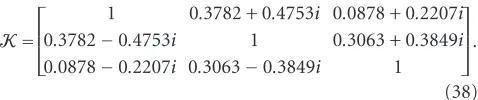
From (3), (20), and (21), we have thedesiredcovariance matrixKas given below:
K=
1 0.3782 + 0.4753i 0.0878 + 0.2207i
0.3782−0.4753i 1 0.3063 + 0.3849i
0.0878−0.2207i 0.3063−0.3849i 1
.
(38)
It is easy to check thatK in (38) is positive definite. Using the proposed algorithm inSection 5, we have the simulation result presented inFigure 4a.
Next, we simulate N = 3 spatially-correlated Rayleigh fading envelopes. We consider an antenna array comprising three transmitter antennas, which are equally separated by a distanceD. Assume thatD/λ=1, that is,D =33.3 cm for GSM 900. Additionally, we assume that ∆ = π/18 rad (or
∆ = 10◦) andΦ = 0 rad. The parametersM,σ2
gj,σ
2 orig,Fs, andFm are the same as in the previous case. From (4), (5), (6), (20), and (21), we have the followingdesiredcovariance matrix:
K=
1 0.8123 0.3730 0.8123 1 0.8123 0.3730 0.8123 1
. (39)
Since Φ =0 rad, the covariancesRxy k,j andRyxk,j between the real and imaginary components of any pair of the com-plex Gaussian random processes (with Rayleigh fading en-velopes) are zeros, and consequently, K is a real matrix. Readers may refer to (5) and (6) for more details. It is easy to realize thatKin (39) is positive definite. The simulation result is presented inFigure 4b.
In Figure 5a, we simulate N = 3 frequency-correlated Rayleigh envelopes based on IEEE 802.11a (OFDM) speci-fications [17]. In particular, the parameters considered here include M = 220, σ
g2j = 1 (j = 1,. . ., 3), σorig2 = 1/2,
Fs = 20 MHz,Fm =555.56 Hz (corresponding to a carrier frequency 5 GHz and a mobile speedv=120 km/h),∆f = 312.5 kHz,στ=0.1 microsecond,τ1,2=τ2,3=1 millisecond,
and τ1,3 = 2 milliseconds. In Figure 5b, we simulate the
case where the covariance matrix is not positive semidefi-nite as mentioned earlier inExample 1ofSection 4.1. From
Figure 5b, we can realize that the three Rayleigh envelopes are highly correlated as we expect (see (11)).
1000
Figure 4: Examples of three equal power-correlated Rayleigh fading envelopes with GSM specifications. (a) Spectral correlation, GSM
specifications. (b) Spatial correlation, GSM specifications.
15
Figure5: Examples of three equal power-correlated Rayleigh fading envelopes with IEEE 802.11a (OFDM) specifications, and with a not
positive semidefinite covariance matrix. (a) Spectral correlation, OFDM specifications. (b) Spatial correlation,Kis not positive semidefinite.
fading envelope by solid curves. In this figure, the param-eter σ2
gj of the PDF is the variance of the complex Gaus-sian random process corresponding to the considered typical Rayleigh fading envelope. It can be observed fromFigure 6
that, the resultant envelopes produced by our algorithm in
the four examples follow accurately the theoretical PDF of the typical Rayleigh fading envelope.
3 2
1 2−1/2.σgj 0
Envelope 0
0.2 0.4 0.6 0.8 1
o
f
R
ay
leig
h
en
velop
es
0.8577/σgj
3 2
1 2−1/2.σgj 0
Envelope 0
0.2 0.4 0.6 0.8 1
o
f
R
ay
leig
h
en
velop
es
0.8577/σgj
3 2
1 2−1/2.σgj 0
Envelope 0
0.2 0.4 0.6 0.8 1
o
f
R
ay
leig
h
en
velop
es
0.8577/σgj
3 2
1 2−1/2.σgj 0
Envelope 0
0.2 0.4 0.6 0.8 1
o
f
R
ay
leig
h
en
velop
es
0.8577/σgj
Figure6: Histograms of Rayleigh fading envelopes produced by the proposed algorithm in the four examples along with a Rayleigh PDF
whereσg2j=1.
algorithms to simulateN=2, 4, 8, 16, 32, 64 or 128 Rayleigh envelopes in a real-time scenario over 10 000 trials. It can be realized fromFigure 7that, forN =64 andN =128, our algorithm is slightly more complex, while it is almost as com-putationally efficient as the method in [2] for a smallerN.
7. CONCLUSIONS
In this paper, we have derived a more generalized algorithm to generate correlated Rayleigh fading envelopes. Using the presented algorithm, one can generate an arbitrary number
N of eitherRayleigh envelopes with any desired powerσ2
rj,
j = 1,. . .,N,or those envelopes corresponding to any de-sired powerσ2
gjof Gaussian random variables. This algorithm also facilitates to generate equal as well as unequal power Rayleigh envelopes. It is applicable to both scenarios of spa-tial correlationandspectral correlationbetween the random processes. The coloring matrix is determined by a positive semidefiniteness forcing procedure and an eigen
decomposi-tion procedure without using Cholesky decomposidecomposi-tion. Con-sequently, the restriction on the positive definiteness of the covariance matrix is relaxed and the algorithm works well without being impeded by the roundoff errors of Matlab. The proposed algorithm can be used to generate Rayleigh envelopes corresponding to any desired covariance matrix, no matter whether or not it is positive definite. In compari-son with the conventional methods, besides beingmore gen-eralized, our proposed algorithm (with or without Doppler spectrum spread) ismore precise, while overcoming all short-comings of the conventional methods.
ACKNOWLEDGMENTS
7 6 5 4 3 2 1
log2N
N=128
N=64 N=32 N=16 N=8 N=4 N=2 0
1 2 3 4 5 6
Ti
m
e
(s
)
Method in [2] Proposed method
Figure7: Computational effort comparison between the method in
[2] and the proposed algorithm.
International Symposium on a World of Wireless, Mobile and Multimedia Networks (IEEE WOWMOM), June 2005.
REFERENCES
[1] D. Verdin and T. C. Tozer, “Generating a fading process for the simulation of land-mobile radio communications,” Electron-ics Letters, vol. 29, no. 23, pp. 2011–2012, 1993.
[2] S. Sorooshyari and D. G. Daut, “Generation of correlated Rayleigh fading envelopes for accurate performance analysis of diversity systems,” inProc. 14th IEEE International Sympo-sium on Personal, Indoor and Mobile Radio Communications (PIMRC ’03), vol. 2, pp. 1800–1804, Beijing, China, Septem-ber 2003.
[3] J. Salz and J. H. Winters, “Effect of fading correlation on adap-tive arrays in digital mobile radio,”IEEE Trans. Veh. Technol., vol. 43, no. 4, pp. 1049–1057, 1994.
[4] R. B. Ertel and J. H. Reed, “Generation of two equal power correlated Rayleigh fading envelopes,”IEEE Commun. Lett., vol. 2, no. 10, pp. 276–278, 1998.
[5] N. C. Beaulieu, “Generation of correlated Rayleigh fading en-velopes,”IEEE Commun. Lett., vol. 3, no. 6, pp. 172–174, 1999. [6] N. C. Beaulieu and M. L. Merani, “Efficient simulation of cor-related diversity channels,” inProc. IEEE Conference on Wire-less Communications and Networking (WCNC ’00), vol. 1, pp. 207–210, Chicago, Ill, USA, September 2000.
[7] H. Adeli and R. Soegiarso,High-Performance Computing in Structural Engineering, CRC Press, Boca Raton, Fla, USA, 1999.
[8] B. Natarajan, C. R. Nassar, and V. Chandrasekhar, “Genera-tion of correlated Rayleigh fading envelopes for spread spec-trum applications,”IEEE Commun. Lett., vol. 4, no. 1, pp. 9– 11, 2000.
[9] W. C. Jakes,Microwave Mobile Communications, John Wiley & Sons, New York, NY, USA, 1974.
[10] D. J. Young and N. C. Beaulieu, “The generation of correlated Rayleigh random variates by inverse discrete Fourier trans-form,”IEEE Trans. Commun., vol. 48, no. 7, pp. 1114–1127, 2000.
[11] T. S. Rappaport, Wireless Communications: Principles and Practice, Prentice Hall PTR, Upper Saddle River, NJ, USA, 2nd edition, 2002.
[12] J. G. Proakis,Digital Communications, McGraw-Hill, Boston, Mass, USA, 4th edition, 2001.
[13] M. J. Gans, “A power spectral theory of propagation in the mobile radio environment,”IEEE Trans. Veh. Technol., vol. VT-21, no. 1, pp. 27–38, 1972.
[14] R. H. Clarke, “A statistical theory of mobile-radio reception,” Bell System Technical Journal, vol. 47, no. 6, pp. 957–1000, 1968.
[15] J. I. Smith, “A computer generated multipath fading simula-tion for mobile radio,”IEEE Trans. Veh. Technol., vol. VT-24, no. 3, pp. 39–40, 1975.
[16] D. J. Young and N. C. Beaulieu, “On the generation of cor-related Rayleigh random variates by inverse discrete Fourier transform,” inProc. 5th IEEE International Conference on Uni-versal Personal Communications (ICUPC ’96), vol. 1, pp. 231– 235, Cambridge, Mass, USA, September–October 1996. [17] IEEE Standards Association, “Part 11: Wireless LAN
medium access control (MAC) and physical layer (PHY) specifications—High-speed physical layer in the 5 GHz band,” 1999, IEEE Standards Association [Online]. available: http://standards.ieee.org/getieee802/.
Le Chung Tran received the excellent B. Eng. degree with the highest distinction and the M. Eng. degree with the highest dis-tinction in telecommunications engineer-ing from Hanoi University of Communi-cations and Transport and Hanoi Univer-sity of Technology, Vietnam, in 1997 and 2000, respectively. From March 2002 to July 2005, he worked towards the Ph.D. degree in telecommunications engineering at the
School of Electrical, Computer and Telecommunications Engineer-ing, University of Wollongong, Australia. He is currently working as an Associate Research Fellow at the Telecommunications and In-formation Technology Research Institute (TITR), School of Elec-trical, Computer and Telecommunications Engineering, Univer-sity of Wollongong, Australia. He has been working as a Lecturer at Hanoi University of Communications and Transport, Vietnam, since September 1997 to date. He has achieved numerous national and overseas awards, including World University Services (WUS) (twice), Vietnamese Government’s Scholarship, Wollongong Uni-versity Postgraduate Award (UPA), Wollongong UniUni-versity Tuition Fee Waver, during the undergraduate and postgraduate periods. His research interests include transmission diversity techniques, mobile communications, space-time processing, MIMO systems, channel propagation modelling, ultra-wideband communications, OFDM, and spread-spectrum techniques. He is a Member of IEEE.
Tadeusz A. Wysockireceived the M.S.Eng. degree with the highest distinction in telecommunications from the Academy of Technology and Agriculture, Bydgoszcz, Poland, in 1981. In 1984, he received his Ph.D. degree, and in 1990, was awarded a D.S. degree (habilitation) in telecommuni-cations from the Warsaw University of Tech-nology. In 1992, he moved to Perth, Western Australia, to work at Edith Cowan
Fellowship. After returning to Australia, he was appointed a Pro-gram Leader, Wireless Systems, within Cooperative Research Cen-tre for Broadband Telecommunications and Networking. Since De-cember 1998, he has been working as an Associate Professor at the University of Wollongong, NSW, within the School of Electrical, Computer and Telecommunications Engineering. The main areas of his research interests include indoor propagation of microwaves, code division multiple access (CDMA), and digital modulation and coding schemes. He is the author or coauthor of four books, over 100 research publications, and nine patents. He is a Senior Member of IEEE.
Alfred Mertinsreceived his Dipl.-Ing. de-gree from the University of Paderborn, Ger-many, in 1984, the Dr.-Ing. degree in electri-cal engineering and the Dr.-Ing. Habil. de-gree in telecommunications from the Ham-burg University of Technology, Germany, in 1991 and 1994, respectively. From 1986 to 1991 he was with the Hamburg Uni-versity of Technology, Germany, from 1991 to 1995 with the Microelectronics
Applica-tions Center, Hamburg, Germany, from 1996 to 1997 with the Uni-versity of Kiel, Germany, from 1997 to 1998 with the UniUni-versity of Western Australia, and from 1998 to 2003 with the University of Wollongong, Australia. In April 2003, he joined the University of Oldenburg, Germany, where he is a Professor in the Faculty of Mathematics and Science. His research interests include speech, au-dio, image and video processing, wavelets and filter banks, and dig-ital communications. He is a Senior Member of IEEE.
Jennifer Seberryreceived the Ph.D. degree in computation mathematics from La Trobe University in 1971. She has subsequently held positions at the Australian National University, The University of Sydney and ADFA, The University of New South Wales. She has published extensively in discrete mathematics and is world renown for her new discoveries on Hadamard matrices and statistical designs. In 1970 she cofounded