R E S E A R C H
Open Access
Channel estimation for FDD massive
MIMO system by exploiting the sparse
structures in angular domain
Yurong Wang
1, Xiaochen Xia
1,2*, Kui Xu
1, Wei Xie
1and Minghai Wang
2Abstract
Massive multiple-input multiple-output (MIMO) is a powerful supporting technology to meet the energy/spectral efficiency and reliability requirement of Internet of Things (IoT) network. However, the gain of massive MIMO relies on the availability of channel state information (CSI). In this paper, we investigate the channel estimation problem for frequency division duplex (FDD) massive MIMO system. By analyzing the sparse property of the downlink massive MIMO channel in the angular domain, a structured prior-based sparse Bayesian learning (SP-SBL) approach is proposed to estimate the downlink channels between base station (BS) and users reliably. The scheme can be implemented without the knowledge of channel statistics and angular information of users. The simulation results show that the proposed scheme outperforms the reference schemes significantly in terms of normalized mean square error (NMSE) for a variety of scenarios with different lengths of pilot sequence, transmit signal-to-noise ratios (SNRs), and angular spreads.
Keywords: FDD massive MIMO, Channel estimation, Structured prior, Sparse Bayesian learning, Normalized mean square error
1 Introduction
As an emerging technology that aims to allow everything to connect, interact, and exchange data, the Internet of Things (IoT) has attracted extensive attention in vari-ous areas such as governments, industry, and academia [1]. The massive connectivity, strict energy limitation, and requirement of ultra-reliable transmission are often termed as the most distinct features of IoT [2, 3]. These features make massive multiple-input multiple-output (MIMO) [4] a natural supporting technology for IoT since through coherent processing over the signals of large-scale antenna array, massive MIMO can produce tremendous spectral/energy efficiency gain and improve the reliability of IoT transmission significantly.
However, the coherent processing depends on the reliable estimation of channel state information (CSI) between base station (BS) and users [5–7]. In time division
*Correspondence:[email protected]
1Institute of Communication Engineering, Army Engineering University of PLA, No. 88, Houbiaoying Street, Nanjing 0086-210007, China
231682 Army of PLA, Lanzhou, China
duplex (TDD) massive MIMO system, by exploiting the channel reciprocity, both the uplink and downlink chan-nels can be obtained using the simple least square (LS) approach [8]. The consumption of pilot resource scales with the number of users. However, there is no channel reciprocity in frequency division duplex (FDD) massive MIMO system. In this case, the downlink channel estima-tion becomes particularly challenging since the downlink training and corresponding CSI feedback yield an unac-ceptably high overhead. For example, with the traditional LS channel estimation scheme, it is well-known that the length of the required pilot sequence must be larger than the number of antennas at BS [8], which will degrade the system performance greatly.
In the practical system, the BS is usually elevated at a relatively high altitude with few surrounding scatters. Therefore, the scattering process often occurs in vicinity of user, which results in very narrow signal angle of depar-ture (AoD) at BS [8, 9] for far-field transmission. Based on a physical channel model, several works have shown that the signals from different antennas of BS exhibit high correlation, and hence, the channel between BS and user
can be represented by a sparse vector in some alternate domain (usually called angular domain) [10, 11]. This property can be utilized to design cost-efficient chan-nel estimation schemes [12–14]. The main idea behind is to transform the channel to the angular domain by exploiting the correlations between the channel elements and then estimate the effective low-dimension angular-domain channel with the LS or minimum mean square error (MMSE) method. In this way, the training con-sumption can be reduced greatly. However, these schemes require the knowledge of channel covariance matrix or angular-domain information, such as the AoDs of the sig-nals, which is not always available. Another path to reduce the training overhead is to formulate the channel esti-mation as a sparse recovery problem and estimate the angular-domain channel using the algorithms in compres-sive sensing, such as orthogonal matching pursuit (OMP) [15, 16] and sparse Bayesian learning (SBL) [17]. These schemes do not need the channel covariance matrix and angular information; however, suffer from performance loss when the length of pilot sequence is small. To improve the quality of channel estimation, novel channel esti-mation schemes based on block l1/l2 optimization [18] and variational SBL [19] were proposed recently. These schemes exploit the structures in the channel sparsity to give a robust channel estimation.
In this paper, we investigate the downlink channel esti-mation problem for FDD massive MIMO system consid-ering the above challenges. The main contributions are as follows:
1 The sparse property of downlink massive MIMO channel in angular domain is analyzed theoretically. The results show that the angular-domain channel exhibits two kinds of sparse structures, namely the joint sparsity and burst sparsity.
2 By exploiting the two kinds of sparsity, a structured prior-based SBL (SP-SBL) approach is proposed to estimate the downlink channel between the BS and user reliably. The scheme does not require the channel statistics and AoD information.
3 Extensive numerical simulations are presented to validate the effectiveness of the proposed scheme. The results show that the proposed scheme outperforms the reference schemes significantly in terms of normalized mean square error (NMSE) for a variety of scenarios with different lengths of pilot sequence, transmit signal-to-noise ratios (SNRs), and angular spreads.
Notations: We useB∗,BT, BH,|B|, andBto denote conjugate, transpose, conjugate transpose, determinant, and Frobenius norm of matrixB, respectively.B∈CN×M
meansBis anN×Mcomplex-valued matrix.CN(b|m,C)
means thatbis a complex Gaussian variable with mean
mand covariance matrixC. [B]i,jdenotes thei,jth ele-ment of matrixB.E(·)denotes the expectation.∇b
f(b)
denotes the gradient of functionf(b)w.r.t. the vectorb.
2 Methods
The rest of the paper is organized as follows: Section 3 describes the system model of the FDD massive MIMO system. Section 4 analyzes the sparse property of the angular-domain channel and presents the SP-SBL-based channel estimation scheme. Section5presents the simu-lation results to validate the effectiveness of the proposed scheme. Section6draws the conclusions.
3 System model
Consider the massive MIMO system with a BS and K
users. It is assumed that both the BS and users are equipped with uniform linear arrays (ULAs) with half wavelength antenna spacing. The numbers of antennas at BS and user areNandM, respectively, which satisfyM N. According to the ray-tracing model [8], the downlink channel between BS and userkcan be expressed as:
Hk = denotes the angle of arrival (AoA) w.r.t. the array of user
k.dandadenote the corresponding angular spreads. rk(θ,ϕ)denotes the complex channel gain for angle{θ,ϕ}.
aBS(θ)andaU(ϕ)denote the array steering vectors, which are given by:
In practice, the BS is often deployed at a high place such as the top of high building. As discussed in the introduc-tion, the limited number of scatterers around BS will result in very narrow angular spreaddin far-field propagation. Conversely, the waves arriving at the user are usually uni-formly distributed in AoA. Therefore, it is reasonable to assumeais close toπ[9]. Note that the proposed chan-nel estimation scheme in the next section is very general, which is valid for arbitrarya.
Let S denote the N × T pilot matrix of BS which is broadcasted inT successive symbol times. The power of each pilot symbol is|[S]i,j|2= P. For a practical training scheme,T should be much smaller thanN. The received training signal at userkcan be expressed as:
where N ∈ CM×T denotes the additive white Gaussian noise (AWGN) matrix whose elements have zero mean and varianceσ2.
Note that for the full-duplex massive MIMO system with separate antenna configuration [11], the channel reciprocity is also not available which makes the downlink channel estimation very challenging. Since the downlink transmission model of full-duplex massive MIMO is sim-ilar with the FDD counterpart in the above, the proposed scheme can be utilized to estimate the downlink channel directly to reduce the pilot consumption.
4 Channel estimation by exploiting the sparse
structures
In this section, we first analyze the property of channel sparsity in the angular domain. Based on the theoretical results, we propose a novel SP-SBL approach to estimate the downlink channel between BS and user.
4.1 Joint and burst sparsity in the angular domain
According to [11], the angular-domain channel matrix between BS and userkcan be expressed as:
Xk=AHNHk ∈CN×M (4)
whereAN is a shifted discrete Fourier transform (DFT) matrix of dimensionN, that is:
AN = aN the angular-domain channel vector between the BS and themth antenna of userk. The angular-domain channel is the projection of channel onto the space spanned by the DFT bases. Since a DFT basis is in fact equivalent to an array steering vector with specific AoD, the angular-domain channel can be viewed as the channel response in the angular domain, and the amplitude of each angular-domain channel element indicates the channel strength for the path with specific AoD. Moreover, due to the lim-ited number of scatterers around the BS, the spread of AoD will be very narrow in far-field propagation scenario. As a result, only a small fraction of elements in angular-domain channel matrix has significant amplitude. This results in the sparsity in angular-domain channel.
Mathematically, following a similar analytic approach as that in [10, 11], it can be shown that the angular-domain channel matrix has the following two kinds of sparse structures.
• Joint sparsity among the columns ofXk: Thenth element ofxk,mhas a significant amplitude only when
n∈ k, where kis given by k = indexm, the indexes of the significant elements in each column ofXkare the same.
• Burst sparsity in each column ofXk: The indexes of significant elements inxk,mappear in block.
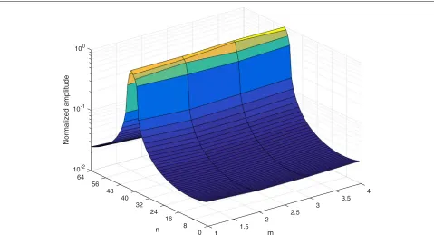
As discussed in the above,dis commonly small. Thus, only a small number of elements in xk,m has a signifi-cant value. Physically, the joint sparsity of angular-domain channel is due to the fact that the size of the user’s array can be neglected in far-field propagation, and thus, the channels between the BS and all antennas of user can be considered to have similar property in the angular domain. Moreover, it is noted that the AoD of downink signal varies in a continuous interval [θk−d,θk+d]. This causes the burst sparsity nature in the angular-domain channel. The two kinds of sparse structures are shown in Fig.1for an example withN=64 andM=4.
Here, we shall point out that, for the practical system with finite N, the nth element of xk,m with n ∈/ k is small but not zero as shown in Fig.1. Therefore,xk,m is in fact approximately sparse. Note that [16,18] assumed that the angular-domain channel element is exactly zero if
n∈/ k, which we call as exactly sparse channel. Although this assumption simplifies the model, it may change the real system performance in the high SNR region greatly as will be shown in the simulation of Section5.
4.2 Structured prior-based Bayesian channel estimation
By substituting (4) in (3), the received training signal at userkcan be rewritten as:
Yk=ZHk =Xk+NTk ∈CT×M (6) where = SHAN ∈ CT×N. Note that as long asXk is known, the channel matrixHk can be recovered directly based on (4), that is, Hk = AXk (which is called basis expansion model).
By treatingas the sensing matrix,Xkcan be estimated using the conventional SBL [17] or OMP [15] approach from (6). However, the performance will be poor if the number of pilot symbols (i.e.,T) is small as will be seen in the simulations. In this paper, we propose a SP-SBL approach to estimate the channel reliably by exploiting the two kinds of sparse structures discussed in the last subsection.
10-2
Fig. 1Normalized amplitudes for the elements of angular-domain channel matrixXk, whereN=64,M=4, andθk=15.5◦. The angular spread for
AoD isδd=5◦. It is assumed that the waves arriving at the user are usually uniformly distributed in AoA [12]. Therefore,ais equal toπ
whereγk =
DkanN×Ndiagonal matrix whosenth diagonal element is modeled as: angular-domain channel matrixXk has precision matrix
γk,mDk. Thus, precision matrices for different columns of
Xk differ only with a scaling factor γk,m. This property captures the joint sparsity among the columns ofXk. The parameterγk,mis utilized to model the relative difference between the amplitudes ofxk,m
M
m=1. By exploiting the joint sparsity, the recovery errors which predict zero for one element ofxk,mand predict non-zero for the element ofxk,m (m = m) in the same position can be mitigated effectively.
Additionally, the precision of thenth element of xk,m can be expressed asγk,m
αk,n−1+αk,n+αk,n+1
. Thus, the precisions of adjacent elements inxk,mare mutually coupled. When αk,n → ∞, the estimations of nth, (n − 1)th, and (n + 1)th elements of xk,m will be driven to zero simultaneously. Therefore, the zero elements (and hence non-zero elements) in the estimation ofxk,m will appear in block, which just captures the block sparsity structure.
By exploiting burst sparsity, the situation that a signifi-cant element ofxk,m is predicted as zero (or near zero), isolated in xk,m, can be reduced greatly. Note that the precisions of the first and the last elements of xk,m are also coupled. This structure captures a basic property of angular-domain channel, i.e., the elements at the begin-ning and that at the end ofxk,mtend to be close to zero or have large amplitude simultaneously.
According to (6), the likelihood function of the received training signalYkcan be expressed as:
p(Yk|Xk)= distribution, the posterior distribution of xk,m can be derived as:
To give a fully Bayesian treatment, similar to conven-tional SBL, we introduce a gamma hyperprior for αk:
p(αk)=
whereaandbare fixed parameters. Commonly,aandb
are set as small values to impose a non-informative prior. In this paper, a and b are chosen as a = b = 10−4. Moreover, we introduce a Dirichlet hyperprior forγk:
p(γk)=C(u) stant. Since the expectation ofγk,m with respect to the distribution (13) is given byEγk,m= um
u0, we can
inter-pretuas the parameter which gives an initial guess on the relative difference between the amplitudes ofxk,m
M
m=1. As in the convention of sparse Bayesian learning frame-work, the hyperpriors are utilized to imbed the prior knowledge of the parameters into the estimation algo-rithm. Moreover, as shown in [17], the utilization of gamma hyperprior is helpful to produce a sparse solution which is desired in our problem.
As long asαkandγkare obtained, the maximum poste-rior (MAP) estimation ofXkcan be given by its posterior mean in (11). Therefore, in the following, we focus on finding the optimalαk andγkby solving the MAP prob-lem:
Different from the conventional SBL, solving the above problem directly is quite challenging due to the utilization of the structured prior. To address this problem, we resort to the expectation maximization (EM) [20] algorithm to find a computationally efficient solution.
4.3 Solving the SP-SBL using expectation maximization
Instead of solving the MAP problem in (14) directly, the EM algorithm tries to find the optimal αk and γk by maximizing the expected complete-data log-likelihood function, that is:
where the expectation is w.r.t. the posterior distribution ofXk given by (10).αˆkoldandγˆkolddenote the latest esti-mations of αk andγk, respectively. Each iteration of the algorithm consists of an expectation step (E-step) and a maximization step (M-step).
In the E-step of the ith iteration, the posterior dis-tribution of Xk is computed approximately using the estimations of αk and γk in the (i − 1)th iteration
denoted byαˆ(ki−1)andγˆk(i−1) based on (10), which is then used to evaluate the expected complete-data log-likelihood function.
In the M-step of theith iteration, the estimation ofαk andγk is updated to maximize the expected complete-data log-likelihood function obtained in E-step.
4.3.1 Update ofγk
By substituting (10) and (13) into (15) and discarding the terms irrelevant toγk, it can be shown that the expected complete-data log-likelihood function reduces to"
Qαˆk(i−1),γk
Note that αk has been fixed at its estimation after the last iteration, i.e., αk = αˆk(i−1) . Dˆk can be
. The first-order derivative of
Qαˆ(ki−1),γk
By setting (17) to zero, we can obtain the estimation for
Q
where γk has been fixed at its estimation after the last iteration, i.e., γk = ˆγk(i−1). The first-order derivative of solution forαk,nunavailable. Nevertheless, we can obtain a valid solution using the gradient-based algorithm as follows:
where δis the stepsize, and the gradient can be directly computed using (20).
By virtue of the EM’s properties, the above algorithm will always converge since each iteration is guaranteed to reduce the target function. However, the update formula of αk in (22) is still complex due to the lack of analytic expressions. Moreover, (22) gives little insight into the basic mechanism of SP-SBL. In the following, we derive a closed-form solution for αk by adding some heuristic assumptions.
When updating αk,n, we temporarily assume that the nth element ofxk,mhas the same variance with its neigh-bors, i.e., the (n−1)th and(n+1)th elements ofxk,m. In this case, we will have αk,n−2 = αk,n−1 = αk,n =
αk,n+1 = αk,n+2. This assumption is reasonable if we do not have much prior knowledge aboutαk. Note that this does not mean we will obtain an estimation of αk with
ˆ the incoming training signal, the estimation ofαk,nis rec-tified and is expected to get close to the true value. Under this assumption, (20) becomes:
dQαk,γˆk(i−1)
The numerical results show that the update formula in (24) gives rise to the similar performance with that using gradient-based update in (22). Moreover, the solution in (24) provides a clear insight into the difference between SP-SBL and conventional SBL. With conventional SBL, the update of the precision for thenth element ofxk,mis only related to the posterior mean and variance of itself. In contrast, in SP-SBL, the update of αk,n is effected by the posterior means and variances of(n−1)th,nth, and
(n+1)th elements ofxk,m for allm = 1,· · ·,Mdue to the utilization of joint and burst sparsity. Therefore, the SP-SBL is expected to achieve better performance.
After the downlink channel estimation, the estimated CSI should be sent back to the BS in order to perform the downlink beamforming. In this process, additional error can be introduced by quantization, noise, and feedback delay. However, the results in [21] showed that the error due to the imperfect feedback can be made much smaller than that due to the estimation error in downlink training phase. Therefore, as in [11], we optimistically neglect the additional error due to the feedback in this paper.
4.4 Computation complexity analysis
The main computation load in each iteration is due to
the N × N matrix inversion when updating the
poste-rior mean and covariance matrix of xk,m in E-step. By using the matrix inversion lemma, the calculation of each matrix inversion has complexity OT3. Therefore, the overall computational complexity of the algorithm scales
with OGKMT3, where G is the number of EM
iter-ations. Since we consider the situation that T is much smaller thanN, the computation complexity will not pose a significant problem.
4.5 Extension to FDD massive MIMO system with hybrid analog-digital processing
In the practical system, the hybrid analog-digital process-ing may be utilized at the BS to reduce the implementation complexity. In the following, we will show that the pro-posed scheme can still be applied in this case. With hybrid analog-digital processing at the BS, the received training signal at userkcan be expressed as:
whereW ∈ CN×F is the arbitrary analog beamforming matrix utilized by BS, andF ≤ Ndenotes the number of radio frequency chain at the BS. The pilot signalSis an
F×T matrix in this case. Note that we have reuse some notations to avoid introducing too many new definitions. Using the definition of angular-domain channel in (4), we can rewrite (25) as:
Yk=ZHk =(WS)HANXk+NTk (26) Note that, by treating(WS)HAN as the sensing matrix, (26) is in the same form with (6). Therefore, the proposed scheme can be utilized directly to estimation the channel matrix from (26).
5 Simulation results and discussion
This section presents the simulation results to validate the proposed scheme. Without loss of the generality, the large-scale fading and noise variance are normal-ized to 1. For illustration, the number of users is set
to K = 8. The central frequency is set to 2.4 GHz,
and the antenna spacing is equal to the half of wave-length. Similar to [22], the rows of sensing matrix are designed as the length-N Zadoff-Chu sequence [23] with shifting step 7. In particular, the first row of is given by √1
N 1,e
jνπN12,ejνπN22,· · ·,ejνπ(NN−1)2
. The
sec-ond row of is obtained by cyclically right
shift-ing the first row with a step of 7, which is given
by √1 tions. The rest rows ofare generated in a similar way. The AoDθkand AoAϕk for different users are generated randomly from the interval [−90◦, 90◦]. It is assumed that the waves arriving at the user are uniformly distributed in AoA [12]. Therefore,a is equal toπ, and the complex channel gain reduces tork(θ,ϕ) = rk(θ). It is assumed that therk(θ)for differentθ are uncorrelated. For each sample of θ, rk(θ) is the complex Gaussian distributed with zero mean and varianceUk(θ), whereUk(θ)is the power angle spectrum. We modelUk(θ)as the truncated Laplacian distribution centered atθk [12]. The simplified update rule forαk in (24) is utilized to reduce the com-plexity. The parameters in the hyperprior models (12) and (13) are set asa=b=10−4,u1= · · · =uM, andu0=M. We consider four reference schemes in the simulations, i.e., the conventional SBL based on the original algorithm in [17], OMP [15], block l1/l2 minimization [18], and variational SBL [19]. Note that the blockl1/l2 minimiza-tion and variaminimiza-tional SBL can also exploit the joint sparsity among the angular-domain channel vectors between BS and different antennas of user.
We consider the NMSE performance which is defined as follows:
All figures are obtained by averaging the results for 103 independent channel realizations.
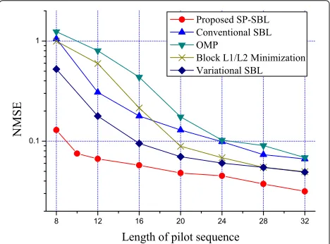
Figure 2 shows the NMSE performance for different
lengths of pilot sequenceT, where the transmit SNR of BS is NPσ2 = 15 dB and the angular spread isd = 5◦. It is seen that the performances of conventional SBL and OMP are poor when the length of pilot sequence is small. By exploiting the joint sparsity among the angular-domain channel vectors between BS and different antennas of user, the block l1/l2 minimization and variational SBL can provide better performance. Moreover, the proposed scheme based on SP-SBL achieves the best NMSE perfor-mance since it exploits the joint sparsity and burst sparsity simultaneously.
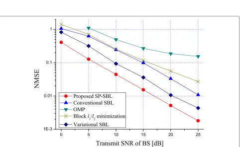
Figure 3 shows the NMSE performance for different
transmit SNRs of BS, where the length of pilot sequence isT = 16 and the angular spread isd = 5◦. It is seen that the performances of all schemes converge to NMSE floors for large SNR. The reason is that the angular-domain channel is approximately sparse as discussed in Section4.1. That is, thenth element ofxk,mwithn∈/ k is small but not zero. With smallT, recovering all these small elements ofxk,m with high accuracy is difficult. As a result, with the increasing of the SNR, the effect of the mismatch between the true values of these small elements and their estimates becomes significant when compared with AWGN, which incurs NMSE floor in the high SNR region1. Note that the NMSE floor does not occur in
Fig. 3NMSE performance for different transmit SNRs of BS, whereN=64 andM=4. The length of pilot sequence isT=16 and the angular spread isd=5◦
Fig. 5Number of significant elements inxk,m, whereN=64 andM=4
Fig. 6NMSE performance for different angular spreadsd, whereN=64 andM=4. The length of pilot sequence isT=16 and the transmit SNR
of BS isNP
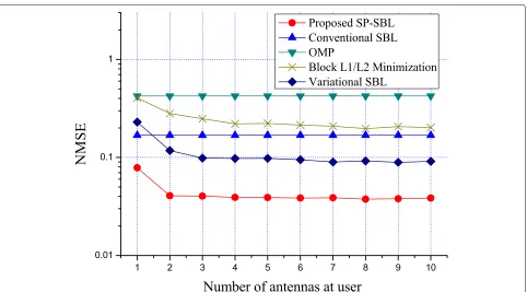
Fig. 7NMSE performance for different numbers of antennas at users, i.e.,M, whereN=64. The length of pilot sequence isT=16. Transmit SNR of BS isNPσ2 =15 dB. The angular spread isd=5◦
Fig. 8NMSE performance for different numbers of iterations, whereN=64. The length of pilot sequence isT=16. Transmit SNR of BS is
NP
the simulations of [16,18]. This is because these works assume that there is no channel power leakage outside k. Although this assumption simplifies the model, the resul-tant simulations cannot reflect the real performance in the high SNR region very well. For illustration, we also present the NMSE performance for all schemes in Fig.4 under exactly sparse angular-domain channel model considered in [16,18], where the nth element ofxk,m is set to zero as long asn ∈/ k when generating the channel matrix. From the figure, we can see that the performance floors disappear as expected.
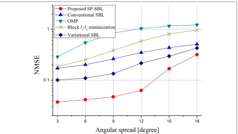
Then, we consider the performance for different angu-lar spreadsd ranged from 3 to 18◦. This corresponds to the scenarios with scattering ring of 30 m and the dis-tance between BS and user varying from about 100 to 500 m. Figure5shows the number of significant elements in the angular-domain channelxk,m, i.e., the number of elements that contain 90% of the channel power, varies from 3 to 17 when the angular spread increases from 3 to 18◦. Figure6shows the NMSE performance for different angular spreads, where the transmit SNR of BS is NPσ2 =
15 dB and the length of pilot sequence isT = 16. Again, the proposed scheme based on SP-SBL achieves the best performance. Moreover, we note that the NMSEs of all schemes degrade when the angular spread increases. This is because the number of significant elements in angular-domain channel becomes larger as shown in Fig.5. In this case, to maintain the estimation performance, the capac-ity of all schemes must be enhanced by increasing the training samples.
Figure 7 shows the NMSE performance for different
numbers of antennas at user, i.e.,M. The length of pilot sequence is T = 16. The transmit SNR of BS is NPσ2 =
15 dB. The angular spread isd = 5◦. It is seen that the NMSEs of conventional SBL and OMP-based schemes are independent ofM. In contrast, the performances of block
l1/l2 minimization, variational SBL, and SP-SBL-based schemes are improved gradually with the increasing ofM, which is just the benefit of exploiting the joint sparsity.
Figure 8 shows the NMSE performance for different
numbers of iterations. The length of pilot sequence is
T = 16. The transmit SNR of BS is NPσ2 = 15 dB. The
angular spread is d = 5◦. It is seen that the NMSE performance converges after 40 EM iterations. More-over, the number of iterations required for SP-SBL is smaller than that of blockl1/l2minimization and greater than that of conventional SBL and variational SBL. The computation complexities in each iteration for SP-SBL, block l1/l2 minimization, conventional SBL, and varia-tional SBL are OKMT3, O(KMNT) [18], OKMT3
[17], andOKMT3[19], respectively. Note that the OMP needs no iteration and its total computation complexity is O(ηKMNT)[15], whereηdenotes the number of signifi-cant elements inxk,m. Therefore, from the analysis above,
the SP-SBL has the highest computation complexity but converges to best NMSE.
6 Conclusions
This paper proposes a SP-SBL approach for downlink channel estimation in FDD massive MIMO system. By exploiting the two kinds of sparse structures, the scheme can substantially reduce the pilot resource assumption while maintaining the estimation performance. Through numerical simulations, it is shown that the proposed scheme outperforms the reference schemes significantly in terms of NMSE for a variety of scenarios with differ-ent lengths of pilot sequence, transmit SNRs, and angular spreads.
Endnote
1To address this problem, a possible solution is to
exploit other inherent structures of angular-domain chan-nel in the prior model, for example, the additional correla-tion between the phases and amplitudes of the elements in angular-domain matrix if they exist. In general, the prob-lem is quite challenging and will be considered as future study.
Abbreviations
AoA: Angle of arrival; AoD: Angle of departure; AWGN: Additive white Gaussian noise; BS: Base station; CSI: Channel state information; DFT: Discrete Fourier transform; EM: Expectation maximization; FDD: Frequency division duplex; IoT: Internet of Things; LS: Least square; MIMO: Multiple-input multiple-output; MMSE: Minimum mean square error; NMSE: Normalized mean square error; OMP: Orthogonal matching pursuit; SBL: Sparse Bayesian learning; SNR: Signal-to-noise ratio; SP-SBL: Structured prior-based sparse Bayesian learning; ULA: Uniform linear array
Funding
This work is supported by National Natural Science Foundation of China (No. 61671472) and Jiangsu Province Natural Science Foundation (BK20160079).
Availability of data and materials
Not applicable.
Authors’ contributions
XX provided the main idea and is responsible for the manuscript writing. YW conducted the simulations. KX, WX, and MW assisted with the revision of the manuscript. All authors have read and approved the final manuscript.
Competing interests
The authors declare that they have no competing interests.
Publisher’s Note
Springer Nature remains neutral with regard to jurisdictional claims in published maps and institutional affiliations.
Received: 4 December 2018 Accepted: 18 January 2019
References
1. J. A. Stankovic, Research directions for the Internet of Things. IEEE Internet Things J.1(1), 3-9 (2014)
3. C. Li, S. Zhang, P. Liu, F. Sun, J. M. Cioffi, L. Yang, Overhearing protocol design exploiting intercell interference in cooperative green networks. IEEE Trans. Veh. Technol.65(1), 441-446 (2016)
4. T. L. Marzetta, Noncooperative cellular wireless with unlimited numbers of base station antennas. IEEE Trans. Wirel. Commun.9(11), 3590–3600 (2010)
5. C. Li, L. Yang, W. Zhu, Two-way, MIMO relay precoder design with channel state information. IEEE Trans. Commun.58(12), 3358–3363 (2010) 6. C. Li, H. J. Yang, F. Sun, J. M. Cioffi, L. Yang, Multiuser overhearing for
cooperative two-way multiantenna relays. IEEE Trans. Veh. Technol.65(5), 3796–3802 (2016)
7. C. Li, P. Liu, C. Zou, F. Sun, J. M. Cioffi, L. Yang, Spectral-efficient cellular communications with coexistent one- and two-hop transmissions. IEEE Trans. Veh. Technol.65(8), 6765–6772 (2016)
8. A. Adhikary, J. Nam, J.-Y. Ahn, G. Caire, Joint spatial division and multiplexing: the large-scale array regime. IEEE Trans. Info. Theory.59(10), 6441–6463 (2013)
9. C. Sun, X. Gao, S. Jin, M. Matthaiou, Z. Ding, C. Xiao, Beam division multiple access transmission for massive MIMO communications. IEEE Trans. Commun.63(6), 2170–2184 (2015)
10. H. Xie, F. Gao, S. Zhang, S. Jin, A unified transmission strategy for TDD/FDD massive MIMO systems with spatial basis expansion model. IEEE Trans. Veh. Technol.66(4), 3170–3184 (2017)
11. X. Xia, K. Xu, D. Zhang, Y. Xu, Y. Wang, Beam-domain full-duplex massive MIMO: realizing co-time co-frequency uplink and downlink transmission in the cellular system. IEEE Trans. Veh. Technol.66(10), 8845–8862 (2017) 12. L. You, X. Gao, X. Xia, N. Ma, Y. Peng, Pilot reuse for massive MIMO
transmission over spatially correlated rayleigh fading channels. IEEE Trans. Wireless Commun.14(6), 3352–3366 (2015)
13. L. You, X. Gao, A. L. Swindlehurst, W. Zhong, Channel acquisition for massive MIMO-OFDM with adjustable phase shift pilots. IEEE Trans. Signal Process.64(6), 1461–1476 (2016)
14. L. Zhao, D. W. K. Ng, J. Yuan, Multi-user precoding and channel estimation for hybrid millimeter wave systems. IEEE J. Sel. Areas Commun.35(7), 1576–1590 (2017)
15. J. Lee, G. T. Gil, Y. H. Lee, Channel estimation via orthogonal matching pursuit for hybrid MIMO systems in millimeter wave communications. IEEE Trans. Commun.64(6), 2370–2386 (2016)
16. X. Rao, V. K. N. Lau, Distributed compressive CSIT estimation and feedback for FDD multi-user massive MIMO systems. IEEE Trans. Signal Process.
62(12), 3261–3271 (2014)
17. S. Ji, Y. Xue, L. Carin, Bayesian compressive sensing. IEEE Trans. Signal Process.56(6), 2346–2356 (2008)
18. C. C. Tseng, J. Y. Wu, T. S. Lee, Enhanced compressive downlink CSI recovery for FDD massive MIMO systems using weighted block
1-minimization. IEEE Trans. Commun.64(3), 1055–1067 (2016) 19. X. Cheng, J. Sun, S. Li, Channel estimation for FDD multi-user massive
MIMO: a variational Bayesian inference-based approach. IEEE Trans. Wirel. Commun.16(11), 7590–7602 (2017)
20. A. Dempster, Maximum likelihood from incomplete data via the EM algorithm. J. R. Stat. Soc. Ser. B.39(1), 1–38 (1977)
21. G. Caire, N. Jindal, M. Kobayashi, N. Ravindran, Multiuser MIMO achievable rates with downlink training and channel state feedback. IEEE Trans. Inf. Theory.56(6), 2845–2866 (2010)
22. Y. Ding, S. E. Chiu, B. Rao, Bayesian channel estimation algorithms for massive MIMO systems with hybrid analog-digital processing and low-resolution ADCs. IEEE J. Sel. Top. Sig. Process.12(3), 499–513 (2018) 23. D. Chu, Polyphase codes with good periodic correlation properties. IEEE