Online rate adjustment for adaptive random access compressed sensing of time varying fields

R E S E A R C H

Open Access

Online rate adjustment for adaptive

random access compressed sensing of

time-varying fields

Naveen Kumar

, Fatemeh Fazel

, Milica Stojanovic

and Shrikanth S. Naryanan

Abstract

We develop an adaptive sensing framework for tracking time-varying fields using a wireless sensor network. The sensing rate is iteratively adjusted in an online fashion using a scheme that relies on an integrated sensing and communication architecture. As a result, this scheme allows for an implementation that is both energy efficient and robust. The objective is to promote an “active" framework which uses the information extracted from the network data and iteratively adjusts the monitoring process to capture the temporal variations in the monitored field. We propose two metrics based on target detection/tracking for this feedback scheme that seek to trade off between energy efficiency and accuracy of the detection/tracking tasks. Our simulation results suggest that tying target detection with the rate adjustment algorithm ensures that the robustness to changes in the field can be achieved simultaneously with the end goal of accurate target detection. Compared to a baseline method that uses the correlation of the acquired field over time, our method exhibits better performance when the targets of interest have a smaller spatial spread.

Keywords: Sensor networks, Adaptive sensing, Detection, Random access, Compressed sensing, Joint communication and detection

1 Introduction

The emergence of compressed sensing framework presents significant potential for efficient sensing and sampling systems [1–3] by helping to reduce sample complexity under realistic communication constraints. Sensor network technology greatly benefits from the compressed sensing paradigm [4–12]. Consider for exam-ple, large-scale networks that are deployed for long-term monitoring of dynamic fields such as the ocean bed that typically need to account for power consumption con-siderations. An efficient scheme in such cases requires performance optimization that jointly considers both the sensing and communication constraints.

To address this issue, Fazel et al. proposed a random access compressed sensing (RACS) scheme in [13, 14] for energy-efficient reconstruction of sensing fields. The pro-posed sensing scheme depends on integrating information from the communication and channel access modules into

*Correspondence: komathnk@usc.edu

1Signal Analysis and Interpretation Laboratory (SAIL), Electrical Engineering, University of Southern California, Los Angeles, CA, USA

Full list of author information is available at the end of the article

the data acquisition process. The method is simple to implement under realistic communication constraints and requires minimal assumptions on the field. However, the proposed RACS scheme is designed for stationary1 sens-ing fields, where the field besens-ing monitored is assumed to remain static during sensing. In order to monitor time-varying fields, in [15], the authors employed low-rank matrix recovery to reconstruct the space-time map of the field. However, this approach is offline and entails con-siderable delays since full recovery can be attained only after the data have been collected over multiple time segments. Moreover, it is assumed that the coherence properties of the underlying field are known a priori and remain unchanged throughout the full sensing duration. This assumption might be justified for the monitoring of natural phenomena, where the field is assumed to be either stationary or changing at a fixed rate. It is also com-mon to find similar assumptions of stationarity in related works in object detection or classification in underwater fields [16, 17]. However, when the field being monitored undergoes a varying rate of change (e.g., when the process

is impacted by a target that is moving at an unknown or variable speed), such assumptions may not hold.

In a more recent work, Kerse et al. [18] addressed this problem by proposing to unify target detection with reconstruction using a standard sparse identification tech-nique. Targets are tracked from frame to frame and the authors further suggest that the tracking error could be used as a measure to adjust the sensing rate in turn. While their method does not require any a prioi knowledge of the number of targets or coherence properties of the underlying field, it relies on knowledge of the exact target signatures for both target localization and tracking. In this paper, we propose a rate adjustment method that does not require explicit knowledge of the target signature. Rather, knowledge of the family of models to which the field might belong is adequate as the field model parameters can be jointly estimated.

Similar to the work in [18], we consider that the end goal in sensing is to detect or track targets and incorpo-rate these data processing aspects into the joint sensing and communication scheme. We propose a framework to adjust the sensing rate by estimating different attributes of the field to make an informed decision. Our adaptive rate adjustment procedure for compressed sensing iter-atively adjusts the per-node sensing rate to capture the variations in the underlying field. First, we treat the field as piecewise stationary and apply random access compressed sensing within each sensing period. Second, we compute two heuristic metrics that seek to tie in the end goal of tar-get detection/tracking with the rate adjustment scheme. Using the data collected in each segment, the fusion cen-ter (FC) relies on a detection algorithm to first decen-termine the current state it is in. Finally, depending on the current state, a control algorithm instructs the FC to change the sensing rate if required.

A high rate of sensing would typically bode well for target detection/tracking, but it is not energy efficient. On the other hand, a low rate of sensing may not nec-essarily lead to poor performance in detection. Thus, there is a possible trade-off between energy efficiency and the target detection accuracy which the rate adjustment seeks to exploit. We perform simulation experiments using the proposed method and present results that sug-gest that the proposed sensing rate adjustment method exhibits better performance compared to the baseline method when compared on the following evaluation cri-teria: (a) mean-squared error of tracking the underlying coherence time and (b) F-score of the target detection accuracy.

The paper is organized as follows. In Section 2, we explain the basic sensing model for the station-ary case, and in Section 3, we relax the stationarity assumptions. In Section 4, we describe the sample field model for simulation. In Sections 5 and 6, we describe

an adaptive strategy for sensing the time-varying field. Finally, in Sections 7 and 8, we provide results for the simulation.

2 Random sensing network over stationary fields Consider a grid network consisting ofN=P×Qsensors, with P andQsensors in thexandydirections, respec-tively. The underlying assumption is that most signals of interest (natural or man-made) vary smoothly spatially and hence are compressible in the spatial discrete Fourier transform (DFT) basis. We denote the sparsity of the sig-nal byS. The data from the distributed sensors is conveyed to the FC, where a full map of the sensing field is recon-structed. This map can be used for target detection as will be shown in Section 5.

Inspired by the theory of compressed sensing, the archi-tecture proposed in [13, 14] employsrandom sensing, i.e., transmission of sensor data from only a random sub-set of all the nodes. For a stationary field, each sensor node measures the signal of interest at random time instants—independently of the other nodes—at a rate of λ1measurements per second. It then encodes each

mea-surement along with the node’s location tag into a packet, which is digitally modulated and transmitted to the FC in a random access fashion. Owing to the random nature of channel access, packets from different nodes may col-lide, creating interference at the FC, or they may be dis-torted as a result of the communication noise. A packet is declared erroneous if it does not pass the cyclic redun-dancy check or a similar verification procedure. Since the recovery is achieved using a randomly selected sub-set of all the nodes’ measurements, we let the FC discard the erroneous packets as long as there are sufficiently many packets remaining to allow for the reconstruction of the field.

The FC thus collects the useful packets over a collec-tion interval of duracollec-tionT. The intervalT is assumed to be much shorter than the coherence time of the process, such that the process can be approximated as fixed during one such interval. Let Rxx(τ) denote the temporal auto-correlation of the process, which quantifies the average correlation between two samples of the process separated by timeτ. The coherence timeTcohis then defined as the

time lag during which the samples of the signal are suffi-ciently correlated, i.e.,Rxx(Tcoh)=qRxx(0), whereqis the desired level of the correlation (e.g.,q = 98 %). We bor-row the above random sensing strategy from Fazel et al. [13, 14]. In this strategy, in addition to the compressibil-ity assumption mentioned earlier, we can reconstruct back the field using Eq. (1)

y=Rv+z (1)

is aK×Nmatrix—withKcorresponding to the number of useful packets collected duringT—which models the selection of correct packets. Each row consists of a single one in the position corresponding to the sensor con-tributing the useful packet. The FC can formRfrom the correctly received packets, since they carry the location tag. We emphasize the distinction between the sensing noisez, which arises due to the limitations in the sensing devices, and the communication noise, which is a char-acteristic of the transmission system. The sensing noise appears as an additive term in Eq. 1, whereas the com-munication noise results in packet errors and its effect is captured in the matrixR.

The FC then recovers the map of the field using sparse approximation algorithms [19]. It suffices to ensure that the FC collects a minimum number of packets,Ns = O (SlogN), picked uniformly at random, from different sen-sors, to guarantee accurate reconstruction of the field with very high probability. The random nature of the sys-tem architecture necessitates a probabilistic approach to system design using the notion of sufficient sensing prob-ability [13] denoted by Ps. This is the probability with which full-field reconstruction is guaranteed at the FC. Setting this probability to a desired target value, system optimization under a minimum energy criterion yields the necessary design parameter, i.e., the per-node sens-ing rateλ1. The minimum per-node sensing rate can be

expressed in terms of the system parameters as shown in [14]

where Tp is the packet duration, b is the packet detec-tion threshold,αsis the average number of packets that need to be collected in one observation interval T to meet the sufficient sensing probability, γ0 is the

nom-inal received signal-to-noise ratio (SNR), and W0(·) is

the principal branch of the Lambert W function. (More details can be found in [14]). Note that as shown in Fig. 1, λ1s depends on the collection intervalT, which in turn must be lower thanTcoh, for the stationarity assumption

to hold.

3 Adaptive sensing

In the above framework, the minimum per-node sens-ing rate λ1s can be determined based on the proper-ties of the field and is then kept fixed throughout the entire sensing process. However, most fields of interest are seldom stationary, and the coherence properties of a non-stationary dynamic field usually vary significantly

0 1000 2000 3000 4000 5000 6000 0

Collection interval T [sec]

Fig. 1Per-node sensing rate_λ1svs. the collection intervalT, for

N₌1000 nodes,S₌10,Tp=0.2 sec,b=4,αs=244 packets, and

γ0=15dB

over time. This calls for the design of an adaptive ran-dom sensing network for the monitoring of temporally varying fields. The objective is to transition from passive monitoring where only the map of the sensing field is reconstructed to an active framework where the relevant information is extracted (e.g., target detection/tracking) and exploited to instruct the sensor nodes to adjust their sensing rates. In practice, we assume the coherence prop-erties of a non-stationary field to be piecewise constant over time, such that given prior information about the field at a particular time instant it can be assumed to be stationary within a single coherence time interval. To this end, we employ a detection method, which uses the col-lected data to determine the attributes of the underlying field. The FC can then use this information to determine any appropriate modifications to the per-node sensing rate, i.e., increase, maintain, or decrease the sensing rate. This cycle of sensing-decision-adjustment is illustrated in Fig. 2.

Fig. 2The adaptive sensing scheme

the observed one reconstructed using sparse approxima-tion algorithms provides us with a reliability metric for reconstruction. In other words, if there is a difference in what the algorithm expects to see and what it sees, it indicates an error in either the acquisition of the field or the algorithm’s understanding of the map. In either case, the FC needs to adapt its sensing rate. We specifi-cally discuss our methods in the context of the following two cases:

3.1 Oversensing

This situation corresponds to the case when there occurs redundant sensing because the per-node sensing rate is much larger than the rate of change of the field, i.e.,T << Tcoh. Although this case favors reconstruction using the

RACS architecture, it leads to a wastage of communica-tion resources. Thus, we seek to lower the sensing rate in this case to an optimal point such that the accuracy of our end goal is not affected. Figure 7 shows the result for ofoversensingfor the example discussed in Section 5. In this case, we devise a scheme to estimate the motion of targets using multiple frames. We use the term frame here and elsewhere in the paper to refer to the field recon-structed from samples acquired within a single sensing time duration.

3.2 Undersensing

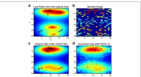
In this scenario, the rate of sensing per node is insuffi-cient and the field changes within one collection interval sinceT >Tcoh. Thus, the per-node sensing rateλ1sneeds to be increased. The targets are no longer steady within the duration of a collection intervalTleading to blurring, which makes target detection challenging. The estimation task in this case is further complicated by the fact that the packets from different frames may have been collected during the interval T. This scenario leads to a violation of the stationarity assumptions made initially. The recon-structed map is thus blurred because of different packets

originating from different frames (Fig. 3). In this case, we use a specific error metric based on model fitting to estimate the reliability of reconstruction and object detection.

4 Simulation of a sample dynamic field

In this paper, we demonstrate the adaptive monitor-ing procedure usmonitor-ing a sample model for the field. We demonstrate our adaptive scheme to adjust the per node sensing rate in RACS using a simulated example field in this paper. Using a realistic example allows us to control the coherence parameterTcohand monitor the effect of

changing the collection intervalTin accordance with the adaptive algorithm.

We first describe the example field that serves as our test case. Suppose, a field with M targets is being observed. Each target in the field is assumed to generate a signature (e.g., heat, sound, etc) decaying exponentially with distance from its location. At time t, the process observed by sensor nodeiat coordinate(xi,yi)is given by Eq. (3)

ui(t)= M

m=1 Ame−p

√

(xi−am(t))2+(yi−bm(t))2 ₍₃₎

where am(t) and bm(t) are the coordinates of the mth target at time t, Am is its strength, and p is the decay rate of the sources. The process then evolves over time as the sources move along random tra-jectories. Similar models are commonly found in the energy-based localization literature for static sensor net-works [20–22] when the targets being detected are not moving.

x

y

1

2 3

4

Last frame from the original map

5 10 15 20 10

20

30

40

50

Sensed image

5 10 15 20 10

20

30

40

50

original map under motion blur

1

2 3

4

5 10 15 20 10

20

30

40

50

recovered map after frame 10

5 10 15 20 10

20

30

40

50

d

c

b

a

Fig. 3 a–dThe effect of the field changing at rate faster than the sensing rate.ais the original undistorted map that was sensed atTcohwhile (c) shows the same field obtained through temporal blurring after an observation intervalT=10×Tcoh.dis the field obtained as a result of sensing at a rate 10 times slower than the field’s underlying rate of change. Notice how (d) is more similar to the blurred map (c) than (a). This distortion in the sensed field is an example of undersensing

λinit

1s . The initial sensing rate is determined using histor-ical data by setting the desired parameters in Eq. (2). Once the map of the fieldGsa_{is recovered using sparse} approximation techniques, the FC may now use the rate adjustment algorithm described later to decide if the sensing duration T needs to be adjusted. The sen-sors employ the adjusted sensing rate in the ensuing sensing duration. In this paper, we discuss metrics for the proposed rate adjustment algorithm for this family of field models, although the framework itself is quite general.

For simulating a map of the field as defined above, we start with a set of randomly chosen parameters. In addi-tion, each target is assigned a random velocity and direc-tion of movement. To simulate theundersensingcase, we consider that collection occurs over Nb coherence time intervals (referred to as frames) whereT ≈ N_bTcoh. The

randomly sampled packets are then collected uniformly over the lastNbframes (Fig. 3). This effectively leads to motion blurring of the targets as mentioned before. To simulate the oversensing case, the collection interval is reduced toT=Tcohwhile each target’s velocity is scaled

byT/Tcohto make them appear to be moving slower. To

deal with the issue of a finite field size, targets moving out of the field are replaced by new targets starting from the same location assigned a new random velocity and direction.

5 Adaptive field monitoring scheme

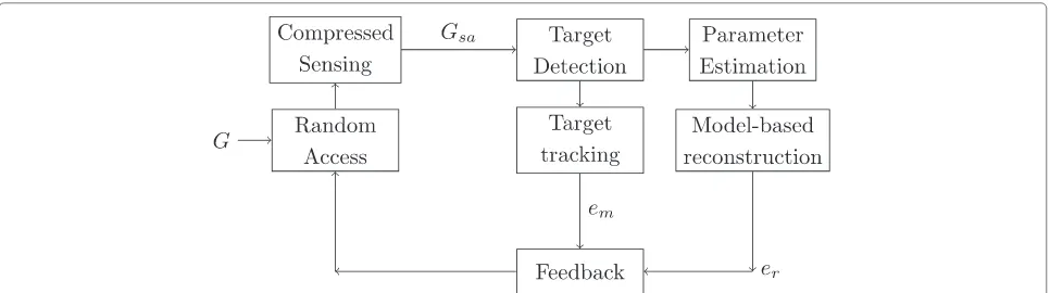
In this section, we discuss specific algorithms and met-rics extracted using the reconstructed map, which are used for the adaptive rate control of per-node sensing in RACS. Although the algorithms discussed below have been adapted to this particular family of models used in the simulation example, we have attempted to lay-out broad steps whenever possible and provide a general scheme to be used in such cases. These algorithm stages have been presented in the block diagram shown in Fig. 4.

5.1 Target localization

Before taking any decisions about the current sensing state, we first detect and localize the targets in the image. Similar to [18], by involving target detection in the feed-back process, we would like to ensure that the rate of sensing is optimized for the end goal of target detection.

Fig. 4Block diagram for the adaptive feedback mechanism.Gdenotes the true measurements on the time varying field

in this process using a sparsity constraint. However, the method still depends on exact knowledge of the field model.

To overcome this drawback, we propose a target local-ization algorithm based on local gradient ascent. The proposed method only requires that the target signatures be monotonically decaying away from the target. This technique is adapted from the mode seeking mean shift algorithm [23] which is frequently used for unsupervised clustering of data. Consequently, it can be interpreted as searching local peaks in the data histogram. In the task at hand, we are instead interested in finding local peaks in field intensity. We also modify the algorithm slightly to adapt to the discrete search space for this problem. Specif-ically, we start from a random initial pointXon the map. A mean-shift-based gradient ascent technique is then used to update the location of this point in each iteration till a peak is found. Given the current locationX, we estimate an intensity weighted meanXcfor locations aroundXin a window of sizeWas shown in Eq. (4). Note that the direc-tion fromX toXc gives the direction of gradient ascent, along whichXshould be updated in the next iteration.

However, in the current problem, we are working on a space of discrete sensor locations. To make the algo-rithm better suited to such a scenario, we quantize the gradient direction to eight angular bins. Depending on the direction of the gradient, X is then shifted to one of its eight connected points. This process is explained using a schematic in Fig. 5. The iterations are repeated until

Xconverges to a local maximum or reaches a point that has already been visited. The entire procedure is repeated multiple times with new random initial points till the peaks have been discovered. In practice, it is not necessary to traverse all points in the field to discover all the peaks (Fig. 6), and we restrict the algorithm to a fixed number of iterations. The parameterW in this algorithm serves as a mask over which the gradient can be estimated more robustly. The target detection procedure is explained in Algorithm 1.

Algorithm 1: Modified gradient ascent algorithm for target detection on the acquired map. (See Fig. 6)

Input:P×QmapGsa_{reconstructed by RACS} Output: Location of targetsμ1,μ2,. . .where the

number of targets is initially unknown Set maximum number of iterations toM, size of window toW

Cluster indexK←1 foriter ←1toMdo

Randomly select an initial locationXon the map. whileXhasn’t already been visiteddo

MarkXas visited and belonging to clusterK //assuming we’re going to find a new target

Compute the new center of massXcwithin a window of sizeWaroundX.

Compute the direction fromXtoXcand quantize it into 8 bins between

{−π/8,π/8, 3π/8. . .}(Fig. 5)

Update the position ofXto one of the 8 adjacent positions based on the quantized direction (Fig. 5)

end while

Mark all points in this trail leading uptoXas belonging to the same cluster asX

ifXbelongs to the new clusterKthen AppendXasμK to the set of targets

//new target found

K←K+1

end if end

Xc= s

I(s)K(s−X)s

s

I(s)K(s−X),s∈P×Qgrid

K(s−x)=

1 if||s−x||c≤W

Fig. 5Modified discrete step update scheme using quantized directions.Asterisk(*) indicates points on the grid.Idenotes theP×Q

grid of intensity values, andK(.)denotes our particular choice of kernel function used for computing mean

5.2 Parameter estimation

Once the positions am and bm for the targets have been identified using the target localization algorithm described above, we try to obtain a minimum mean square error (MMSE) estimate of the field parameters defined in Eq. (3) using a method of comparison by synthesis to match the acquired mapGsa_{against a model. The} param-eters of model denoted by Gmodel _{comprise the target}

locations(am,bm), their respective strengthsAm, and the decay parameters of the target signature (p).

We estimate the parameters using a nonlinear regres-sion [24] technique to optimize an MMSE formulation as

shown in Eq. (5). We use thenlinfitfunction in MATLAB for solving this optimization problem. Since the optimiza-tion is not convex, the choice of initial points is important. We use the target localizations estimated earlier and a reasonable value for the decay as our initial point. The estimated parameters are then used to generate a map of the fieldGdet(Fig. 7d). Gdet represents what the control algorithm expects the field to look like based on the target localizations and its knowledge of the model.

a,b,A,p= arg min

am,bm,Am,p

P

i=1

Q

j=1

_M

m=1

Gmodelij (am,bm,Am,p)−Gsaij

2

(5)

Gdet=Gmodel(a,b,A,p) (6)

5.3 Reliability metric for reconstruction

We obtain a reliability metric for reconstruction based on the error in the model fitting described above. We com-pare the model-based mapGdetagainst the non-model-based map Gsa recovered via sparse approximation by projecting both of them on the DFT matrix and decom-posing the error into a high-frequency (HF) and low-frequency (LF) term. The intuition is thatGsashould be similar toGdet, but for any errors resulting from issues in either sensing or localization. A gross mismatch between the coefficients will be captured by the LF term indicat-ing an inaccurate detection while a large value of the HF term (denoted byer) is a characteristic of a poor recon-struction due to violation of the assumptions in RACS (Fig. 8a, b). The definition of this error term is shown in Eq. (7) whereF_Hdenotes a 2D high-pass filter, ander is obtained by convolving it with the difference between the imagesGdetandGsa. The cutoff frequency for the filters can be chosen from a previous estimate of the field. The error metricer thus comes in handy in theundersensing

x

y

1 2

3 4

Original map with different components

5 10 15 20

10

20

30

40

50

Sensed image

1 2

3 4

5 10 15 20

10

20

30

40

50

map reconstructed via RACS

5 10 15 20

10

20

30

40

50

map recovered after detection

5 10 15 20

10

20

30

40

50

a

b

c

d

Fig. 7Steps in rate adjustment.bshows the samples chosen at random, and (d) is the map generated using the parameters estimated on (c). Notice how (d) is approximately similar to (a) when detection is accurate

case when the acquired mapGsais either blurred or poorly reconstructed.

er=FH∗

Gdet−Gsa

(7)

5.4 Measuring motion by target tracking

In addition to compensating for the dynamic nature of the field in theundersensing case, we would also like to eliminate any redundant sensing. Recall, that in the over-sensingcase, the field changes very slowly, yielding perfect reconstruction and detection. This makes it necessary to monitor the field over multiple frames for detecting any signs ofoversensing.

To quantify motion in the field, we track the loca-tion of detected targets over the last L frames. Note that this is not trivial since the number of targets detected is not guaranteed to be consistent from one frame to another. Moreover, the target indices assigned by the detection algorithm are non-unique. To deal with this issue, we use a tracking approach based on dynamic programming that ensures tracking even if the object is not detected in some of the intermedi-ate frames. More specifically, we recursively minimize the total distance moved by a target over L frames. If the targets are spaced sufficiently apart, this ensures

tracking of the slowest moving target over multiple frames.

Suppose

ˆ

at_i,bˆt_i

denote the location of the ith target detected in frametand letdt_ijbe defined as the distance between the ith target detected in the frame t and the

jth target detected in the framet+1. Then the net dis-tanceD(n1,n2,. . .,nL)moved by a target overL frames and detected at the indices {n1,n2,. . .,nL} is given by Eq. (8).

D(n1,n2,. . .,nL)= L−1

t=1

dt_ntnt+1; 1≤nt≤Mt (8)

dt_ij=

at_i−at_j+1

2

+bt_i−bt_j+1

2

(9)

0 500 1000

T coh

(in s)

0 200 400 600

Tcoh

(in s)

20 40 60 80 100 120 140 160 180 200 0 50 100

Error HF

Time

0 20 40 60 80 100 120 140 160 180 200 0 50 100 150

Error LF

Time

LF e det T

coh T

T coh T HF e

det

a

b

0 500 1000

Tcoh

(in s)

20 40 60 80 100 120 140 160 180 200 0 5 10

tracking−based−metric

Time

T coh T

tracking−based L=10

0 200 400 600

T coh

(in s)

0 20 40 60 80 100 120 140 160 180 200 0 5 10 15

tracking−based−metric

Time

T coh T

tracking−based L=5

c

d

Fig. 8 aHF andbLF components of the model-based error and the minimum average motion per frame for (c)L=5 and (d)L=10 cases. The system is in open-loop control, i.e., the error metrics are not being compensated for which can be noted by the flatTline

to be much higher when the objects get blurred in the

undersensingcase.

em= 1

Lnmin1,...,nL

D(n1,. . .,nL) (10)

6 Feedback algorithm for rate adjustment

After computing the error metricser andem, a control algorithm is used to determine if the current sensing rate needs to be changed. This information is fed back to the FC which makes any necessary changes to the sens-ing rate, thereby establishsens-ing a closed-loop control. The objective of control is to minimize the reconstruction error-based metricer at the same time ensuring that the targets move significantly from frame to frame as indi-cated by the tracking error metricer. This ensures that the system is in a sweet spot betweenundersensing and

oversensing.

In this paper, we propose a dual threshold feedback scheme to keep the system in this “optimal” state. We define two parameters: a lower thresholdthmfor the met-ricem and an upper thresholdthr forer, respectively. In the proposed scheme, the value of these two parameters is tuned adaptively. The control algorithm itself consists of two modes: an “adjust” mode and a “calibrate” mode. The system’s current mode is decided based on which of the four system states (A–D) it currently is in. These system states are shown in Fig. 9.

In the adjust mode (states A and D in Table 1), the collection interval T is incremented or decremented by a scalar update (κ > 1) depending on the value of the metrics. In state A, the conditionem≤thmindicates

over-sensingand hence the algorithm would decide to increase

Fig. 9Four states of the control algorithm as determined by the error metricserandembased on the thresholdsthrandthm. The ideal

operating zone is shown by theshaded region

thereby increasing the sensing rate. The mutually oppos-ing nature of these two conditions gives rise to a “stable” or buffer region forT(see Table 1) where it is not updated. In this mode, we only adapt the width of the buffer region by adjusting the threshold values such that for the current value ofT, the control is just within the stable zone. Note, that it might not be feasible to guess a value forthmorthr making this adaptive approach necessary.

In practice, the thresholds can be initialized to extreme values such that the buffer region is wide enough and the system is guaranteed to start in state B. In subsequent intervals, the thresholds are updated in the “calibration” mode to shrink this buffer region. The ideal operating zone, centered at(thr,thm), is shown by a shaded region in Fig. 9. If the system steps out of this operating zone, the thresholds are adjusted in a direction such that the cur-rent system state is contained within the operating zone. In the calibration mode, the thresholds are adjusted by

predefined stepsαandβsuch that the system stays within the operating zone. In other words, the aim of this adap-tive control is to obtain the tightest stable region of control forT.

To provide an intuition of how the scheme works, con-sider the graphical illustration of the proposed feedback algorithm in Fig. 9. At any time instant, the system state can be represented as a point on theeremplane. The rel-ative position of this point with respect to the thresholds

thr and thm is then used to decide the next course of action. In general, the algorithm tries to maintain a narrow buffer region of control by keeping the operating point (er,em)close to(thr,thm). This can be achieved by either updating the sensing time periodT (states A and D) or by adapting the thresholds (states B and C).

By observing how the states of the algorithm transition, we present an argument to show that the proposed algo-rithm is bounded-input bounded-output (BIBO) stable. This means that for a finite coherence timeTcoh, the

con-trolled variable viz. the sensing time periodT is always bounded. This can be shown by considering each of the four states of operation A, B, C, and D of the proposed algorithm above.

Suppose, we are currently in state A (oversensing) and the feedback algorithm responds by increasing T. This leads to an increase in bothem ander since fewer sam-ples are sensed per unit time. This, in turn, prevents the system from staying in state A and is most likely to cause a transition to states B or C. Similarly, if the sys-tem is in state D (undersensing), the algorithm responds by decreasingT. This leads to the net effect that bother andem decrease, taking the system out of state D. When the system is in states B or C, the thresholds are var-ied so that operating point is maintained close to the adapted thresholds. This ensures that the sensing time periodT and in turn the error metricser andem cannot grow unbounded for a given finite Tcoh. As an

exam-ple, note the state transitions in Fig. 10 which shows the internal states of the algorithm for a simulated control scenario.

Table 1Control feedback rules (“adjust” mode: A, D ; “calibrate” mode: B, C)

Oversensing

em<thm

Stable region Undersensing

er>thr

State A B C D

Condition em<thm em>thm em<thm er>thr

er<thr er<thr er>thr em>thm

Decision T↑ Narrow Widen T↓

Update T=κT thr = thr − α

thm=thm+β

thr = thr + α

thm=thm−β

0 500 1000

T coh

(in s)

20 40 60 80 100 120 140 160 180 200

A B C D

State

Time Tcoh

T System State

Fig. 10Figure shows the internal states of the algorithm as it makes various rate adjustment decisions. States are the same as described in Table 1

7 System operation

We presented an example of the control system in an open-loop operation earlier in Fig. 8 which showed the value of metrics er andem for a particular Tcoh profile.

Figure 8c, d suggests that a largerLmight be related to a slower response time ofemas can be seen aroundt=80, 100 when the field’sTcohchanges. The error metrics based

on model fitting (Fig. 8a, b) are computed from the current frame and thus respond instantaneously to the changes in field coherence. It is also worth noting here that the HF errors (spatial high-frequency component) typically correspond to the reconstruction error in the undersens-ing case, while the LF error serves as a sanity check for detection.

In this section, we present an example of closed-loop control by using the feedback mechanism (Table 1) dis-cussed earlier to compensate for the error metrics as shown in Fig. 11. Note that the collection time interval

T now attempts to trace the underlying hidden parame-terTcohas the system tries to keep botherandemwithin bounds. Figure 10 provides a better insight into the system by showing the feedback algorithm’s underlying internal state. Recall that states A and D correspond to oversensing

and undersensing respectively while in states B and C, the thresholds are adapted to achieve a tight buffer region of stability.

8 Simulation results

We run simulations with M = 4 targets and different velocity and decay parameters, using the proposed feedback algorithm for sensing rate adjustment. We evaluate the performance of the algorithm using two different criteria. First, the average mean squared error (MSE) between the estimated sampling durationT (blue line in Fig. 11) and the coherence time ground truth

Tcoh (red line in Fig. 11) is computed as a measure of

the algorithm’s ability to track and adapt to changes in coherence time. Secondly, we calculate the F-score measure for target detection in each frame. This is a reasonable criterion for our task since the end goal of such an application would be target detection and tracking. To calculate the F-score of target detection in a frame, we check how many of the localized targets correspond to actual target locations. F-score weights both the precision and recall of target detection as follows

0 500 1000

Tcoh

(in s)

0 200 400 600 800 1000

Tcoh

(in s)

0 50 100 150 200 2500

20 40

er

Time

T_coh T model−error

0 50 100 150 200 2500

2 4 6 8 10

em

Time

T_coh T

tracking−based L=5

Precision= # targets that were correctly localized # targets that were localized

Recall= # targets that were correctly localized # targets actually present

F= 2.Precision.Recall

Precision+Recall (11)

8.1 Baseline algorithm

We compare the results against a baseline method based on correlation of the currently acquired fieldGsawith the field acquired in the previous cycle as suggested in [15]. Control decisions are taken depending on twofixedhigh (δh) and low (δl) thresholds on the correlation value. T is incremented if correlation exceedsδhand decremented if correlation falls below δl. T is not updated if corre-lation lies between these two thresholds. The sampling duration T is changed using a scaling parameter κ as earlier.

Figure 12 shows the results of our simulation for the baseline and proposed methods. The results, averaged for each run, are shown for different parameter settings of velocity and decaypas defined in Eq. (3). Remember that a high F-score indicates accurate target detection while a low MSE denotes accurate tracking of the underlying coherence time (Tcoh).

Figure 12a shows the results for the baseline method using correlation as a feedback metric. From the MSE andF-score plots, it is evident that the baseline algorithm performance drops with increase in decay parameter p. This is expected since the targets with a lesser spread do not affect the correlation metric significantly. In contrast,

for our proposed feedback algorithm, the performance improves with increase in the decay parameterpsince tar-gets with lesser spread are easier to localize and hence field reconstruction is more accurate (Fig. 12b). A simi-lar trend can be seen for average MSE which is related inversely to the target detectionF-score. In other words, this might indicate that poor tracking of the underlying

Tcoh is related to poor target detection, thereby making

a case for the proposed sensing rate adjustment in this paper.

Since velocity for each target is assigned uniformly at random in the simulation, we control the velocity range that can be assigned to each target as a parameter instead. We note that increase in velocity has a positive influence on the performance of both the algorithms. This can be easily explained by considering that an increase in velocity of the targets makes it easier to discriminate between the oversensing, adequate sensing, and undersensing states. This holds for both the algorithms, and hence, we notice a general increase inF-score and decrease in MSE with increase in velocity. Finally, we also note that our pro-posed detection-based feedback mechanism outperforms the baseline correlation-based method in terms of the accuracy of target detection as indicated by the higher

F-score. The average target detection F-score obtained for the baseline algorithm was 0.32 while our proposed method achieved an averageF-score of 0.45.

8.2 Simulations with measurement noise

Next, we test the noise robustness of our proposed method by adding synthetic sensor or measurement noise

decay

to the field. We simulate measurement noise by adding zero mean white Gaussian noise at different amplitudes (σnoise) while keeping the original field’s intensity the

same. Results are averaged on full runs for different noise level, and the F-score for target detection accu-racy is shown in Fig. 13. Other simulation factors such as velocity-scale and decay were held constant at 1 and 0.3 respectively for the purposes of this simulation.

The results show a clear degradation inF-score for both the proposed detection-based and baseline correlation-based methods, as the SNR decreases. However, we note that for the baseline algorithm, theF-score initially increases with decrease in SNR hinting at suboptimal-ity in processing. On further investigation, we found this peculiar trait to be an artifact of the control algorithm and the choice of metric used in the baseline scheme. As noise is added to the field value of the correlation metric drops, which leads the FC to confuse the current state as undersensing. This inference leads to a monotonic decrease in sampling durationT, temporarily increasing performance at the cost of energy efficiency. The target detection F-score peaks around σnoise = 0.05 beyond

which the accuracy of target-detection algorithm is signif-icantly affected. On the other hand, this artifact does not affect the proposed method significantly, since the met-ric used for our control algorithm is based directly on target detection. As a result, we note that our proposed method exhibits a more graceful degradation in perfor-mance with increase in noise without compromising on energy efficiency.

9 Conclusions

In this work, we present a rate adjustment scheme for random access compress sensing (RACS) to monitor and

compensate for the rate of change in time-varying fields. Adjustment of sensing rate for RACS is motivated by the trade-off between energy efficiency and the accuracy of tracking targets of interest. Although direct estimation of the coherence time might seem to be the best approach for sensing a time varying field, we note that it is not directly related to our end goal of target detection in the field. We also observe that the reconstruction error in RACS has a complex relation to the current coherence time of the field and factors like the position of targets, their velocity, etc. Thus, by making the algorithm depend on the detec-tion and localizadetec-tion of targets, we ensure that the rate adjustment is tied in to our actual objective.

In this paper, we propose two unsupervised metrics to inform the rate adjustment scheme. A model-based field reconstruction is done after target localization for each acquired frame, and the model fit errorer is used as a metric to detect cases when the FC is undersensing. To account for oversensing in operation, we define a measure for the motion of detected targets in the pastL frames. This motion based metricemindicates any redundancy in sensing and can be used to decrease the collection time intervalTif needed.

We proposed a dual-threshold-based feedback mech-anism using these error metrics for rate sensing adjust-ments. The technique assumes minimum prior knowledge and adapts the threshold in an online fashion using rea-sonable assumptions about the field. We also show that the proposed control mechanism is BIBO stable. In addi-tion, we compare our results against a baseline algorithm that uses temporal correlation of the acquired fields and show that the proposed rate adjustment mechanism per-forms better on an average in terms of target detection accuracy even in the presence of noise.

0 0.02 0.04 0.06 0.08 0.1 0.12 0.14 0.16 0.37

0.375 0.38 0.385 0.39 0.395 0.4 0.405 0.41 0.415 0.42

σ_noise

F−score

Detection−based correlation−based

Endnote

1_{We use the termstationaryin this paper to refer to}

fields that are temporally static during the sensing duration.

Competing interests

The authors declare that they have no competing interests.

Acknowledgements

This work was supported by ONR and NSF.

Author details

1_{Signal Analysis and Interpretation Laboratory (SAIL), Electrical Engineering,}

University of Southern California, Los Angeles, CA, USA.2Department of Electrical and Computer Engineering, Northeastern University, Boston, MA, USA.

Received: 20 July 2015 Accepted: 7 April 2016

References

1. EJ Candes, J Romberg, T Tao, Stable signal recovery from incomplete and inaccurate measurements. Comm. Pure Appl. Math.59, 1207–1223 (2005) 2. EJ Candes, J Romberg, T Tao, Robust uncertainty principles: exact signal

reconstruction from highly incomplete frequency information. IEEE Trans. Inform. Theory.52, 489–509 (2006)

3. E Candes, J Romberg, Sparsity and incoherence in compressive sampling. Inverse Problems.23, 969–985 (2006)

4. WU Bajwa, J Haupt, AM Sayeed, R Nowak, in5th Int. Conf. Information Processing in Sensor Networks (IPSN’06). Compressive wireless sensing, (2006), pp. 134–142

5. WU Bajwa, J Haupt, AM Sayeed, R Nowak, Joint source-channel communication for distributed estimation in sensor networks. IEEE Trans. Inform. Theory.53(10), 3629–3653 (2007)

6. CT Chou, R Rana, W Hu, inIEEE 34th Conference on Local Computer Networks (LCN). Energy efficient information collection in wireless sensor networks using adaptive compressive sensing, (2009), pp. 443–450 7. C Luo, F Wu, J Sun, CW Chen, inProceedings of the 15th Annual

International Conference on Mobile Computing and Networking.MobiCom. Compressive data gathering for large-scale wireless sensor networks, (2009), pp. 145–156

8. J Meng, H Li, Z Han, in43rd Annual Conference on Information Sciences and Systems (CISS). Sparse event detection in wireless sensor networks using compressive sensing, (2009), pp. 181–185

9. R Masiero, G Quer, D Munaretto, M Rossi, J Widmer, M Zorzi, in Proceedings of the 28th IEEE Conference on Global Telecommunications. GLOBECOM’09. Data acquisition through joint compressive sensing and principal component analysis, (2009), pp. 1271–1276

10. R Masiero, G Quer, M Rossi, M Zorzi, inICUMT’09. A Bayesian analysis of compressive sensing data recovery in wireless sensor networks, (2009), pp. 1–6

11. S Lee, S Pattem, M Sathiamoorthy, B Krishnamachari, A Ortega, in GeoSensor Networks.Lecture Notes in Computer Science.

Spatially-localized compressed sensing and routing in multi-hop sensor networks, vol. 5659 (Springer, 2009), pp. 11–20

12. D Motamedvaziri, V Saligrama, D Castanon, inCommunication, Control, and Computing (Allerton), 2010 48th Annual Allerton Conference On. Decentralized compressive sensing, (2010), pp. 607–614

13. F Fazel, M Fazel, M Stojanovic, Random access compressed sensing for energy-efficient underwater sensor networks. IEEE J. Selected Areas Commun. (JSAC).29(8), 1660–1670 (2011)

14. F Fazel, M Fazel, M Stojanovic, Random access compressed sensing over fading and noisy communication channels. Wireless Commun. IEEE Trans. 12(5), 2114–2125 (2013)

15. F Fazel, M Fazel, M Stojanovic, inInformation Theory and Applications Workshop (ITA), 2012. Random access sensor networks: field reconstruction from incomplete data (IEEE, 2012), pp. 300–305 16. S Reed, Y Petillot, J Bell, An automatic approach to the detection and

extraction of mine features in sidescan sonar. Oceanic Eng. IEEE J.28(1), 90–105 (2003)

17. N Kumar, QF Tan, SS Narayanan, inAcoustics, Speech and Signal Processing (ICASSP), 2012 IEEE International Conference On. Object classification in sidescan sonar images with sparse representation techniques (IEEE, 2012), pp. 1333–1336

18. K Kerse, F Fazel, M Stojanovic, inSignals, Systems and Computers, 2013 Asilomar Conference On. Target localization and tracking in a random access sensor network (IEEE, 2013), pp. 103–107

19. JA Tropp, SJ Wright, Computational methods for sparse solution of linear inverse problems. Proc. IEEE, Special Issue, Appl. Sparse Representation and Compressive Sensing.98(6), 948–958 (2010)

20. D Li, YH Hu, Energy-based collaborative source localization using acoustic microsensor array. EURASIP J. Appl. Signal Process.2003, 321–337 (2003) 21. X Sheng, Y-H Hu, Maximum likelihood multiple-source localization using

acoustic energy measurements with wireless sensor networks. Signal Process. IEEE Trans.53(1), 44–53 (2005)

22. W Meng, W Xiao, L Xie, An efficient em algorithm for energy-based multisource localization in wireless sensor networks. Instrum. Meas. IEEE Trans.60(3), 1017–1027 (2011)

23. Y Cheng, Mean shift, mode seeking, and clustering. Pattern Anal. Mach. Intell. IEEE Trans.17(8), 790–799 (1995)

24. PW Holland, RE Welsch, Robust regression using iteratively reweighted least-squares. Commun. Statistics-Theory Methods.6(9), 813–827 (1977)

Submit your manuscript to a

journal and benefi t from:

7Convenient online submission

7Rigorous peer review

7Immediate publication on acceptance

7Open access: articles freely available online

7High visibility within the fi eld

7Retaining the copyright to your article