EXPRESS LETTER
Gravity gradient tensor analysis to an active
fault: a case study at the Togi-gawa Nangan
fault, Noto Peninsula, central Japan
Yoshihiro Hiramatsu
1*, Akihiro Sawada
1, Wataru Kobayashi
2, Satoshi Ishida
2and Masaaki Hamada
2Abstract
Gravity gradient tensor analysis has been a powerful tool for investigating subsurface structures and recently its application to a two-dimensional fault structure has been developed. To elucidate the faulting type and spatial extent, specifically the continuity and the size, of the subsurface fault structure of an active fault through gravity gradient tensor analysis, we analyzed Bouguer anomalies, which were composed of dense gravity measurement data over the land and seafloor, and indices calculated from a gravity gradient tensor around the Togi-gawa Nangan fault (TNF), Noto Peninsula, central Japan. The features of Bouguer anomalies and their first horizontal and vertical derivatives demonstrate clearly that the TNF is a reverse fault dipping to the southeast. Furthermore, the combination of those derivatives and the dimensionality index revealed that the spatial extent of the subsurface fault structure is coinci-dent with that of the surface fault trace and that it shows no evidence of connecting the TNF with surrounding active faults. Furthermore, the dip angle of the subsurface fault structure was estimated as 45°–60° from the minimum eigenvectors of the gravity gradient tensor. We confirmed that this result is coincident with the dip angle estimated using the two-dimensional Talwani’s method. This high dip angle as a reverse fault suggests that the TNF has experi-enced inversion tectonics.
Keywords: Active fault, Bouguer anomaly, Dip angle, Two-dimensional Talwani’s method, Inversion tectonics
© The Author(s) 2019. This article is distributed under the terms of the Creative Commons Attribution 4.0 International License (http://creat iveco mmons .org/licen ses/by/4.0/), which permits unrestricted use, distribution, and reproduction in any medium, provided you give appropriate credit to the original author(s) and the source, provide a link to the Creative Commons license, and indicate if changes were made.
Introduction
Elucidating the subsurface fault structure of an active fault is important for understanding regional tecton-ics and seismic risks. Geophysical surveys are useful for investigating subsurface structures. Fault movements dis-place the basement, causing gravity anomalies around an active fault. Especially, vertical displacement of the base-ment causes a steep change in Bouguer anomalies across the fault. Therefore, the first horizontal derivative (HD) and the first vertical derivative (VD) of Bouguer anoma-lies are often used to highlight subsurface fault struc-tures. Wada et al. (2017), based on the continuity of high HD and the zero isoline of VD for two active fault zones on the east margin of the Niigata Plain in central Japan,
inferred that subsurface fault structures are continuous. Recently, other methods to investigate the subsurface fault structure, especially for the dip angle of a fault, have been developed using the gravity gradient tensor (Kusu-moto 2015, 2017). For the 2016 Kumamoto earthquake in Japan, Kusumoto (2016) used eigenvectors of the gravity gradient tensor to estimate the dip angle of the Kuma-moto-Ooita tectonic line, which includes the source fault of the earthquake, as approximately 65° (Beiki and Ped-ersen 2010). Matsumoto et al. (2016) also analyzed grav-ity data around the 2016 Kumamoto earthquake source fault and discussed the faulting type and segmentation of the source fault through features obtained from the grav-ity gradient tensor. Nevertheless, reported applications of the gravity gradient tensor to analyses of the subsurface structure of active faults are few. More case studies must be conducted to examine its effectiveness.
The study area is the western Noto Peninsula, central Japan, where dense gravity surveys have been conducted
Open Access
*Correspondence: [email protected]
1 School of Geosciences and Civil Engineering, College of Science
and Engineering, Kanazawa University, Kakuma, Kanazawa, Ishikawa 920-1192, Japan
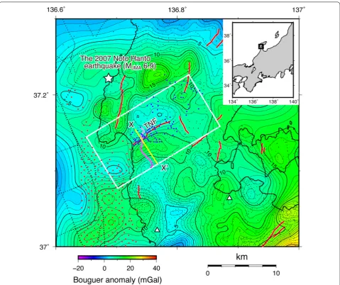
mainly by Kanazawa University (Honda et al. 2012) (Fig. 1). The Noto Peninsula is composed mainly of Oli-gocene to Early Miocene volcanic rocks and post Oligo-cene sediment rocks (e.g., Kaseno 1993) (Fig. 2). These volcanic rocks erupted during the rifting event of the back-arc basin of the Japanese islands. The rifting ceased during the Middle Miocene. This rifting formed normal faults around the Noto Peninsula. Some of the normal faults have been reactivated as reverse faults because of the compressive stress associated with forearc subduc-tion (e.g., Katagawa et al. 2005).
Active Fault Research Group (1991) reported several active faults in this area, such as the Togi-gawa Nangan fault (TNF) (Figs. 1 and 2). Based on geomorphological features, Active Fault Research Group (1991) reported that the TNF is a reverse fault with uplift on the south-eastern side. Imaizumi et al. (2018) extended the eastern end of the TNF through re-evaluation of geomorphologi-cal features (Figs. 1 and 2). This fault is located along the boundary between late Pleistocene to Holocene sedi-ments/sand dune deposits and Miocene andesite on the ground surface (Fig. 2).
This study conducted a dense gravity survey and cre-ated a detailed gravity anomaly map around the TNF. We elucidate features of gravity anomalies and indices derived from the gravity gradient tensor around the TNF and discuss the faulting type, the continuity and size, and the dip angle of the TNF.
Data and method
Gravity measurement, compilation, and corrections
Gravity data used for this study consist mainly of two datasets. The first comprises data measured on land; the second includes data of the seafloor (Fig. 1). We con-ducted a gravity survey on land, around TNF using a Scintrex CG-3M gravimeter from February 26 through
September 11 in 2018 and obtained 279 gravity data (Fig. 1). For analysis of the two-dimensional density structure, we set a profile across the TNF and conducted a gravity survey with an interval of 25–50 m and to a maximum 173 m on the profile (Fig. 1). The positions of gravity measurement points were obtained from Global Navigation Satellite System (GNSS) observations. In the case of poor location of GNSS, that is, the solution is not fix, we used a 10-m mesh digital elevation model (DEM), published by the Geospatial Information Author-ity of Japan, for locating. For the points on the profile, we used a total station for locating. Gravity measurement of the seafloor was conducted by Hokuriku Electric Power Company from May 20 through June 20 in 2018 (Ishida
et al. 2018). They used a Scintrex INO ocean bottom gravity meter to obtain 275 gravity data in an approxi-mately 40 km × 10 km area west of the Noto Peninsula (Additional file 1: Figure S1). The points presented in Fig. 1 do not cover all areas for which gravity measure-ments were conducted on the seafloor. These gravity data from the seafloor filled a clearly apparent gap left by ear-lier gravity measurement data published by the Geologi-cal Survey of Japan (2013) and Murata et al. (2018) for the sea area (Fig. 1).
In addition to the data described above, we com-piled gravity data reported by the Geographical Survey Institute (2006), Yamamoto et al. (2011), Honda et al. (2012), and the Geological Survey of Japan (2013). Data of the Geological Survey of Japan (2013) include data of shipboard gravity measurements described above. We applied terrain correction with the 10-m mesh DEM, and a plain trend correction, together with normal correction procedures (e.g., tide, drift, free-air, and Bouguer cor-rections), to the compiled gravity data. The values of the density used for the terrain and the Bouguer corrections are 2300 kg/m3 because we used Bouguer anomaly data
created from the shipboard gravity measurements with correction density of 2300 kg/m3 (Geological Survey of
Japan 2013). These values are close to the optimum cor-rection density of 2350 kg/m3 in the large area including
most of the Noto Peninsula (Murata et al. 2018). Further-more, we applied a low-pass filter with a cut-off wave-length of 3000 m to the Bouguer anomalies as a Bouguer anomaly map for the analysis of the gravity gradient ten-sor (Fig. 1).
Estimation of gravity gradient tensor and related indices
The gravity gradient tensor is defined by the partial deriv-atives of the gravity vector (gx, gy, gz) as
Assuming a Bouguer anomaly as gz, as measured on the x–y plane, the gravity gradient tensor is calculated using the Fourier transform of gz as proposed by Mickus and
Hinojosa (2001). From the gravity gradient tensor, the first horizontal derivative (HD), the first vertical deriva-tive (VD), and the normalized total horizontal derivaderiva-tive (TDX) (Cooper and Cowan 2006) are defined as
(1)
These indices are useful to detect a subsurface density discontinuity such as a fault structure. The strike and dip angles of a two-dimensional causative body can be esti-mated from the minimum and maximum eigenvectors of a gravity gradient tensor (Beiki 2013). Kusumoto (2015) demonstrated that the dip angle of a fault plane can be estimated from the maximum eigenvector. Recently, Kusumoto (2017) demonstrated from a numerical simu-lation that the dip of the minimum eigenvector followed the dip of a reverse fault. Using the minimum eigenvec-tor, he estimated the dip angle of a reverse fault in central Japan: the Kurehayama fault. He emphasized the impor-tance of the selection of the eigenvector by consideration of the faulting type: a normal fault or a reverse fault. For a reverse fault, the dip angle defined by the minimum eigenvector of a gravity gradient tensor ( ν3x,ν3y,ν3z ) is
given as
The geological setting of this study area is similar to that of Kusumoto (2017). We therefore used this formu-lation to estimate the TNF dip angle. The dimensionality index Di is defined by using the eigenvalues 1,2,3 , of a
gravity gradient tensor as
where I1=12+23+13 and I2=123
(Ped-ersen and Rasmussen 1990). Di indicates whether the
subsurface structure is approximately two-dimensional (Di approaches 0) or three-dimensional (Di approaches
1).
Two‑dimensional Talwani’s method
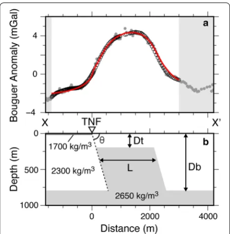
In addition to the gravity gradient tensor analysis, we applied the two-dimensional (2D) Talwani’s method (Tal-wani et al. 1959) to verify the subsurface density struc-ture of the TNF, especially for the dip angle, obtained through gravity gradient tensor analysis. The Bouguer anomaly data for the 2D density structure analysis were produced from the gravity data measured on the profile traversing the TNF (Fig. 1). We set a line across the TNF as shown in Fig. 1 and projected the observed Bouguer anomalies on the profile onto the line. After the projec-tion, we smoothed and resampled the data with an inter-val of 100 m using the trend 1D command of Generic Mapping Tools (Wessel and Smith 1998) (Fig. 3a).
We assume for these analyses that the density structure mainly comprises two layers: andesite distributed widely
in and around the analyzed area, and granite as the base-ment rock in the Noto Peninsula. In addition, a sedibase-ment layer lies on top of the geological features in and around the analyzed area (Fig. 2). To reduce tradeoff between the model parameters, we fix several parameters as fol-lows. The andesite density is set as 2300 kg/m3. That of
granite is set as 2650 kg/m3. Based on the boring data
(Hokuriku Geological Information Utilization Meet-ing 2019), the sediment layer density and thickness are set, respectively, as 1700 kg/m3 and 20 m. Furthermore,
the up-heaved part of the basement is assumed to have a parallelogram shape. The model parameters of the 2D density structure are presented in Fig. 3b. Two boring data to the south of the analyzed area (Fig. 1) indicate that the basement depth is 1000 m (Sutou et al. 2004). Sutou et al. (2004) estimated the basement depth of the southern side of the analyzed area as 500–1000 m. The geological map shows that Funatsu granite, which is rec-ognized as the basement in this region, is distributed on the ground to the north of the analyzed area (Fig. 2). Therefore, we set the maximum depth of the basement to be 1000 m for the following modeling. Search ranges and intervals of the model parameters are 200–1000 m and
100 m, respectively, for the depth of the basement in the non-upheaval part (Db), 100–800 m and 100 m for the depth of the basement in the upheaval part (Dt), 20°–80° and 5° for the dip angle (θ), and 1500–2500 m and 100 m for the horizontal length of the upheaval part (L). The optimum model is selected by minimizing the L2 norm between the resampled and calculated Bouguer anoma-lies, defined as
i|Oi−Ci|2 , where at the ith point on
the line, Oi is the resampled Bouguer anomaly on the line
and Ci is the Bouguer anomaly calculated from a model
using the 2D Talwani’s method. We estimate the 95% confidence ranges of the optimum parameters based on the Chi square distribution as well.
Results and discussion
Faulting type, continuity and size, and dip of the TNF
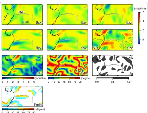
We discuss here the faulting type, the size, and the dip angle of the TNF from the features of the Bouguer anom-alies and the indices derived from the gravity gradient tensor. Around the TNF, the Bouguer anomalies are high on the southeastern side and low in the northwestern side of the TNF, indicating that the basement depth of the southeastern side is shallower than that of the north-western side (Fig. 1). For indices derived from the gravity gradient tensor, high HD (> 2 mGal/km) and high TDX (> 75°) are distributed parallel to the strike of the TNF mainly in the southeastern side of the TNF (Fig. 4). We recognize that VD is high on the southeastern side and low on the northwestern side of the TNF. This difference also indicates that the basement depth of the southeast-ern side is shallower than that of the northwestsoutheast-ern side. Furthermore, the zero isoline of VD, which illustrates a subsurface geological discontinuity, lies parallel to the strike of the TNF mainly in the southeastern side. These features indicate that the TNF is a reverse fault dipping to the southeast. This fault type estimated from the indi-ces is coincident with that based on geological and geo-morphologic observations (Active Fault Research Group
1991; Imaizumi et al. 2018).
The spatial extent of high HD along the TNF is almost identical to that of the surface trace of the TNF reported by Imaizumi et al. (2018) (Fig. 4). The high TDX zone along the TNF is crossed by other high TDX zones with north–south orientation near the coast and at the northeastern extension of the TNF. The zero isoline of VD along the TNF also bends perpendicularly near the coast and at the northeastern extension of the TNF. Low
Di (< 0.5), which indicates that the subsurface
struc-ture is close to two-dimensional one, is distributed over an almost identical range of the total length of the TNF and high Di (> 0.5), which indicates that the subsurface
structure is nearly three-dimensional near both edges of the TNF. We infer from these features that the size of
the subsurface fault structure of the TNF is compara-ble to that of the surface trace. It is also noteworthy that the TNF shows no continuous structure with surround-ing active faults based on the indices calculated from the gravity gradient tensor.
To estimate a fault dip angle, Kusumoto (2016) pro-posed that βmin of a fault structure should be evaluated
in areas with high HD and low Di because a
two-dimen-sional subsurface fault structure satisfies both these con-ditions. Figure 4 shows the distribution of βmin in areas
with HD ≥ 2 mGal/km and Di < 0.5. We took the absolute
value of βmin for use in the plot because we are concerned
about the dip angle. From βmin along the TNF, we can
estimate that the dip angle of the TNF is approximately 45°–60°.
Two‑dimensional density structure analysis
To assess the adequacy of the dip angle estimated from the gravity gradient tensor analysis in Subsect. “Faulting type, continuity and size, and dip of the TNF” section, this subsection presents estimation of the dip angle of the TNF using the 2D Talwani’s method. For calcula-tion, we set the value of the resampled gravity anomaly on the fault trace, at Distance = 0 in Fig. 3a, as 0. Fig-ure 3a compares the observed Bouguer anomalies pro-jected onto the line across the TNF and the resampled ones to the synthetic ones calculated from the optimum subsurface density structure using the 2D Talwani’s method. The optimum parameters, which provide the minimum L2 norm, and those 95% confidence range in the parentheses of Db, Dt, θ, and L are, respectively, 800 m (600–1000 m), 200 m (100–300 m), 55° (40–65°), and 2000 m (1900–2100 m). The calculated Bouguer
Fig. 4 Maps of the six components of gravity gradient tensor and indices (HD, VD, TDX, Di, βmin ) calculated from gravity gradient tensor
components. White lines are active faults. Black lines in the VD (gzz) panel represent the zero isoline of VD. White and dark gray areas, respectively, in
the Di panel indicate that whether the subsurface structure is approximately two-dimensional or three-dimensional. βmin shows the dip angle of the
anomalies well reproduced the resampled ones. We also recognize the tradeoff between the parameters: L and
θ become large and Db becomes small as Dt becomes small, and vice versa. The optimum parameters are essentially sensitive to the assumed density: those for the andesite density of 2200 kg/m3 are Db of 800 m, Dt
of 300 m, θ of 60°, and L of 2000 m and those for the andesite density of 2400 kg/m3 are Db of 900 m, Dt of
100 m, θ of 55°, and L of 2000 m. It is important that a high dip angle is estimated as the optimum parameter irrespective of the assumed density of the andesite.
The optimum dip angle of 55° obtained using the 2D Talwani’s method is coincident with that estimated from the gravity gradient tensor analysis. This result supports not only the estimation of the dip angle of the gravity gradient tensor analysis but also the valid-ity of the estimation of the dip angle of a reverse fault from the minimum eigenvector proposed by Kusumoto (2017). This result also shows that the gravity gradient tensor analysis is as useful as the 2D Talwani’s method for estimating the dip angle of a fault structure and has an advantage of estimating widely the distribution of the dip angle.
Implications for TNF formation processes
The TNF dip angle estimated as explained in the pre-ceding two subsections is high for a reverse fault. We discuss here what this high dip angle means. The 2007 Noto Hanto earthquake (MJMA 6.9) occurred on the
Noto Peninsula about 15 km north of the TNF (Fig. 1). The source mechanism is a reverse fault with right lat-eral slip. Seismic and geodetic analyses indicate the dip angle of the fault plane as 60° (e.g., Hiramatsu et al.
2008; Kato et al. 2008; Sakai et al. 2008). Consequently, the estimated dip angle of the TNF, as a reverse fault with high dip angle, is coincident with that of the 2007 Noto Hanto earthquake. Furthermore, the strike of the TNF, with a northeast to southwest orientation, is the same as that of the 2007 Noto Hanto earthquake. A reverse fault with a high dip angle has been formed by inversion tectonics (e.g., Nakamura 1992). Previous reports have described that some active faults in sea areas around the Noto Peninsula, including the source fault of the 2007 Noto Hanto earthquake, have experi-enced inversion tectonics (Yoshikawa et al. 2002; Kata-gawa et al. 2005; Okamura 2007). In other words, those faults have been formed as normal faults accompanying the opening of the Sea of Japan. They have reactivated as reverse faults by crustal shortening initiated from the late Miocene. Inversion tectonics of this kind were inferred for the 2004 mid–Niigata Prefecture earth-quake, which occurred in a similar tectonic setting in
coastal areas of the Sea of Japan (Kato et al. 2006). In this case also, we infer that the TNF might have experi-enced the inversion tectonics.
Conclusions
We have conducted gravity anomaly and gravity gra-dient tensor analyses around the Togi-gawa Nangan fault (TNF) of the Noto Peninsula, central Japan. Indi-ces such as the first horizontal and vertical derivatives derived from the gravity gradient tensor, as well as Bouguer anomalies, indicate that the TNF is a reverse fault dipping to southeast. We illustrate the subsurface fault structure as an area with a high first horizontal derivative and a low dimensionality index along the TNF. The spatial extent of the area is comparable to the total length of the surface trace of the TNF. We observe no continuity between the TNF and other surrounding active faults. The minimum eigenvectors of the grav-ity gradient tensor indicate the dip angle of the TNF as 45°–60°. Modeling using the 2D Talwani’s method sup-ports this dip angle. Comparison of the dip angle of the TNF to those of the source fault of recent large earth-quakes in/around the Noto Peninsula suggests that the TNF has experienced inversion tectonics.
Supplementary information
Supplementary information accompanies this paper at https ://doi. org/10.1186/s4062 3-019-1088-5.
Additional file 1: Figure S1. Distribution of the gravity measurements points in the sea area west off the Noto Peninsula. Red and gray circles, respectively, are those on the seafloor reported by Ishida et al. (2018) and those reported by Geological Survey of Japan (2013).
Abbreviations
TNF: Togi-gawa Nangan fault; HD: first horizontal derivative; VD: first vertical derivative; GNSS: Global Navigation Satellite System; DEM: digital elevation model; TDX: normalized total horizontal derivative.
Acknowledgements
We used gravity data reported by Yamamoto et al. (2011), Geological Survey of Japan (2013), Geographical Survey Institute (2006), and Ishida et al. (2018). We also used the DEM with a 10 m mesh provided by Geospatial Information Authority of Japan and boring data provided by Hokuriku Geological Informa-tion UtilizaInforma-tion Meeting. All figures were created using Generic Mapping Tools software (Wessel and Smith 1998). Constructive comments from anonymous reviewers are useful to improve the manuscript.
Authors’ contributions
YH and MH designed this study. AS, SI, WK, and MH took gravity measure-ments. YH and AS conducted analyses. YH drafted the manuscript. All authors read and approved the final manuscript.
Funding
The analyses conducted for this study were partly supported by JSPS KAKENHI Grant Number 17K05629.
Availability of data and materials
Competing interests
The authors declare that they have no competing interests.
Author details
1 School of Geosciences and Civil Engineering, College of Science and
Engi-neering, Kanazawa University, Kakuma, Kanazawa, Ishikawa 920-1192, Japan.
2 Hokuriku Electric Power Company, Ushijima 15-1, Toyama, Toyama 930-8686,
Japan.
Received: 1 August 2019 Accepted: 10 October 2019
References
Active Fault Research Group (1991) Active Faults in Japan: sheet map and inventories. University of Tokyo Press, Tokyo (in Japanese)
Beiki M (2013) TSVD analysis of Euler deconvolution to improve estimating magnetic source parameters: an example from the Åsele area, Sweden. J Appl Geophys 90:82–91
Beiki M, Pedersen LB (2010) Eigenvector analysis of gravity gradient tensor to locate geologic bodies. Geophysics 75(6):I37–I49
Cooper GRJ, Cowan DR (2006) Enhancing potential field data using filters based on the local phase. Comput Geosci 32:1585–1591
Geographical Survey Institute (2006) Search of gravity data. http://vldb.gsi. go.jp/sokuc hi/gravi ty/grv_searc h/gravi ty.pl Accessed December 26, 2015. (in Japanese)
Geological Survey of Japan, AIST (Eds.) (2013) Gravity database of Japan DVD Edition, Digital Geoscience Map P-2. Geological Survey of Japan, AIST, Tsukuba
Geological Survey of Japan, AIST (ed.) (2015) Seamless digital geological map of Japan 1: 200,000. May 29, 2015 version. Geological Survey of Japan, AIST, Tsukuba
Hiramatsu Y, Moriya K, Kamiya T, Kato M, Nishimura T (2008) Fault model of the 2007 Noto Hanto earthquake estimated from coseismic deformation obtained by the distribution of littoral organisms and GPS: implication for neotectonics in the northwestern Noto Peninsula. Earth Planets Space 60:903–913. https ://doi.org/10.1186/BF033 52846
Hokuriku Geological Information Utilization Meeting (2019) Hokuriku Geologi-cal Information System. https ://www.hokur iku-jiban .info. Accessed 1 July 2019 (in Japanese)
Honda R, Sawada A, Furuse N, Kudo T, Tanaka T, Hiramatsu Y (2012) Release of gravity database of the Kanazawa University. J Geod Soc Jpn 58(4):153– 160 (in Japanese with English abstract)
Imaizumi T, Miyauchi T, Tsutsumi H, Nakata T (2018) Digital active fault map of Japan. University of Tokyo Press, Tokyo (in Japanese)
Ishida S, Miyamoto S, Yoshida S (2018) The outline of gravity measurement on seafloor in the sea area in front of the Shika nuclear power plant. Electr Power Civil Eng 398:110–114 (in Japanese)
Kaseno Y (1993) Geology of Ishikawa-ken, Japan (with Geological Maps). pp 321, Ishikawa Pref. and Hokuriku Geology Institute (in Japanese)
Katagawa H, Hamada M, Yoshida S, Kadosawa H, Mitsuhashi A, Kono Y, Kinu-gasa Y (2005) Geological development of the west sea area of the Noto Peninsula district in the Neogene Tertiary to Quaternary, central Japan. J Geogr 114:791–810 (in Japanese with English abstract)
Kato A, Sakai S, Hirata N, Kurashimo E, Iidaka T, Iwasaki T, Kanazawa T (2006) Imaging the seismic structure and stress field in the source region of the 2004 mid-Niigata prefecture earthquake: structural zones of weakness and seismogenic stress concentration by ductile flow. J Geophys Res 111:B08308. https ://doi.org/10.1029/2005J B0040 16
Kato A, Sakai S, Iidaka T, Iwasaki T, Kurashimo E, Igarashi T, Hirata N, Kanazawa T, Group for the aftershock observation of the 2007 Noto Hanto Earthquake
(2008) Three-dimensional velocity structure in the source region of the Noto Hanto Earthquake in 2007 imaged by a dense seismic observation. Earth Planets Space 60:105–110. https ://doi.org/10.1186/BF033 52769 Kusumoto S (2015) Estimation of dip angle of fault or structural boundary by
eigenvectors of gravity gradient tensors. Butsuri-Tansa 68(4):277–287 (in Japanese with English abstract)
Kusumoto S (2016) Dip distribution of Oita-Kumamoto tectonic line located in central Kyushu, Japan, estimated by eigenvectors of gravity gradi-ent tensor. Earth Planets Space 68:153. https ://doi.org/10.1186/s4062 3-016-0529-7
Kusumoto S (2017) Eigenvector of gravity gradient tensor for estimating fault dips considering fault type. Prog Earth Planet Sci 4:15. https ://doi. org/10.1186/s4064 5-017-0130-0
Matsumoto N, Hiramatsu Y, Sawada A (2016) Continuity, segmentation and faulting type of active fault zones of the 2016 Kumamoto earthquake inferred from analyses of a gravity gradient tensor. Earth Planets Space 68:167. https ://doi.org/10.1186/s0623 -016-0541-y
Mickus KL, Hinojosa JH (2001) The complete gravity gradient tensor derived from the vertical component of gravity: a Fourier transform technique. J Appl Geophys 46:159–174
Murata Y, Miyakawa A, Komazawa M, Nawa K, Okuma S, Joshima M, Nishimura K, Kishimoto K, Miyazaki T, Shichi R, Honda R, Sawada A (2018) Gravity map of Kanazawa District (Bouguer Anomalies). Gravity Map Series 33, Geological Survey of Japan, AIST
Nakamura K (1992) Inversion tectonics and its structural expression. J Tectonic Res Group Jpn 38:3–45 (in Japanese with English abstract)
Okamura Y (2007) Tectonic evolution and active tectonics of the Noto Penin-sula (Hanto) and its surrounding area. Ann Rep Act Fault Paleoearthq Res 7:197–207 (in Japanese with English abstract)
Pedersen LB, Rasmussen TM (1990) The gradient tensor of potential field anomalies: some implications on data collection and data processing of maps. Geophysics 55(12):1558–1566
Sakai S, Kato A, Iidaka T, Iwasaki T, Kurashimo E, Igarashi T, Hirata N, Kanazawa T, the group for the joint aftershock observation of the 2007 Noto Hanto Earthquake (2008) Highly resolved distribution of aftershocks of the 2007 Noto Hanto Earthquake by a dense seismic observation. Earth Planets Space 60:83–88. https ://doi.org/10.1186/BF033 52765
Sutou H, Kitaguchi Y, Yamamoto K, Kono Y (2004) Gravity anomalies and base-ment structures in southern part of the Noto Peninsula, Japan. J Seismol Soc Jpn 56:363–377
Talwani M, Worzel JL, Landisman M (1959) Rapid gravity computations for two-dimensional bodies with application to the Mendocino Submarine Fracture Zone. J Geophys Res 64:49–59
Wada S, Sawada A, Hiramatsu Y, Matsumoto N, Okada S, Tanaka T, Honda R (2017) Continuity of subsurface fault structure revealed by gravity anom-aly: the eastern boundary fault zone of the Niigata plain, central Japan. Earth Planets Space 69:15. https ://doi.org/10.1186/s4062 3-017-0602-x Wessel P, Smith WHF (1998) New, improved version of the Generic Mapping
Tools released. EOS Trans Am Geophys Union 79(47):579
Yamamoto A, Shichi R, Kudo T (2011) Gravity database of Japan (CD-ROM). Special Publication No. 1. The Earth Watch Safety Net Research Center, Chubu University, Nagoya
Yoshikawa T, Kano K, Yanagisawa Y, Komazawa M, Joshima M, Kikawa E (2002) Geology of the Suzumisaki, Noto-iida and Hōryūzan district. Quadrangle Series, 1:50,000, Geological Survey of Japan, AIST, p 76. (in Japanese with English abstract)
Publisher’s Note