SOME CONSEQUENCES OF SELECTION BY CULLING WHEN THERE IS SUPERIORITY OF HETEROZYGOTES

OF

IS SUPERIORITY OF HETEROZYGOTES

EDWARD POLLAK

Statistical Laboratory, Iowa State University, Ames

Received January 24, 1966

Journal Paper No. J-5200 Iowa Agricultural and Home Economics Experiment Station, Ames. Iowa, Project No. 1505,

supported by National Science Foundation Grant G-18093.

N most of the existing theory of selection the genotypes present in a population

I

are assumed to have constant selective advantages or disadvantages in relation to each other. But a different case was considered by HALDANE (1 961 )

.

He as- sumed that generations do not overlap and that in each generation a proportion C of the males and a proportion c of the females are removed from the population between birth and sexual maturity. If there is natural selection the removal is by death, while if there is artificial selection the removed individuals are those culled by the breeder. In both cases the mathematics is the same, so that for convenience we can say that there is selection by culling.

HALDANE

assumed, in conformity with what usually occurs in animal breeding situations, that C

>

c, so that there is more severe culling among males than among females. For simplicity, only the case in which two genes, A and a, were present was considered. It was assumed that there were at least two distinguishable phenotypes among the three geno- types.

A way in ‘which this selection scheme differs from that usually considered is that the adaptive value of a given genotype is no longer necessarily constant, but may change with the frequency of a gene. For in any generation the worst indi- viduals are culled, and this results in reducing the frequency of the most inferior genotype. It is then possible, after a certain number of generations, for some individuals of another genotype to be culled, although originally all such indi- viduals were allowed to breed.

The problem: HALDANE considered cases in which one of the two genes is dominant or partially dominant to the other. W e shall consider a case of over- dominance in which the genotypic values of A A , Aa and aa individuals are yll, y12 and y Z 2 respectively, where y n a

<

yll

<

y12. In every generation some of the individuals having the lowest genotypic values are culled.

Following HALDANE’S notation, we say that the females in the nth generation produce the gametic array p,A

+

(1 - p m ) a while the males of that generation produce the gametic array g,A

+

(1 - g , ) a. Then if the survivors mate at random the genotypic array at birth in the next generation is

p+AA

+

( p n

+

4, - 2p,q,)Aa

+

(1 - p , ) ( 1 - g,)aa

.

and some A A individuals are culled from the males; (c) all the aa’s and some AA’s are culled from both sexes; (d) all homozygotes and some heterozygotes are culled from the males, but only homozygotes (of both types) are culled from the females; (e) all homozygotes and some heterozygotes are culled from both sexes.

The stage w h r e only aa’s are culled: For any generation n which is in this stage, C I ( 1 - p n ) ( 1

-

q n )

.

Consequently,

Thus for n

>

0 we have

p n ( 2 - c

-

C ) 2 ( l - c ) ( l - C > Pn+i =

and

2 - c -

c

n-l Po +qo

2(1-c)

pn =

[

2(1-c) ( l - C )

1

2 - c-

c

n-l

Po

+ q o

qn=

[

2 ( l - c ) ( l - C )

1

2(1-C)

.

Clearly both p n and qn increase with n, so that no equilibrium can be approached in this stage.

HALDANE

solved for the smallest value of n in ( 1 ) for which

C

t

( 1 -pn) ( 1 -qn)

.

This number was found to be finite and bounded by a small number for large values of C. Thus the population cannot remain for long in this condition.

The second stage: This is defined by the inequalities

~5 ( l - p n ) ( l - q n ) < C s ( l - p n ) ( l - q n ) + p n q n * ( 2 )

Thus, as before,

but now

Since some A A individuals are culled from the males, selection in this sex partially undoes thc cffect of the culling of aa’s from the females. It should thus be possible to have equilibrium frequencies p and q among females and males respectively. If these exist they satisfy

P + Q

P

+

q

-

2Pq

2(1-C)

.

l - q =

p = 2(1-c) ( 5 )

Thus

l - q = P[ll

-

c

-

q ]

SELECTION CULLING

( 6 )

Equations

( 5 )

also imply that

4

( 7 ) 2(1--c) - _-~ 4

1 1 - 2 c *

P

'

1 -

2(1-c) Therefore

92-q [l - - c + ( l - k ) ( l - C ) ]

+

( 1 - 2 c ) ( l - C )

= o

.

(8) The solution is the smaller root of (8). This can be seen as follows. From (2) and (7) we have

( l - d ( 1 - - ) = 4 2 - 2 !7

[--I

l - c q S 1 2 c 1 - 2 c 1-22c 1 -2c

or

q2-2(1 - c ) q + (1 - c ) ( 1 - 2 c ) 2 0

.

1

2

By (7), c

<

- and for these values c ( 1-c)

>

c2. Hence q is no larger than the smaller root 1 - c -

d

m

that can be obtained if the inequality sign is replaced by one designating equality. But (6) and (7) imply, equivalently to

(8), that

4 - c

-3.-

= ( 1-C) (1 -2c) 1 -q

The left hand side of this expression is 0 when q = 0 and increases with q until it assumes its maximum value when q = 1 -

6.

Now

whenever 2c

4

-

2 0. This is satisfied for all c. Therefore q is less than the larger root of (8) and

l-c+ ( 1 -242) ( 1-C) -

q

[ l-c+ ( 1 -2€) ( 1 -C) ]2-4( 1-2€) (1 - C)

L

2 q =

- l-c+ (1+2;c) (1-C)

-q

[ 1-( 1 -2c) (l-C)]2-2c[ 1+ (1-2c) (1- C ) ] +cz -

2

(9) We shall now prove that it is possible for this equilibrium to be stable. Let

P n = p

+

d,,,, and qn q

+

d2,,. Equations ( 3 ) and

(4)

imply that

(10)

E. POLLAK

approximately. In matrix notation these equations may be written

- 1 1

-2(1-c) 2(1-c) 2q-I 2p-I

-

2(1-C) 2(1-C)

-

By a well known theorem in matrix algebra

dn+m Amdn = A"lA1dn

+

AmzA,dn

,

where A, and A, are 2 x 2 matrices that do not depend on n and A1 and A, are the (distinct) roots of the equations

1 - A

1

2 ( 1-c) 2(1-c)

2q-1 2p- 1

2 ( 1-C) 2(1-C) 0 = / A - AI1 =

- A

If both these roots are less than 1 in absolute value then

in which case the equilibrium is stable. The roots of (12) are

I-C+(I-c) (2p-I) + d F C + ( 2 p - l ) (1-~)]"8(p-q) (1-c) (1-C)

A = -

4 ( 1 - ~ ) (1-C) 4(1-C) (1-C)

If c is very small, then by (7) q is approximately equal to p and it follows from (7) and (9) that the roots are approximately

[2p( 1 -c)

-

(C-c) ] &

2p(l-c)-(C-c) A =

4 ( 1 - ~ ) (1-C) 4(1-C) (1-C)

C2

-

C

2(1-c) (1-C) 2(1-C) (1-c) (1-lZC)

i

l -

- -

These roots are both less than 1 in absolute value if

CZ

1 -2c

C+-

<

4(

1-C) ( l - C )

7

4 4

14 8

5

5 5

(1 - 3 c + - c Z ) ( 1 - - c + - c Z ) C < -

If this inequality is satisfied the equilibrium is stable. The third stage: The defining relations are

so that all aa’s and some AA’s are culled from both sexes. In this stage

At equilibrium, if it exists, pn+l = pn = p , q,+l = qn = q and

It follows from ( 1 5 ) and (16) that

!a(

1-c) (1-C) - (C-c) -

c-c

- 1 - c -

q = 2( 1-C) 2 ( 1 - C )

p = l - c - -

l-c

c-c

l-c 2(1-c)

.

To test the stability of this equilibrium we proceed as before and write pn = p

+

d1,n

q n = q + & , n

.

We see from (1 5) that if dl,n and d2,% are small then 2p-I

dz,n 29-1

2(1-c) d l p n + 2 ( l-c)

di,n+i =

2p- 1

d1,n

+

2(1-c)

4%

2g--1 2(1-C)

d z . n + l =

The roots of the equation 2p-1

I

%;I;)

2 ( 1-c)

I

2p--1 - A

~ 2( %-l 1-C) 2(1-C)

are 0 and

29-1

2p-1

+ 2(1-C)

A I =

2( 1-c)

3 3

1--c--c++e

- 8 2

-

l - c - C + C C *

h, is less than 1 if

3 3

- c

+ - c -2&

>

c+c

--cc

2 2

or

1 1

2 2

c(--C)

> - - c

.

1 2

If C

<

-

(19) implies that

1 2

which is satisfied for any c. (19) is also satisfied when C = -

.

We need not consider the case C

>

- 1 because it shall be shown that equilibruim cannot be

E2

reached in this stage f o r such values. The root h1 is positive if

3 3

2 2

- C + - c - 2 2 C c < l , or

3 2

4

’

3 2(1

--e>

C <

3(1

- - e )

and

or

The right hand side of (20) is a decreasing function of C and is thus minimized

when C =

-

Both (20) and (21) are always

satisfied. Thus

and the equilibrium in the third stage is always stable. The fourth and fifth stages: In the fourth stage

1 1

where it assumes the value

-

12.

'

2 '

O < X 1 < 1

C

>

(l-pn) (1-qn)

+

pnqn

>

- c

>

(l-pn) (l-qn). ( 2 2 ) Since only heterozygotes are allowed to reproduce among the males

1 qn+l=-

2 ' But. as in the previous stage,

If the population is still in this stage in the next generation, then

1 -

_{_~}

3 -4c

4 ( 1 - ~ ) 4 - 4 ~

.

pn+z = 1 -

'Therefore there is the equilibrium

1 3 - 4c

q = 2 7 P=- 7

which is clearly stable as long as stage 4 is maintained. In stage 5

C

>

c

>

(l-pn) ( 1 - g n )

+

pnqn

P'Q'.

(24)

(a)

so that only heterozygotes reproduce in both sexes. Thus we have the equilibrium 1

This is stable under the circumstances in which it can arise. jn stage 5. then by (24) and (25) we see that

Values of C and c associated with the four equilibria: If equilibrium is attained

(26)

1

c > c > -

2 '

If there is equilibrium in stage 4, then it follows from ( 2 2 ) and (23) that

3 - 4 c - 1 1

- - > c >

8 ( 1 - ~ ) 2 - 8 ( 1 - ~ )

.

l +

8 ( l - C ) C >

For these values of c

Since f l ( 0 )

<

0, c must be larger than the smallest positive root of f l ( c ) = 0,

f l ( c ) = 8 ~ ( l - ~ ) - 1

>

0

.

1 which is -

2

-

d!!

Thus 4 '

1 1

d2

C > - > C > - -

-

= .1465

.

2 - 2 4

If equilibrium is reached in stage 3, then it is clear from ( 1 4 ) , ( 1 5 ) and ( 1 7 ) that

E. POLLAK

c-c ] = 1 - c - C + 2 2 C c .

= 1 - 2(1--C) [c

+

2( 1-C) 1

Thus

C

I

-

Formulas ( 14) and (1 7), with ( 16), also imply that 2 ’

] Z < c

I-c I-c c-c

[ c + 2(1-C) (1-p) (1-q) =

l--c

=

l--c

and

If we let 6 = C-c, this inequality may be written as

Since fz(0)

<

0 we seek values of 6 less than the smallest positive root of f 2 ( 8 ) = 0, which is

c - c < 2 [ q c ( l - c ) ( l - c ) -c(1-C)]

.

f 2 ( S ) = [I - 2 ~ 1 ’ 6’

4-

~ c ( I - c ) ~ 6 - 4 ~ ( l - ~ ) ~

<

0

.

₍₂₈₎

[ 2 q 4 1 - 4 3 - 1

( 1 -2c) 2

Some values of this root are tabulated below.

c .02 .04 .06 .08 . I O

1-c)2]

.

1

“3

_ - -

.I2 . I 4

e

4

“2 6 .214 .272 .303 .324 .338 .347 .352

-

4

1

d.T

4 2

4 ’

Note that it increases with c and that when c =

-

- -

the limiting value of

C

is

i.

But we have already found that C cannot exceed this value. So, in summary, if equilibrium is reached in stage 3, then

1

q.z

c l - -

-

2 4

[ q 4 1 - 4 3 -&(I -cy]

,

2

c < c +

(1-2c)Z

(29) 1

C I -

2

1 1

q.F

,

- > c > - -

-

2 2 4 ’

1 2

If there is equilibrium in stage G? and C 2

-

; then by

(5)

l - q > p + q - 2 2 ~ 9 ,

1 -2q 2 p(l-2q)

.

Therefore, to avoid contradiction,

q S 2 . 1

Now the defining inequalities of stage 2 imply that c < l - p - q i - p q . Hence we have from ( 5 ) and (7) that

c 5 1 -

e(

I-c)p

+

pq = 1

-

2(1-c) 4+-. q2

1

Since (7) also implies that c

<

-

the derivative of the right hand side of (31) is 2 ’

1 2

Thus the right hand side is minimized when q =

-

.

Hence 1 -

_-

1 -4c

1 -c

1-2c 4(1-2c) 4(1-2c)

C I 1 - p

and

fl(c) = - 8c2

+

8~ - 1 I 0

.

I t follows that c can be no larger than the smaller root of fl(c) = 0, so that

The defining inequalities, (5) and (30) also imply that C I 1 - p - q + 2 p q = 1 - 2 ( 1 - C ) ( l - q )

,

C(l-2(1-q)) 5 1

-

2(1-q)

and

C I 1 (33)

”

1

i f C 2 - 2

1 Turning now to the case in which C

<

-

2 ’ we note that such values of C are consistent with having an equilibrium in stage 3. But we see from (17) that for such an equilibrium

Furthermore, if there is an equilibrium in stage 2, then it follows from (9) that

da

-

I-% - -2 [ l - ~ + (1-2~)(l-C)]

(1-k)

+4(1-%)

----

dC 2 W[l-c+

(1-2C)(1-C)]~-4(1-2c)(l-C)

’

1

which is negative whenever c

<

-

It is not difficult to show that if there were a 2 ’

given c for which there is an equilibrium both in stage 2 and stage 3, then f z (6) = 0, where S = C - c and f z ( S ) is the function defined in (28). Therefore if c is fixed, equilibrium occurs in stage 2 for values of C quite distinct from those implied by stage 3. Hence (129) implies that

1 i f C < -

2

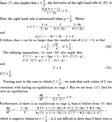
986

FIGURE 1 .-Types

c :

[

;

y

.!io 1.00,

.m

-

C

.W -

.K) 20 30 1 ~ ) 50 60 .m BO .90 100

of equilibria corresponding to proportions culled in

5

of equilibria corresponding to proportions culled in the two sexes.

number below it designates the number of the formula to use for calculating q and p.

How selection by culling can affect the mean genotypic ualue: For simplicity let us consider the limiting case in (which C = c. Stages 2 and

4

are then im- possible, and the relevant equilibrium formulas can be obtained from equations

( 1 7) and ( 2 5 ) . These imply that

1

p = q = l - c , C S 2

1

a '

-

_ -

C > - 1

2 '

If we take r to be the frequency of A among the gametes from which a genera- tion is produced, then the mean genotypic value in this generation is

if there is no selection applied until maturity. This is maximized when r2yll

+

2 r ( 1 - r ) y l Z

+

( 1 - r ) 2 y 2 2 =>(r)

ylz - y z z r =

2y12 - y22 - yll *

,

the population does not have maxi- Thus if I-c differs from

mum mean genotypic value at equilibrium. Indeed it is possible for r ( r ) to actually decline during selection, in spite of the fact that in each generation only individuals having high genotypic values are chosen to reproduce. This is illus- trated by the following example, in which y Z 2 = .40, y l l = .60, y l z = 1 and c = .20. The calculations are summarized below:

ylz - y z z

2Y12 - y22 - yll

n 0 1 2 3 4 5 6 7 8 9 10 CO

r12 .600 .700 .738 .758 .771 .779 .785 ,789 .792 .7W .796 ,800

-

'I'he population is initially in its optimum condition and deteriorates thereafter. One other point that is of interest is that the second derivative of r ( r ) with respect to r is negative. Thus r ( r ) becomes smaller with increasing departure from that value of r which maximizes it. So, if under one intensity of selection, y ( r ) is not maximized when the equilibrium value is attained. it follows that a new equilibrium value of r ( r ) , attained after selection is relaxed, may he even smaller. This would mimic what one would expect to observe if natural selection acted contrary to artificial selection, and there was a relaxation in the artificial selection after equilibrium had been reached. These comments may be relevant to experiments such as that of NORDSKOG and GIESBRECHT (1964), in which a decline in a quantitative character is observed after selection for it is relaxed. T h e calculations of GRIFFING (1960) on selection at two loci also showed that it is not safe to infer from such data that natural selection is operating antagonisti- cally to artificial selection.

_.

DISCUSSION

We have seen that with selection by culling there are always at least two types of stable equilibria when heterozygotes are a t a n advantage. There are four when the proportions of culled individuals differ in the two sexes. It is possible for each of these to be stable, and we have shown that three are always stable.

Another consequence of this type of selection is that the mean genotypic value of the population may actually decline in spite of the fact that individuals with the highest genotypic values are chosen for reproduction in each generation. This can occur if c is too high, because intense selection results in a high proportion of heterozygous parents, which have a high proportion of the inferior aa type of offspring. Thus less intense selection may be better for the population.

One would intuitively feel that in the problem we have discussed individuals having a high genotypic value should be at least as fit in some sense as those possessing a lower genotypic value. This is true if the fitness of a genotype is defined to be the proportion of individuals with the genotype that survive to reproduce. But with selection by culling the average fitness of the population would then be the proportion of the population that survive to reproduce. This does not changeiwith time, while in our example the average performance of the population, measured by

r(

r )

,

actually declines.

time by a continuous variable. To illustrate this, let us consider the genotype Aa. Its fitness is 1 while only homozygotes are being culled and then drops suddenly 1 to a smaller value when culling begins to affect heterozygotes also. If C = c

>

-

2 this value is (l-c)/% or 2 ( 1-c) . The change only takes one generation to be completed, and the new value is maintained afterward.

applicability of the model discussed in this paper to the interpretation of data.

The author wishes to thank PROFESSOR A. W. NORDSKGG for valuable suggestions on the

S U M M A R Y

We have studied a situation in which two alleles at one locus affect a character and the three genotypes are distinguishable. This is not realistic, but may not be very misleading if the distributions of phenotypes associated with the different genotypes differ considerably, at least in their means. Heterozygotes are assumed to be superior in terms of some measurement. Generations are discrete, and selec- tion occurs in each generation by the culling of a proportion of individuals in each sex that have the lowest genotypic values. Survivors mate at random. The culled proportion within one sex is constant from generation to generation but the proportions may differ in the W O sexes. W e have shown that there are four

possible types of stable equilibrium. For a given situation, the type that applies is determined by the proportions culled in the two sexes; there is only one equi- librium for any pair of culling proportions. In addition, selection may result in the decline of the mean genotypic value of the population. This is not consistent with classical selection theory. KIMURA’S generalization of this theory has also been shown not to apply to this case. We have also shown that it is possible in some circumstances for the mean of the population to decline when selection is relaxed. This would mimic the result to be expected if natural selection were operating antagonistically to artificial selection.

LITERATURE CITED

FISHER, R. A., 1930 GRIFFING, B.,, 1960

HALDANE, J. B. S., 1961 KIMUBA, M., 1958

145-1 67.

NORDSKCG, A. W., and F. G. GIESBRECHT, 1964

The Genetical Theory of Natural Selection. Oxford University Press,

Theoretical consequences of truncation selection based on the individual Oxford. Second Edition (1958). Dover Publications, New York.

phenotype. Australian J. Biol. Sci., 13: 309-343.

Some simple systems of artificial selection. J. Genet. 56: 345-350. On the change of population fitness by natural selection. Heredity 12: