The influence of non-classical daming on subsystem response

20th International Conference on Structural Mechanics in Reactor Technology (SMiRT 20) Espoo, Finland, August 9-14, 2009 SMiRT 20-Division 4, Paper 1657

The Influence of non-classical Damping on Subsystem Response

J. Röhner

a

and F.-O. Henkel

a

a

Wölfel Beratende Ingenieure GmbH & Co. KG, Höchberg, Germany, e-mail: [email protected]

Keywords: non-classical damping, state space solution, floor response.

1

INTRODUCTION

Seismic analyses of structures that take into account Soil-Structure-Interaction (SSI) usually result in numerical models that contain different damping ratios for the soil and for the structure itself. Strongly deviating damping characteristics make the model non-classically damped, i.e. after performing a modal transformation the transformed damping matrix will not be diagonal. Ignoring off-diagonal damping terms, as is generally done in a conventional Modal Analysis, may lead to unexpected peaks in response spectra, if the latter are calculated on floors or substructures with natural frequencies close to those of the fundamental modes. This issue, although known for some time, becomes even more important today due to the trend to use the additional speed and capacity that modern computers provide, to develop and analyze very detailed Finite Element models consisting of many vibrating substructures. In the following a 2-DOF system is investigated analytically to gain some insight in the consequences that the diagonal approximation of the transformed damping matrix entails. Subsequently both the 2-DOF and a 3-DOF system are analyzed by conventional Time History Modal Analyses and the results obtained using several common types of damping, are compared with results obtained from a complex modal analysis applying the method of Foss (1958).

2

MODAL ANALYSIS AND NON-CLASSICAL DAMPING

The differential matrix equation governing the response of a viscously damped N-DOF structural system to earthquake ground motions üg(t) is as follows:

) (t ü_g e M v K v C v

M &&+ & + =! (1)

where M, C, K are the mass, viscous damping and stiffness matrix, respectively. The vector v = u - e⋅üg is

the vector of the N-DOF relative displacements and e is the rigid body vector. Dots above symbols denote derivatives with respect to time. The first step in a Modal Analysis is the solution of the free vibration equations:

0

v

K

v

C

v

M

&&

+

&

+

=

(2)

Applying the trial solution

t

e

t ö !

v( )= (3)

yields the Nth order quadratic eigenvalue problem:

0 ö K C

M+ + ) =

(

!

2

!

(4)

Generally the solutions of eqns. (4) are 2N complex eigenvalues and associated complex eigenvectors. As a numerical solution of the free vibration equation requires a linear eigenvalue problem of the form (5) equation (2) must be manipulated accordingly.

0

ö

A

B

!

)

=

(

"

(5)

0 ö M

K! ) =

(

"

* (6)

The solution are N real-valued eigenvalues λn* = ωn 2

and N associated real-valued eigenvectors ϕn which are orthogonal in respect to the mass M and stiffness matrix K. The value ωn is the circular eigenfrequency.

The drawback of the omission of the λC term in the eigenvalue problem (6) becomes evident after transforming eqn. (1) into modal space by setting v(t) = Φ q(t) and pre-multiplying the resulting equation by the transposed modal matrix ΦT:

)

(

t

ü

_g

e

M

Ö

q

K

q

C

q

M

q

Ö

K

Ö

q

Ö

C

Ö

q

Ö

M

Ö

T

&&

+

T

&

+

T

=

&&

+

&

+

=

!

T (7)

While the transformed mass matrix

M

and stiffness matrix

K

are diagonal due to the orthogonality of the

eigenvectors ϕn this is generally not the case for the transformed damping matrix

C

. In order to achieve the diagonal form of

C

, as required by a subsequent modal analysis, the classical types of damping, such as proportional damping (e.g. Rayleigh damping), the diagonal approximation (neglecting off-diagonal terms), composite modal damping (strain energy proportional damping) or the direct assembly of

C

by the specification of modal damping ratios ξn (modal damping) may be applied. However, these types of damping may lead to unexpected results in a conventional modal analysis if different damping characteristics are applied to closely spaced modes.

2.1 2-DOF SYSTEM

Some insight into the phenomenon of non-classical damping can be gained by the following analytical investigation of the 2-DOF system shown in Figure 1. The system mass, stiffness and damping matrices are:

! " # $ % & ' ' + = ! " # $ % & ' ' + = ! " # $ % & = S S S S P S S S S P S P c c c c c k k k k k m m C K M 0 0 (8)

The indices P and S stand for primary and secondary system. Inserting the mass and the stiffness matrix into eqn. (6), and solving the undamped eigenvalue problem, yields the following analytical expression for the circular eigenfrequencies ωn of the coupled 2-DOF system:

(

)

(

1

)

|

1

,

2

4

1

1

2

1

2 2 2 2

2

=

!

+

+

±

+

+

=

""

#

$

%%

&

'

_{! ! !}

n

S n

(

(

µ

(

µ

)

)

(9)

The symbols used in eqn. (9) are µ = mS / mP and χ = ωS / ωP, where ωP = √(kP / mp) and ωS = √(kS / mS) are

the circular eigenfrequencies of the uncoupled primary and secondary SDOF subsystems. In the following ω1

will always be associated to the “+”-sign in eqn. (9) and ω2 to the “-“-sign (i.e. ω1≥ω2). Furthermore the following relations can be deduced from (9):

2 2

2 2 1

1

+

+

!

=

""

#

$

%%

&

'

+

""

#

$

%%

&

'

(

µ

)

)

)

)

S S (10a) 2 2 2 2 2

1

!

!

P

!

S

Figure 1. 2-DOF system Figure 2. Normalized circular frequencies ωn vs. χ, µ = .001

Proceeding in a generic manner and replacing successively λ1* = ω1 2

and λ2* = ω2 2

in eqn. (6), the following eigenvectors can be derived:

2 , 1 | 1 1 2 = ! " ! # $ ! % ! & ' (( ) * ++ , -. /

=a n

S n

n

n

0

0

1

(11)

The factors an were included to facilitate a normalization of the eigenvectors at a later stage. Assembly of the

modal matrix Ö=

[

!₁ !₂

]

and transformation into modal space of the mass and damping matrix yield

M

and

C

, eqn. (7). The non-zero components on the diagonal of the transformed mass matrix

M

are:

2 , 1 | 1 2 2 2 2 = !" ! # $ !% ! & ' + (( ) * ++ , -. /

=a m n

M S n P n nn

µ

0

0

(12)

In order to normalize the eigenvectors in respect to the modal mass matrix, the factors an must satisfy:

2 , 1 | 1 1 2 2 2 2 = !" ! # $ !% ! & ' + (( ) * ++ , -. / = n m a S n P n

µ

0

0

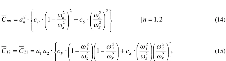
(13)

The diagonal and off-diagonal components of the transformed damping matrix

C

are:

2 , 1 | 1 2 2 2 2 2 2 2 ₌ !" ! # $ !% ! & ' (( ) * ++ , -. + (( ) * ++ , -/ . .

=a c c n

C S n S S n P n nn

0

0

0

0

(14)

!

"

#

$

%

&

''

(

)

**

+

,

''

(

)

**

+

,

-+

''

(

)

**

+

,

.

''

(

)

**

+

,

.

-=

=

2 2 2 2 2 1 2 2 2 2 2 1 2 1 21

12

1

1

S S S S S P

c

c

a

a

C

C

/

/

/

/

/

/

/

/

(15)

Due to the similarity of the system matrices C and K in eqn. (8), the components of the transformed stiffness

By expanding eqn. (15) and using the identities of eqns. (10a) and (10b), it can be shown that in order for the off-diagonal components of the transformed damping matrix to be zero, the viscous damping matrix C must be proportional to the stiffness matrix K:

P S

P S

P S

k k c

c ₌

!

= ₂2

"

"

µ

(16)

or by introducing the damping ratios of the decoupled SDOF subsystems

i i i i

k

c

2

!

"

=

, i = {P, S}:

P S

P S

!

!

"

"

₌

(17)

meaning, that for the tuned system ωP = ωS the damping ratios of the decoupled system must be equal.

2.2

DIAGONAL APPROXIMATION

Proceeding with the classical “diagonal approximation”, i.e. neglecting the off-diagonal terms

0

21

12

=

C

=

C

, to decouple the modal system of equations, the effects of the classical damping type on analysis results of non-classical damped systems can be studied. Normalizing the diagonal modal damping

components Cnnby the modal masses

M

nn and introducing the damping ratios of the coupled 2-DOF

system

nn n

nn n

M C

!

"

2

= , n = 1, 2 yields the following analytical expressions:

2 , 1 |

1 1

2 2 2

2 2 2 2

2 2

, =

+

!! " # $$

% &

'

!! " # $$ % & (

+

!! " # $$

% &

' (

= n

S n

S n

S n

n P

P da n

µ

)

)

)

)

µ

*

+

)

)

)

)

,

,

(18)

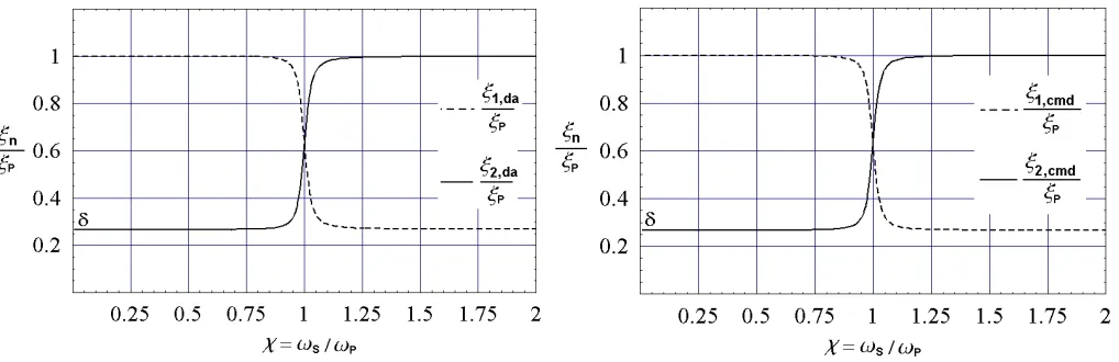
where δ = ξS / ξP is the ratio of the damping ratios of the decoupled subsystems. Applying a mass ratio of µ = mS / mP = 0.001 and “decoupled” damping ratios ξP = 0.15 and ξS = 0.04 to equations (9) and (18) the

normalized circular eigenfrequencies ωn / ωS and damping ratios ξn,da / ξP are displayed over the “decoupled” frequency ratio χ in Figures 2 and 3. As can be seen in Figure 2, as χ passes unity the larger eigenfrequency

ω1 does no longer represent the primary but the secondary system; the opposite can be observed for ω2. The same is true for the associated eigenvectors ϕ1 and ϕ2. A limit analysis of eqn. (9) reveals that:

- as χ→ 0: ω1→ωP and ω2→ωS

- as χ→∝: ω1→ωS (1+µ)0.5 and ω2→ωP (1+µ)-0.5.

The former represents the fully decoupled case, while the latter represents the case where the secondary system is rigidly connected to the primary one.

In modal space this means that for χ≤ 1 the 1st modal equation is associated to the primary subsystem and the 2nd modal equation to the secondary subsystem, while for χ > 1 it is the opposite. This can be seen in Figure 3. A limit analysis of eqn. (18) reveals that:

- as χ→ 0: ξ1,da→ξP and ξ2,da→ξS

- as χ→∝: ξ1,da→ξS (1+µ)0.5 and ξ2,da→ξP (1+µ)-0.5.

damping ratio associated with the primary system is reduced, while the damping ratio of the secondary system increases. This is the reason, why the response of a non-classically damped system shows unexpected behaviour when 2 differently damped modes are nearly tuned and the system is analyzed using classical damping types.

2.3

COMPOSITE MODAL DAMPING

Composite modal damping (strain energy proportional damping) is often used in conventional Modal Analysis when the analyzed system has different damping characteristics. The modal damping ratio of the nth coupled mode is defined by:

(

)

n T n n k i i i T n cmd n

!

!

!

"

!

"

K

K

#

=

=

1 , (19)

where ϕn is the undamped mode shape of the n th

coupled mode and ξi and Ki are the damping ratio and

stiffness matrix of the ith subsystem. Gupta (1999) showed by numerical analysis that composite modal damping is another form of classical damping, as the method also neglects off-diagonal terms in the transformed damping matrix. For the 2-DOF system, equation (19) can be transformed by means of eqns. (11) and (20) into eqn. (21).

(

)

_! " # $ % & ' ' + =

(

= S S S S

S S S S P P k i i i k k k k k

)

)

)

)

)

)

1

K (20)

2 , 1 | 1 1 2 2 2 2 2 2 2 2 2 2 2 2 2 2 , = !! " # $$ % & ' + !! " # $$ % & ( !! " # $$ % & ' + !! " # $$ % & ( = n S n S n S n S n P cmd n

)

)

µ

*

)

)

)

)

µ

*

+

)

)

,

,

(21)

In Figure 4 eqn. (21) is displayed graphically for µ = 0.001. The composite modal damping ratios ξ1,cmd and

ξ2,cmd show the same characteristic behaviour as the diagonal approximation damping ratios. They also change considerably near χ = 1, i.e. when the decoupled subsystems are tuned to each other. Based on these observations, for both composite modal damping and the diagonal approximation a similar response behaviour can be expected.

Figure 3. Normalized damping ratios ξn vs. χ, µ = .001,

”diagonal approximation”

Figure 4. Normalized damping ratios ξn vs. χ, µ = .001,

3

EARTHQUAKE RESPONSE OF NON-CLASSICALLY DAMPED SYSTEMS

The possible effects of non-classical damping on the earthquake response shall be investigated numerically in this chapter. There exist a number of methods that are able to properly account for non-classical damping in a modal analysis, e.g. Veletsos & Ventura (1986), Gupta & Jaw (1985), Igusa et al. (1984) and others. Here Foss’s method was used to calculate the exact solution as comparison to the classical damping solutions.

3.1

FOSS’S METHOD

As in a non-classical damped system the damping matrix C cannot be diagonalized by the transformation given in eqn. (7), Foss (1958) introduced the following 2N x 1 column vectors

! " #

$ % &

= v v z &

! " #

$ % & ' =

g

ü e M

0

f (22)

and 2N x 2N symmetric matrices

! " #

$ % &

=

C M

M 0 R

! " #

$ % &' =

K 0

0 M

P (23)

in order to transform eqn. (1) into:

f

z

P

z

R

&

+

=

(24)

Using a trial solution z(t)=öe"!tand setting f = 0, the following linear eigenvalue problem is obtained:

(

P

!

#

R

)

"

=

0

(25)

The solutions to eqn. (25) are in general 2N complex eigenvalues λn and 2N complex eigenvectors ϕn, the

latter being orthogonal in respect to R and P. Thus a modal decomposition of both matrices is possible and a (complex) modal analysis can be performed. A detailed investigation of this method is given in O’Kelly (1961).

3.2

NUMERICAL ANALYSES

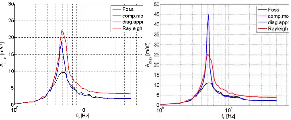
In order to visualize possible effects that may occur in a conventional modal analysis of a non-classically damped system, both a 2-DOF system and a 3-DOF system were analyzed applying the earthquake time history given in Figure 6 and utilizing 3 classical damping types: diagonal approximation, composite modal damping and Rayleigh damping. They are compared to the exact Foss-method.

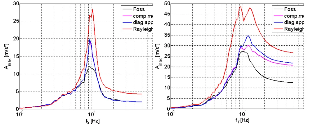
Two sets of system parameters (Figure 5) were applied, the 1st set resulting in the primary and secondary subsystems being detuned in the 3-DOF system analysis and a 2nd set, where the uncoupled eigenfrequencies fP and fS are tuned to 10 Hz. The uncoupled eigenfrequencies of the top subsystems, i.e. fS

of the secondary system in the 2-DOF case and fT of the tertiary system in the 3-DOF case, were varied

Figure 5. 3-DOF system

0 1 2 3 4 5 6 7 8 9 -1.5

-1 -0.5 0 0.5 1 1.5 2

t [s] üg

[ m / s _ ]

Figure 6. Applied acceleration time history

Figure 7a. 2-DOF system 1 – Peak acceleration response

Figure 7b. 3-DOF system 1 – Peak acceleration response

System 1: System 2:

mT = 1 t

ξT = 0.04

fT = ωT /2π (variable)

mS = 10 t

ξS = 0.04

fS = 15 Hz fS = 10 Hz

mP = 10000 t

ξP = 0.15

Figure 8a. 2-DOF system 2 – Peak acceleration response

The following can be observed:

- Rayleigh damping either underestimates or overestimates the response when 2 modes with different damping characteristics are nearly tuned. This is, because Rayleigh damping can only assign one damping ratio for a given eigenfrequency. Here the Rayleigh coefficients were defined based on the values

ξ1 = ξ2 = 0.04 at f1 = 5 Hz and f2 = 15 Hz (f2 = 10 Hz for parameter set 2).

- The diagonal approximation and the composite modal damping result in almost the same maximum response for both the 2-DOF and 3-DOF systems, as already observed in Chapter 2.3.

- The 2-DOF system analyses show that both exceed the exact solution whenever the decoupled eigenfrequency fS = ωS / 2π is nearly tuned to the primary subsystem eigenfrequency fP = ωP / 2π.

- In Figure 7b the acceleration response of the tertiary subsystem is given for parameter set 1, i.e. when the primary and secondary systems are detuned. The peak response occurs when the tertiary system is tuned to the primary system and the peak response predicted by the diagonal approximation and composite modal damping is almost twice as large as the “conservative” Rayleigh values and four times larger than the exact values.

- When the decoupled eigenfrequencies of the primary and secondary subsystems are tuned to each other (Figure 8b) than all classical damping types result in incorrect response predictions for the tertiary subsystem beyond fT≈fP = fS = 10Hz. This is, because the response of the secondary subsystem (Figure

8a) already deviates considerably from the correct solution.

4

CONCLUSION

Non-classically damped systems are common in engineering practice. When analyzed by conventional modal analysis and classical damping types, unexpected results may occur whenever 2 modes with different damping characteristics are nearly tuned. Up to now the compactness of numerical models usually prevents these special cases of tuned modes with different damping. They may be expected more often considering the trend to more detailed structural models, that incorporate a lot of vibrating substructures.

REFERENCES

Foss, K.A. 1958. Co-ordinates which uncouple the equations of motion of damped linear systems. J. Appl. Mech. Vol.25. P 361-364

Gupta, A. 1999. Significance of nonclassical damping in coupled system analysis. Transactions of SmiRT-15. P VIII-257 – VIII-264

Gupta, A.K., Jaw, J.W. 1985. Seismic response of nonclassically damped systems. Nucl. Engrg. Des. Vol. 91, P 153-159.

Igusa, T., Kiureghian, A.D., Sackman, J.L. 1984. Modal decomposition method for stationary response of non-classically damped systems. Earthq. Eng. Struct. Dyn. Vol. 14, P 217-243

O’Kelly, M.E.J. 1961. Normal modes in damped systems. Thesis at the Dynamics Laboratory of the California Inst. of Technology.