Thermal and Non-Thermal Contributions to the X-ray Spectrum of Large Magellanic Cloud Supernova Remnants

(1)

HENDRICK, SEAN P. Thermal and Non-Thermal Contributions to the X-ray Spectrum of Large Magellanic Cloud Supernova Remnants. (Under the direction of Associate Profes-sor Stephen P. Reynolds).

(2)

(3)

by

Sean Patrick Hendrick

A dissertation submitted to the Graduate Faculty of North Carolina State University

in partial satisfaction of the requirements for the Degree of

Doctor of Philosophy

Department of Physics

Raleigh

2003

Approved By:

Dr. Chueng R. Ji Dr. Thomas Drake

(4)

Biography

I was born in Philadelphia, PA on June 14, 1973, son to John Francis and Kathleen Elizabeth, and younger brother to 14 month old Kevin Michael. We moved to the suburbs shortly there after, growing up in Oreland, PA, just outside the city limits. Starting at a very young age, my brother and I participated in organized baseball, basketball, and soccer learning the lessons sportsmanship and teamwork along the way (usually with our father as the coach and our mother in the crowd). A common site in my house would be my father sitting and reading science-fiction novels, a trait I reflect to this day. When I was in the second grade I asked him which of his books I should read; he handed me Isaac Asimov’s “Foundation Trilogy,” and from that moment on I was hooked. In those early years we would pack up for the summer, and move down to Ship Bottom, NJ. I’d spend my days on the beach and my nights looking at the stars. Later, I would spend the summers from 1989–1997 working as a lifeguard for the town of Ship Bottom getting paid to sit on the beach that I loved so much.

After attending public school in Springfield Township (Montgomery County), I attended La Salle College High School in Wyndmoor, PA under the expert tutelage of the Christian Brothers. I was able to academically excel in my years there, as well as participate in a wide range of activities from “Math-letes” to the football team. Besides any academic acheivements, I am quite proud of my years playing football and lifeguarding. The reason for this is that I do not walk as most men do; nerve damage caused my right leg not to grow with the rest of me. As a result it is an inch or two shorter than the left leg, and the foot, three shoe sizes smaller, continues to resist my brain’s attempts to wiggle my toes or move my ankle beyond a small angle. This causes me to walk with a limp that becomes quite painful after an extended period of time. However, I am quite aware of how lucky I am compared to some, and I never let it hold me back.

(5)

(6)

Acknowledgements

I would like to thank my advisor, Stephen P. Reynolds, for his guidance and patience over the years. Also, I could not have completed this dissertation without hours of discussions in Kazimierz J. Borkowski’s office. I thank you for always having your door open, as I have truly enjoyed all our talks.

My data would have been quite useless without the people that work so hard to maintain the software and answer questions at HEASARC and the CXC. Special thanks to Keith Arnaud, Paul P. Plucinsky, and Mike Raley.

I thank all my teachers from La Salle HS, to Virginia, to here at NCSU, for reminding me that there is always more to learn.

(7)

List of Figures

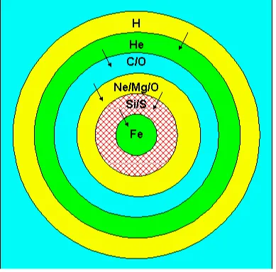
1.1 Structure of a massive star prior to explosion(from Kaler, 1992). . . 10

1.2 Mass transfer between a white dwarf and its companion that results in a Type Ia explosion (image taken from http://www.astro.psu.edu/users/rbc/-a1/lec12a.html). . . 11

1.3 Depiction of the RH jump conditions at the shock front. . . 12

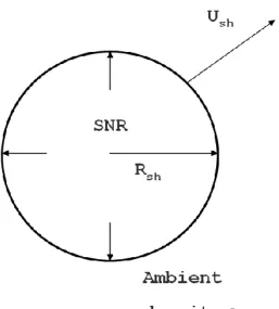
1.4 Sedov phase SNR, an explosion expanding in a uniform medium. . . 13

2.1 Physical process of bremsstrahlung radiation, from the electron’s frame of reference. . . 24

2.2 Physical process that generates synchrotron radiation (taken from http://chan-dra.harvard.edu/resources/illustrations/). . . 25

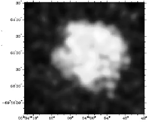
2.3 ROSAT image of SNR 0534-69.9 (from Williams et al., 1999). . . 26

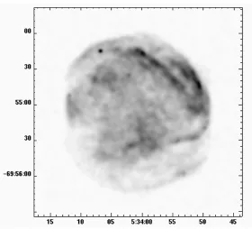
2.4 Chandra image of SNR 0534-69.9. . . 27

3.1 Electron temperature history of solar abundance (crosses), pure oxygen (x’s) and pure iron (asterisks) plasmas for shock with velocity 1000 km s−1. . . . 46

3.2 Electron temperature history of solar abundance (crosses), pure oxygen (x’s) plasmas scaled to maximum solar T_e. . . 47

3.3 Electron temperature history of solar abundance (crosses), and pure iron (x’s) plasmas scaled to maximum solar T_e. . . 48

3.4 T_e versus τ plot for values of β = 0.0, 0.1 0.5, and 1.0 (lowest to highest curves). . . 49

3.5 HE shock versusvneifor a pure oxygen plasma. . . 50

3.6 HE shock versusvneifor a pure iron plasma. . . 51

3.7 HE shock versusvneifor a solar abundance plasma. . . 52

3.8 HE shock versusvneifor a pure oxygen plasma, with τ_min = 1×1013 cm−3s. 53 3.9 HE shock versusvneifor a pure iron plasma, with τ_min= 1×1013 cm−3s. . 54

3.10 HE shock versus vnei for a solar abundance plasma, with τ_min = 1×1013 cm−3s. . . 55

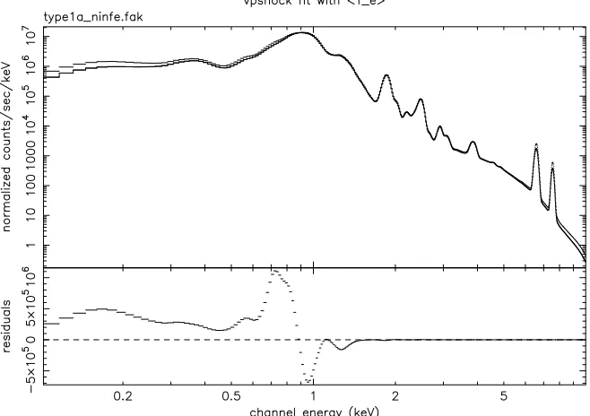
3.11 HE shock versusvpshock for a Type Ia abundance plasma. . . 56

(11)

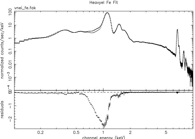
3.13 Evolution of HE shock model predicted spectra for 4 levels of ionization timescale. Lower curve is for τ = 1010 cm−3s, with successive orders of

magnitude up to 1013 cm−3s. . . 58

4.1 Fitted spectrum of N63A with combined SIS0 and SIS1 data. The synchro-tron component is the curve with lower values at lower X-ray energies. . . . 71

4.2 Fitted spectrum of N132D with combined SIS0 and SIS1 data. The synchro-tron component is the curve with lower values at lower X-ray energies. . . . 72

5.1 Image of 0548-70.4, with regions from Hendrick et al. (2003). . . 89

5.2 Same as Figure 5.1, with the NW and SE regions and the central region halves. 90 5.3 Sedov model fit to West limb spectrum. . . 91

5.4 Sedov model fit to East limb spectrum. . . 92

5.5 Comparison of Central region to the East limb (circles). . . 93

5.6 Two-component vpshockfit to Center . . . 94

5.7 Two-component HE shock fit to Center . . . 95

5.8 Comparison of the Central region to EC (circles) and WC (squares) halves. 96 5.9 Comparison of the NW region and the West limb (circles). . . 97

5.10 Two-componentvpshockfit to the NW limb . . . 98

6.1 Image of 0534-69.9, with NW, S, and E limb regions. . . 109

6.2 NW region of 0534-69.9 behind the limb. Note the detailed morphology. . . 110

6.3 Same as Figure 6.1, with NE, S, NW, and SE central regions. . . 111

6.4 Sedov model fit to the NW limb spectrum. . . 112

6.5 Spectral comparison of the NW, S (squares), and E limb (circles) regions. . 113

6.6 Sedov model fit to the W loop region. . . 114

6.7 Two-component vpshockfit to NE center . . . 115

6.8 Two-component HE shock fit to S center . . . 116

6.9 Two-component vpshockfit to NW center . . . 117

6.10 Two-componentvpshockfit to SE center . . . 118

7.1 Smoothed image of 0453-68.5, with regions drawn for the E, NW, and S limbs. The interior regions represent the NW horizontal and NW vertical components. . . 129

7.2 On the left, the soft band (0.3-2.0 keV) smoothed image of 0453-68.5, com-pared to the hard band (2.0-8.0 keV) on the right. . . 130

7.3 Spectral tomography maps between 20 cm and 13 cm radio emission. . . 131

7.4 2D fit results to the PWN image. . . 132

7.5 Sedov model fit to the NW limb . . . 133

7.6 Spectra of the three limb regions: NW, E (boxes), and S (circles). . . 134

7.7 Comparison of radio (left) and X-ray (right) emission. . . 135

7.8 Spectral comparison of the S limb and the SW region (boxes). . . 136

(12)

(13)

List of Tables

2.1 X-ray line emission in keV (Bearden, 1967) for neutral atoms . . . 28

3.1 NEI fits to HE shock model . . . 59

3.2 SN ejecta abundances from Iwamoto et al. (1999) normalized to Fe . . . 60

4.1 Radio parameters for LMC supernova remnants . . . 73

4.2 Summary of X-ray observations . . . 74

4.3 Rolloff frequencies and energy upper limits . . . 75

4.4 Rolloff frequency dependence on radio parameters for DEM L71 . . . 76

4.5 Rolloff frequency dependence on radio parameters for N63A . . . 77

5.1 Sedov model fits to limb regions of 0548-70.4 . . . 99

5.2 Two-component fits to central regions (EM units are cm−5) . . . 100

5.3 Fit summary of NW limb region . . . 101

6.1 Sedov model fits to limb regions . . . 119

6.2 Sedov model fits to NW regions . . . 120

6.3 Two-component fits to NE and S central regions . . . 121

6.4 Two-component fits to SE and NW central regions . . . 122

7.1 Sedov model fits to limbs . . . 139

(14)

Chapter 1

Supernovae and Their Remnants:

An Overview

1.1 What Is a Supernova?

When a main sequence star runs out of hydrogen fuel in its core, it starts on the path to its final state. Our Sun will expand to a red giant (to the orbit of Venus, about 200 times its current radius) as the helium core shrinks due to gravity and a thin hydrogen burning shell about the core expands. Helium burning will begin in the core creating carbon and oxygen. When the helium burning in the core is exhausted the star will eject its outer H and He burning layers and leave behind a white dwarf (about the size of the Earth). Solitary white dwarf stars slowly cool from 105 K to thermodynamic equilibrium with the surrounding space. More massive stars die in violent explosions known as supernovae. It is in these supernova explosions that the heavy elements of the periodic table are formed and dispersed throughout the interstellar medium (ISM). The stellar lifecycle is continued as new star formation begins due to the injection of energy and material into the ISM.

(15)

of the explosion appeared as a bright ‘guest star’ that disappeared after a few months, with some so bright they were visible during the day. The optical spectra observed for supernovae distinguish between the types of explosion by the presence of hydrogen lines. Type II explosions have H-lines, Type I explosions do not. The energy source of the bright optical signal is the radioactive decay of nickel to cobalt (6.1 day half-life) and then cobalt to iron (77.1 day half-life). Once that is complete, the optical signal fades away. Type I explosions are further classified as Ia, Ib, and Ic based on their spectra. Type Ia explosions contain silicon lines, Ib and Ic do not. Type Ib explosions are helium rich, while type Ic supernovae are helium poor. For each type of explosion, about 1051 ergs of kinetic energy is inferred to be carried into the ISM. A review of supernova explosions and their optical signals can be found in Kirshner (1988).

1.1.1 Type II

(16)

1.1.2 Types Ib and Ic

The explosion mechanism in Types Ib and Ic is the same as for Type II, the gravitational collapse of a massive star as seen in Figure 1.1. The difference is that the outermost layers of the star have been lost prior to the explosion. For Type Ib, the star has released its hydrogen layer in its stellar wind. Type Ic explosions lack both H and He lines indicating the loss of the two outermost layers. As above, neutron stars, and possibly black holes, are formed as a result of Type Ib and Ic explosions.

1.1.3 Type Ia

Type Ia explosions are from white dwarf stars in binary pairs. White dwarfs are very dense, almost the mass of the Sun condensed to the size of the Earth. When their companions expand to become giants the white dwarfs can tug on their outer layers. Mass transfer occurs through an accretion disk to the white dwarf from its companion, as seen in Figure 6.2 (image taken from http://www.astro.psu.edu/users/rbc/a1/lec12a.html). This will eventually push the star over the 1.4M_¯ Chandrasekhar mass limit. The quantum effect of electron degeneracy pressure can no longer maintain the star, and deflagration (subsonic burning) of the carbon and oxygen results in an explosion, totally destroying the star. 1.4M_¯of material, larger iron, is ejected at 10,000 km/s, releasing 1051 ergs in kinetic energy, but there is no corresponding neutrino flux.

1.2 Astrophysical Shocks

Each explosion creates a shock wave, a disturbance moving into the surrounding medium highly supersonically. These blast waves propagate into the ISM heating particles, sweeping them along, compressing magnetic fields, destroying dust, crushing interstellar clouds, and accelerating cosmic rays. A shock can be approximated as a discontinuous jump when the mean free path of the particle is much less than the macroscopic length scale. At the jump, the Rankine-Hugoniot jump conditions apply (Shu, 1992, equations 15.31-15.33):

(17)

ρ₂u2₂+P₂ =ρ₁u2₁+P₁ (1.2)

1 2u

2

2+h2 = 1 2u

2

1+h1 (1.3)

h= γ

γ−1

P

ρ (1.4)

where the subscripts indicate upstream (1) and downstream (2) in the shock frame, and h

is specific enthalpy. We shall assume a monatomic gas with γ = 5/3. A basic picture of a shock front is found in Figure 1.3. Cold, rarefied material is upstream from the shock, and as the shock passes it becomes hot and dense. The ideal gas law can relate temperature to pressure.

P = 3 4ρ2v

2

s =k(ne+ni)Ts (1.5) The pressure term is the ram pressure generated by a shock with speedv_sin the downstream region. A shock at 10,000 km/s heats the plasma to temperatures above 107 K. The thermal radiation of the particles extends to the X-ray regime at these temperatures. We assume a shock to be ‘collisionless,’ with no Coulomb collisions at the shock front and magnetic fields mediating the particle interactions. This is a good approximation when the Coulomb mean free path is much greater than the gyroradius of the thermal particles.

(18)

Another important issue is the creation of a reverse shock. The blast wave travels out to the ISM, driven by the material ejected from the progenitor star. At the interface between the ISM and the ejecta, a reverse shock can form once the outer shock has slowed significantly. This shock will travel backwards, in the Lagrangian frame, through the ejecta that have enhanced abundances of heavy elements from stellar fusion processes. Dwarkadas & Chevalier (1998) calculate how long the reverse shock will travel through the ejecta before reaching the center and dissipating. In Chapters 5 and 6 we will examine how to distinguish between the ejecta heated by the reverse shock and the ISM material heated by the forward shock.

1.3 Supernova Remnants

Possible stellar remnants of a supernova are a black hole, a neutron star, or nothing. In each case, a supernova remnant (SNR) is formed by the expanding shock wave after the explosion, once it has had time to interact with the ISM and ejecta. As more material is swept up by the shock, it decelerates, eventually dissipating over a few 105 −106 years. SNR evolution consists of three stages.

1.3.1 Ejecta Dominated

In the early stage, the freely expanding ejecta dominate the dynamics of the rem-nant. The reverse shock is prominent, and the ejected mass is greater than or comparable to the ISM mass swept up by the forward shock. The X-ray spectrum will indicate the elemental abundances of the ejecta as well as the ISM. This stage lasts for the first few thousand years of the remnant’s life. Examples of ejecta dominated SNRs are Galactic remnant Cassiopeia A, Small Magellanic Cloud (SMC) remnant 1E0102-72.3, and the very young Large Magellanic Cloud (LMC) remnant SN1987A.

1.3.2 Sedov Phase

(19)

(Sedov, 1959). Figure 1.4 is the picture of a strong shock wave expanding in a uniform medium. Now the X-ray spectrum is indicative of the shocked ISM abundances. The Sedov solution assumes an explosion in a uniform medium of density ρ with energy E. The following equations describe the evolution of the SNR radiusR and shock speedv_s as functions of time (assuming tha adiabatic indexγ = 5/3):

U_sh= 2 5

R

t (1.6)

R = 1.15 µ

E ρ

¶₁_/₅

t2/5 (1.7)

whereU_sh is the speed of the forward shock propagating into the ISM. General age ranges for the Sedov phase are 10,000 to 100,000 years after the explosion. Examples of Sedov phase remnant include the LMC remnants 0548-70.4, 0534-69.9, and 0453-68.5 discussed in this work.

1.3.3 Radiative Phase

Known as the ‘snowplow’ phase of SNR evolution, this begins when the shock temperature drops below 106 K. Radiative cooling becomes important, and the shocked material becomes too cool to be observed in X-rays. The forward shock will continue to sweep up ISM material as momentum conservation takes over the dynamics. Eventually the material will become fully mixed into the ISM, and will be incorporated into the next generation of stars.

These three stages of SNR evolution are oversimplified. Transitions between the stages are gradual, and parts of a remnant can be in radiative phase even when global remnant dynamics are still based on the Sedov phase. Likewise, remnants entering the Sedov phase can still contain significant emission from ejecta in the SNR interior.

1.4 Interstellar Medium

(20)

conditions of the ISM will affect the morphology of the SNR since the shock front will slow down in denser material. Understanding the composition of the ISM near a remnant is an important issue. Spitzer (1978) Chapter 1 gives an excellent review of the components of the ISM. The state of interstellar gas can be defined in terms of temperature:

• Molecular gas – at very low temperatures, T ∼ 10 K, simple molecules such as H₂

and CO can form. Such clouds are nearly opaque.

• Atomic gas – hydrogen is the most abundant element in the universe, and large amounts exist between the stars. At temperatures of T ∼ 100 K neutral hydrogen and helium make up a majority of the ISM mass.

• Ionized gas – stars that are strong sources of ultraviolet radiation can provide the 13.6 eV necessary to ionize hydrogen. Ionized nitrogen and oxygen are also observed around the young O and B type stars with high surface temperatures of T∼10,000 K that photoionize the gas. Higher levels of ionization occur in collisionally ionized gas where temperatures of 107 K are generated by a shock wave.

Besides gas, we must consider two other important constituents: dust and magnetic fields. Dust grains with radii smaller than 10−4 cm have a strong effect on observations. They are composed of graphite, iron, silicon carbide, silicates, and frozen gas. Dust scatters and absorbs light of all wavelength, with increasing effects against decreasing wavelengths. Interstellar magnetic fields align these grains and polarize the light from objects we attempt to observe through them. The field strength in the ISM fluctuates over both large and small scales, with a mean value ofB∼3µG. Magnetic fields are also responsible for synchrotron radiation when interacting with relativistic electrons in the galactic plane.

(21)

neutral hydrogen that are very common. They have temperatures of T∼100 K, and contain 10-100 M_¯ at densities of ∼20 cm−3. When these clouds exist near, or surrounding, hot O and B type stars, parts of the HI cloud become photoionized HII regions as described above. Molecular clouds make up the other form of the cold ISM. With low temperatures of T∼10 K, and densities ranging from 10-1000 cm−3, or higher, simple molecules can form. Within giant molecular clouds, R ∼100 pc, gravity and magnetic fields mediate new star formation.

Evolution of the ISM is dependent on supernova explosion. New explosions send energy and material to the ISM. Existing clouds are heated and crushed, and new clouds form as the thin dense shells of the hot phase cool down. The components are in rough pressure balance with one another (n₁T₁ ∼ n₂T₂), and they mix and cool to create new stars. It is the inhomogeneity of the ISM within the Galaxy that makes observing local supernova explosions difficult. A general estimate of SN explosion rates predict 1 event each 20 years (Heiles, 1987), and yet the explosion observed by Kepler in 1604 is the last recorded in our Galaxy. This discrepency is most likely a result of the ISM obscuring events from our view. There is little material between galaxies, so we can turn to the Magellanic Clouds for a full sample of supernovas. There we can observe SNRs interacting with the local ISM with little absorption along our line of sight.

1.5 Broadband Detection of Supernova Remnants

After the initial light from the explosion, the expanding remnant radiates through-out the entire electromagnetic spectrum. In the radio regime, synchrotron radiation from relativistic electrons (energies∼1−10 GeV) spiraling in magnetic fields is prominent. The combination of high-energy particles and compressed magnetic fields make most supernova remnants very bright in radio. The possible presence of a neutron star acting as a pulsar can also be determined by radio observations.

Infrared observations indicate the thermal emission from dust that is heated and destroyed by the shock and newly created dust in the wake of the shock wave. The visible spectrum contains emission from collisionally ionized atoms (SII, NII, OIII, etc) and Hα

(22)

explosion, the shock wave ionizes the neutral H in the ISM to create the Balmer emission. Ultraviolet observations of SNRs show emission from higher ionized states than in the optical, indicating hotter material that is cooling down to optical levels.

This work will concentrate on X-ray observations of SNRs. The highly ionized states created by the shock include hydrogen-like ions of C, N, and O, and helium-like ions of Si, S, and Fe. L-shell and K-shell line emission are observed for heavy elements. There is also a continuum component in the X-ray regime that contributes to the spectrum. Chapter 2 reviews the details of each type of X-ray emission. The ionization stages observed in ultraviolet and optical occur as the metals cool from these X-ray states with post-shock temperatures of 107K. Besides the emission from hot thermal gas, there is some indication of SNRs with non-thermal tails in the hard X-ray regime. With the X-ray observatories placed in orbit over the past 30 years, our understanding of supernova remnants has increased with each new detector. Data sets from both the ASCA and Chandra satellites are analyzed herein.

1.6 Summary

(23)

(24)

(25)

(26)

(27)

Chapter 2

X-ray Spectrum: Emission,

Detection, and Analysis

2.1 Introduction

(28)

2.2 Radiative Processes

2.2.1 Bremsstrahlung

Bremsstrahlung, or braking radiation, is the energy loss of electrons accelerated in the electric fields of passing nuclei. This form of radiation was orginally discovered as the explanation for decelerating beams of electrons. This process is identical to free-free emission of an electron making the transition between unbound states of the nucleus. Similar nonrelativistic particles (electron-electron, or proton-proton) exhibit no radiation of this form. It is in the interaction between electrons and ions that bremsstrahlung occurs. Thermal bremsstrahlung indicates a Maxwellian distribution of electron velocity, while non-thermal bremsstrahlung implies a non-Maxwellian distribution, and depends on knowing the actual velocity distributions. There is also the case of relativistic bremsstrahlung. Electrons with energy below 1 MeV are non-relativistic and ionization losses are important. Above 1 MeV is the relativistic regime when relativistic bremsstrahlung losses dominate. Excellent summaries on bremsstrahlung can be found in Longair (1992) chapter 3, Rybicki & Lightman (1979) chapter 5, and Shu (1991) chapter 15.

Figure 2.1 shows an electron moving at velocityvpast an ion of charge Ze, whereb

is the impact parameter. The electrostatic force ofF =Ze2/4π²₀b2 is experienced between the electron and nucleus, for a duration of 2b/v. The momentum impulse of this force translates into kinetic energy transfer between the particles. Impulse perpendicular to the electron’s velocity is the dominant contributor to the radiation. We must determine the number of collisions within a range of impact parameters to examine the radiation spectrum. From the electron’s frame of reference, we get the following equation (Longair, 1992, equation 3.35):

I(ω) = Z2e6N 12π3²3₀c3m2_e

1

vln b_max

b_min (2.1)

(29)

defined as γv/ω, the limit when radiation is in the exponential tail and doesn’t contribute to the intensity. b_min can be calculated in the classical limit for low velocity electrons (Ze2m_ev2/8π²₀), or in the quantum limit for fast electrons (~/2m_ev). The logarithm of

b_max/b_min is also known as the Coulomb logarithm, ln Λ.

The equation above is for a single electron. We must include a Maxwellian dis-tribution of velocities for the electrons as appropriate for a thermal plamsa. For thermal bremsstrahlung the spectral emissivity (radiated power per unit volume and frequency) is (Longair, 1992, equation 3.43):

K_ν = 6.8×10−51Z2T−1/2N N_eexp(−hν kT) Wm

−3_Hz−1 _(2.2)

This equation demonstrates the exponential drop off of bremsstrahlung radiation due to the low numbers of electrons available in the high velocity portion of the Maxwellian distribu-tion. The energy loss rate for bremsstrahlung is (Longair, 1992, equation 2.45):

−dE

dt = 1.435×10

−40_T1/2_Z2_{N N}

e¯g Wm−3 (2.3)

The ¯g term is the Gaunt factor, defined as the Coulomb logarithm averaged over velocity and frequency (for hν¿kT, ¯g∝ν−0.1). For a Maxwellian distribution, this factor ranges in value from 1.1-1.5 for most plasma conditions. The spectrum of the radiation is roughly flat up to hν∼kT, above which it begins to drop off. Non-thermal bremsstrahlung needs a new calculation of gaunt factors as well as knowledge of the velocity distribution. For relativistic bremsstrahlung, a correction factor must be added to the equations to account for the new values ofb_maxandb_mincalculated in the relativistic limit. This work will employ non-relativistic thermal bremsstrahlung to define the continuum emission found in SNRs, since most electrons in SNRs have energies far below 1 MeV.

2.2.2 Synchrotron

(30)

andmc→γmcinω_B. The electric field of the electrons, which varied sinusoidally with the same frequecy ω_B as the gyration in the magnetic field, becomes a series of sharp pulses, repeating for time intervals of 2π/ω_B, as velocityv→c. The spectrum now involves many harmonics at integer multiples ofω_B/γ, up to a maximum frequency ofγ2ω_B/2π. A power law distribution in electron energy creates the power law spectrum observed. This spectrum is the Fourier transform of the sharp pulses in the electric field. Relativistic electrons create time dilation effects in arrival time of the radiation from different points in its orbit, and we must also consider the Doppler shift in frequency. For a single electron, the power per unit frequency is found to be (Rybicki & Lightman, 1979, equation 6.18):

P(ω) =

√

3 2π

e3Bsinα mc2 F

µ

ω ω_c

¶

(2.4) whereF(ω/ω_c) is a dimensionless function defined in Longair (1994) Table 18.1. The critical frequency above is defined as ω_c = (3/2)γ3ω_Bsinα, where α is the pitch angle between the magnetic field and the velocity of the electron. At low frequencies this term rises as (ω/ω_c)1/3, peaking at ω/ω_c = 0.25, and then drops off exponentially for high frequencies

ωÀω_c.

With multiple electrons, distribution in position will create different angles with the B field. Each electron will therefore have slightly different harmonic values. Distribution in electron energy will add further broadening of the lines that creates the continuum spectrum known as synchrotron radiation. Polarization lets us examine the direction of the magnetic field generating the emission. The motion of the relativistic electrons causes the signal to be beamed in the direction of motion. From a distribution of electrons, we see mainly partial linear polarization, in the direction perpendicular to the projection of the magnetic field on the plane of the sky. For power-law energy distributions of electrons in a uniform magnetic field, the maximum polarized fraction is about 70%, and less in more realistic inhomogeneous situations. The fractional circular polarizationis of order 1/γwhich is normally negligible for radio and higher frequency synchrotron emission in which we infer

γ of order 104 or higher.

(31)

P_tot(ω)∝ω−(p−1)/2 (2.5) where p is the particle distribution index, N(E) ∝ E−p, and the spectral index of syn-chrotron radiation is α = (p−1)/2. The spectrum rises as ω → 0.29ω_c, and drops off exponentially above that value. Synchrotron emission is dominate in the radio regime, but the power law aspect of the spectrum means the effects should continue into the X-ray regime. This depends on how far the electron distribution extends in energy, which consti-tutes a possible test of electron acceleration. In the next chapters, we shall examine how different loss mechanisms cause synchrotron emission to eventually drop off to the levels observed in the X-ray spectrum of the supernova remnants that accelerate the electrons.

2.2.3 Line Emission

Line emission occurs when an electron bound to an atom drops from a high energy level down to a lower energy level and a photon is released. This is the type of emission that is common in neon signs, although much more energy is required for the line to appear as X-ray photons. Each ionization state of each element has unique energy levels that create unique spectra. Line emission observed in the visible regime is caused by transitions between the lower electron levels in nearly neutral atoms. Upper level electrons that drop down to the lowest levels are responsible for X-ray line emission. In a hot plasma, most elements are highly ionized, to H- or He-like states. When these ions collide with an electron, a bound electron can be excited out of the lowest energy levels in atom. This creates a hole in the lower level, usually the K-shell or L-shell, that is filled in by an electron from an upper level. Table 2.1 lists the major lines seen in X-ray spectra for some of the most abundant elements (Bearden, 1967). The strength of the line in a spectrum is proportional to the abundance of that element in the plasma. SNRs have varying amounts of this line emission that can be used to determine the chemical composition of the radiating plasma.

2.2.4 Inverse Compton Scattering

(32)

electron to high energies. Now it is the electron that transfers energy and momentum to the photon. The energy loss rate for a single electron is given by Longair (1992) equation 4.31:

−dE

dt =

4

3σTcUrad µ

v2 c2

¶

γ2 (2.6)

U_rad is the energy density of the photons incident on the electron and σ_T is the Thomson cross-section. This is similar to the energy loss rate for synchrotron radition

−dE

dt =

4 3σTcUB

µ

v2 c2

¶

γ2 (2.7)

with U_B as the magnetic energy density. This is an interesting parallel between radiative processes. With a power law distribution of electrons, we get a power law photon spectrum (no matter what the original photon spectrum was), with the same spectral index as for synchrotron radiation, α= (p−1)/2.

2.3 X-ray Satellites

Observation in the X-ray regime is a purely satellite based field due to photoelectric absorption of X-ray photons in the atmosphere by molecules and atoms. Even with the satellite in orbit, the issue of capturing the high-energy X-ray photons with a telescope remains. Lenses and mirrors used for optical observation are useless for capturing such high energy photons. However, for sufficiently large angles of incidence, an X-ray photon will reflect off a conducting material. A paraboloid surface is effective, but for 1 keV photons only a small range of angles is focused, with the range decreasing as energy increases. Adding a hyperboloid surface after the parboloid shortens the focal length and focuses photons in an annulus defined by the surfaces. Nesting paraboloid-hyperboloid surfaces within each other increases the effective area of the telescope. Once we have collected the signal, unwanted events such as cosmic rays, gamma rays, and high-energy electrons released from the walls of the detector by a cosmic ray must be discerned from the X-ray photons. The isotropic cosmic X-ray background adds even more noise to any observation.

(33)

photons and high energy particles, is usually surrounded by another detector that is only sensitive to particles. Therefore, any event that activates both detectors is flagged for re-moval in processing as a particle event. Within the gas, electron-ion pairs are created. A single pair is created through photoionization by an X-ray photon, while many pairs are created through ionization losses of an energetic particle. With the proper voltage across the gas filled counter, the single electron created by photoionization ionizes other atoms, creating one additional pair for each 30 eV of the incident photon energy. Therefore, the strength of the pulse created is proportional to the energy of the incident photon. Position can be determined by the ratio of the charge at each end of the anode and by using multiple anode wires.

Solid-state detectors improve on the statistical accuracy of gas filled detectors. In this case, electron-hole pairs are created in the material (usually silicon) which needs only ∼3 eV to create a hole. A detector chip consists of sensitive strips separated by thin channel stops. Those strips are further broken up into pixels, each connected to three read-out electrodes. A detector is an array of several hundred of these pixels that allow spatial position of the photons to be recorded. By creating high resistance across a pixel, the holes are pulled into the substrate material while the electrons liberated by photoionization are trapped in the potential well of the pixel. Charge coupled devices (CCDs) are the most widely used detectors on the current missions. Charge coupling refers to the method of reading out the charge by changing the voltage on the read-out electrodes that shifts the charge to the next channel. This process continues across the device until the charge reaches an amplifier which records the charge of each pixel into memory. The efficiency at which the charge is transferred is a very important issue that must be addressed when working with CCD data. The charge contained in each pixel is proportional to the X-ray flux density at that position. Longair (1992) contains an excellent review of all these telescope related issues.

2.3.1 Historical Notes

(34)

mission was the Einstein X-ray Observatory in 1978 (Giacconi et al., 1979), which had five instruments. The most notable of these was the High Resolution Imaging Telescope (HRI). This instrument employed grazing incident optics to increase angular resolution to 4 arcsec with a field of view 25 arcmin in diameter. Deep surveys of small areas led to the discovery of discrete X-ray sources in the Andromeda Galaxy (M31) and the Magellanic Clouds. In 1990, ROSAT (Truemper, 1982) was launched to perform a survey of the entire sky in soft X-rays. The catalog created by the ROSAT All-Sky Survey (RASS) is still used for the planning of new observations. It was 1000 times more sensitive than UHURU and discovered 150,000 objects. It also discovered the detailed morphology of SNRs in X-rays.

2.3.2 ASCA

The Advanced Satellite for Cosmology and Astrophysics (ASCA) was launched in 1993 and operated for seven and a half years (see Tanaka et al., 1994). Archival ASCA datasets were used in Chapter 4 of this work to examine 11 supernova remnants. It was the first X-ray telescope to use CCDs among its four instruments. ASCA contained two gas imaging spectrometers (GIS2 and GIS3) that contained imaging gas scintillation pro-portional counters, and two solid-state imaging spectrometers (SIS0 and SIS1). 120 nested gold-coated aluminum foil surfaces in the telescope were able to attain an angular resolution of 0.5 arcmin in each detector. Both ROSAT and Einstein HRI detectors had higher spatial resolution, but the strength of ASCA was the high spectral resolution. The CCD devices were sensitive between 0.4-12.0 keV with an energy resolution of about 2% at 5.9 keV, while the GIS could detect between 0.8-12.0 keV, with slightly poorer energy resolution of 8%. ASCA discovered non-thermal X-rays from the Galactic remnant SN 1006, providing a link between the cosmic rays accelerated in that remnant (Koyama et al., 1995) and non-thermal X-rays that is explored in Chapter 4. It could also probe the chemical abundances within distant objects, determining that clusters of galaxies contained material consistent with origin from Type II supernova explosions (Loewenstein et al., 1994).

2.3.3 _Chandra

(35)

Chapter 1. Launched in 1999, theChandraX-ray Observatory has the highest level of spatial and spectral resolution yet. The improvement of the previous generations of telescopes can be seen in Figures 2.3 and 2.4 that compare an image of LMC SNR 0534-69.9 made by Chandra, with a spatial resolution of 0.5 arcsec, to an archival image from ROSAT. The instruments include the High Resolution Camera (HRC) and the AXAF Charge-Coupled Imaging Spectrometer (ACIS), as well as a low and a high energy transmission grating. Both contain arrays to be used for imaging, with fields of view of 30’ and 16’ respectively, and longer arrays, 7’x97’ and 8’x48’, to be used as readout for the gratings. A grazing incidence iridium-coated imaging telescope focuses the X-ray photons. Our observations withChandraemploy the ACIS array, which contains 8 front illuminated chips and 2 back illuminated chips. The focal point of the ACIS-S array is within the back illuminated S3 chip. The resolution falls off with distance from the focus, but the LMC remnants observed and reported on in this work fall completely within that chip. One problem withChandra is the issue of charge transfer efficiency within the CCDs; it is inefficient due to radiation damage suffered early in the mission. It is less of a problem with the S3 chip and a correction for it has yet to be standardized. The issue of charge transfer inefficieny (CTI) is discussed in detail on theChandra X-ray Center’s webpage, http://cxc.harvard.edu/, but this work will not consider it.

2.4 X-ray Data

(36)

and the data files received, the first task is to clean and filter the raw data. Bad pixels, bad times, and bad grades must all be removed. Appendix A summarizes the data processing and reduction techniques for ASCA and Chandraevent files.

(37)

(38)

(39)

(40)

(41)

Table 2.1: X-ray line emission in keV (Bearden, 1967) for neutral atoms Element Kα Kβ Lα Lβ

C 0.277 N 0.392 O 0.525 Ne 0.849 Mg 1.25 1.30

Si 1.74 1.84 S 2.31 2.46

(42)

Chapter 3

Spectral Modeling

3.1 Introduction

(43)

models. A new set of emission calculations is performed that accounts for the contributions of electrons from heavy elements to the electron density and temperature as would occur in SNR ejecta emission.

The equilibration of both temperature and ionization is extremely important in understanding X-ray spectra of SNRs. Ionization equilibrium occurs when the processes that create an ion and destroy it are balanced. This would simplify spectral calculations since ionization states would be constant. In a shock heated plasma this is not the case as the newly shocked ions are collisionally ionized to higher states. It will take a very long time for ionization equilibrium to be achieved. Therefore, a state of nonequilibrium ionization (NEI) exists in supernova remnant shocks (Itoh, 1978, 1979; Gronenschild & Mewe, 1982). To accurately account for emission in SNRs we must track the evolution of ionization states in the regions behind the shock. For this reason, an ionization timescale parameter τ =n_etis used to define the time since a fluid element has been shocked. The electron density is important since dense material means more electron-ion collisions that would achieve ionization equilibrium faster. Thermal equilibrium assumes that ion and electron temperatures are the same. As the shock heats the particles, ions are initially heated more than electrons, unless some form of collisionless electron heating exists at the shock front. Ions and electrons start moving towards equilibrium via collisions behind the shock. Achieving equilibrium in ionization states and in temperature takes time, and in the presence of astrophysical shocks it is unlikely that either condition exists in a young supernova remnant.

(44)

emission. Non-temperature equilibration models assumeT_e6=T_i, but still have a single ion-ization timescale. Plane-parallel shock models improve over the NEI models by including a full range of ionization timescales fromτ = 0 directly behind the shock up to its ionization age τ = n_et. Some plane shock models are characterized by a constant electron tempera-ture, but there are also plane shock models that include the Coulomb heating of electrons at the shock front. The next step in complexity is to add the spherical symmetry seen in SNRs. The Sedov-Taylor self-similar solution is an idealized structure that is a good choice for spherical NEI calculations. Emission calculations are done for a full range of ionization timescales, and the expansion of the fluid elements behind the shock is included. Finally, to fully understand the structure and X-ray emission of SNRs, we would need hydrody-namical modeling, possibly including shocks modified by cosmic ray acceleration (Jones & Ellison, 1991), and X-ray emission calculations. This is impractical in most cases due to the complexity of the calculation.

(45)

3.2 Current State of Modeling

3.2.1 Absorption

The X-ray spectral analysis package XSPEC contains many models useful for anaylsis, and allows for external models to be linked to it. Before reviewing models of thermal emission found in XSPEC, we need to discuss some other model components neces-sary for a complete analysis. Whenever we are observing a distant object, we must account for the amount of interstellar absorption along the line of sight. This absorption is primarily due to photoionization of trace heavy elements, but is customarily described in terms of a column density of hydrogen N_H, with heavy elements assumed present in solar ratios. In the Galaxy, there are large amounts of dust and hydrogen clouds that absorb X-ray photons. A standard absorption model is the Wisconsin absorption model (Morrison & McCammon, 1983) wabs (this assumes solar abundances along the entire line of sight). It was used in Chapter 4 for the absorption to the LMC, but that was not completely accurate. The LMC has abundances 0.3-0.4 solar, and wabs will overpredict the absorption. A more accurate estimate of absorption is employed in Chapters 5, 6, & 7, where we used a two component absorption model. One component (XSPEC model phabs) is for galactic absorption de-termined by observations of diffuse neutral hydrogen in the Galaxy by Dickey & Lockman (1990). From their work, we find that the galactic absorption column density towards the LMC is N_H = 7×1020 cm−2. We then used a similar absorption model, vphabs, with its variable abundances set to LMC levels, to fit the absorption in the LMC.

3.2.2 Possible Non-Thermal Component

(46)

waves that scatter the electrons back towards the shock. Reynolds (1998) describes two models,srcutandsresc, that take information of radio observations of synchrotron emission, and extrapolate across the electromagnetic spectrum to the X-ray regime. The radio spectral index and the flux at 1 GHz are used to estimate the level of synchrotron emission in X-rays. By comparing the expected emission levels of the power law extrapolation to the observed X-ray emission we can determine the frequency at which the cut-off began. The models are modified power laws that include an exponential cutoff. These issues are addressed for 11 LMC remnants in Chapter 4, where thesrcutmodel is used to determine maximum electron energy.

3.2.3 Non-Equilibrium Ionization

Now let us discuss the ionization states of the elements heated by the shock wave. Masai (1984) and Hughes & Helfand (1985) employ a matrix solution to the problem of nonequilibrium ionization. They assume that electrons are removed one at a time, ignoring the possibility of several ionizations occuring at once. By including the ionization and recombination rates, and assuming a constant electron temperature, a tridiagonal matrixA is generated. This matrix describes the state of each ion of each element at that temperature and a specific ionization timescale. Borkowski et al. (1994) has an excellent review of these calculations in Appendix A of that paper. The basic equation to be solved is:

df

dt =neA·f (3.1)

whereA is the tridiagonal matrix defined as:

A_ij =                 

−[C_i(T_e) +α_i₋₁(T_e)], j=i; +C_i₋₁(T_e), j=i−1; +α_i(T_e), j=i+ 1; 0, |j−i|>1.

(3.2)

For each step in ionization timescale, the values for the ionization fractions f are deter-mined based on the ionization rate of electron collisons α_i(T_e) and recombination rates

(47)

constant electron density of n_e is assumed to exist within the plasma that is not affected by the number of electrons added by these ionizations.

3.2.4 Thermal Equilibrium

The lack of thermal equilibrium in the plasma complicates the analysis of X-ray spectra from supernova remnants. In a plasma heated by a ‘collisionless’ shock, the kinetic energy of the ions is dissipated into random thermal motions by interactions mediated by the magnetic field. The question of electron heating, however, remains open. In the case of a high Mach number shock, electrons and ions both have their kinetic energy randomized. This results in a ratio of electron to ion temperature that is far from equilibrium (kT_e ∼ m_ev_s2, and the same for ions, means that T_e/T_i ∼ m_e/m_i ∼ 1/1836). There remains the possibility of some form of collisionless heating of electrons at the shock front that could raise the temperature ratio all the way to equilibration. Two extreme cases are that full equilibration occurs at the shock front, or that no heating of electrons occurs and the electrons are heating solely by Coulomb collisions in the postshock region. Hamilton et al. (1983) examined both these cases in their theoretical calculations, while Hughes et al. (1998) applied these extremes to LMC SNR data and found better agreement with the models that have no collisionless heating of electrons. Real shocks, however, may fall between these extremes. There are indications that collisionless heating is more important in slow shocks and less important in fast shocks. To model the spectrum generated by a shock heated plasma, it is necessary to take into account a range of possible values for the initial T_e/T_i

ratio.

3.2.5 Shock Models

(48)

from Fe ions are included (Liedahl et al., 1995). The focus of this work is on emission from ejecta, but Sedov models are still very useful in determining the emission from the limbs of a remnant where H and He are still the dominant elements. The X-ray spectrum of ejecta must be viewed through the outer shock wave that is heating the ISM material around the ejecta. Sedov models are parameterized by the ionization timescale τ (defined as post shock electron density n_e times the remnant’s age t_o), elemental abundances, post-shock temperature T_s, and post-shock electron temperature T_e. The Sedov model employed by Borkowski et al. (2001) consists of intensive calculations that are very time consuming. To make this model more efficient, a table of models can be pre-calculated over a grid of the parameters mentioned above, with fitting done by interpolation among these models. Sedov models account for the evolution of each fluid element in the plasma as it expand over time resulting in decreasing mean temperature.

Full Sedov models, which are quite complex and descriptive of SNR dynamics, are the most detailed solution to the question of nonequilibrium ionization. The simplest solution is found in single electron temperature, single ionization timescale NEI models which are used quite commonly. A single ionization timescale model will not include line emission from under-ionized material near the shock (at low τ). Contributions from those early ionization states are ignored. The shock wave is still expanding and shocking new material in a SNR, so a full range of ionization timescales is a necessity for a full description of the X-ray spectrum. A single NEI model can effectively define the emission of a single fluid element within a remnant, but should not be used to describe the integrated emission from all elements. Some current authors combine several NEI models to get a range of ionization timescales and electron temperature. Borkowski et al. (2001) find that 10 such zones are required to describe low temperature Sedov models, with fewer needed at high temperatures. The addition of more zones will improve this agreement, with absolute agreement occurring as the number of zones approaches infinity. This is an impractical situation; although the spectrum may be well defined, we learn little about the SNR. We need a physically reasonable model that is computationally efficient and descriptive of the plasma.

(49)

shock to the shock’s ionization age τ =n_et_s (t_s is the shock age, which differs slighty from the remnant age in Sedov models, τ_shock = 0.404τ_Sedov) is used in these models, with the ability to set the lower limit ofτ other than zero. A lower limit allows investigation of spec-tral differences between fluid elements in different regions behind the shock. As with each model discussed so far, a constant value of electron temperature is assumed in the entire post shock region. These models perform well when compared with full Sedov models, with differences only seen at low energies. Versions of plane-parallel shock models can include electron heating at the shock front with the inclusion of a mean shock temperature param-eterT_s. Borkowski et al. (2001) find good agreement with Sedov model values of ionization age and< T_e>using the multitemperature plane shock model. High electron temperature Sedov models can be described well, but the models differ for low velocity shocks. The electron density in plane shock models is based on the full ionization of H and He at the shock front. Even in the case when H and He abundances are set to zero, these plane shock models assume that somen_e exists in the plasma. A new plane shock model with detailed counting of the electron density at each timestep, based on the evolution of the ionization fractions, and a range of electron temperatures is introduced in the next section to improve the accuracy of plane-parallel shock models.

3.3 Heavy Element Dominated Shocks

(50)

and the details of the model itself. We believe this will be an effective new tool in the anal-ysis of young SNRs or any other shocked plasmas that are dominated by elements other that hydrogen and helium.

3.3.1 Theory

The calculations begin with the ion and electron temperatures, and the equations that describe the interchange of energy between ions and electrons (similar to Spitzer (1962) equation 5-30):

dT_i dt =−

T_i−T_e t_eq −

2 3 T_i ρ dρ dt (3.3) d dt µ n_e n_iTe

¶

= Ti−Te

t_eq +

2 3 1

ρ n_e n_iTe

dρ

dt (3.4)

These equations are valid for a gas without energy losses or electron thermal conductions with only adiabatic heating and cooling. They are not valid across very strong shocks.

The relationship between the ion and electron temperature is obvious from these equations, but X-ray data only give us a measurement of the electron temperature. We need to reduce these equations to isolate the electron temperature in terms of quantities that describe the plasma and that can be calculated with some assumptions. The first step is to add the above equations and move some factors around to arrive at:

n_i n_iT_i+n_eT_e

d dt

µ

n_iT_i+n_eT_e n_i ¶ = 2 3 1 ρ dρ dt (3.5)

At this point we can perform a check for an adiabatic gas by noting that n_iT_i+n_eT_e ∝ P ∝ργ ∝µγnγ_i. µ is the mean mass per particle, and γ is the adiabatic index which we assume to be 5/3. Returning to equation 3.4, we can substitute in the above equation and multiply through byn_i/n_eT_e,

n_i n_eT_e

T_i−T_e t_eq =

n_i n_iT_i+n_eT_e

d dt

µ

n_iT_i+n_eT_e n_i

¶

− ni

n_eT_e d dt

µ

n_e n_iTe

¶

(3.6)

The form of the right hand side of the equation can be reduced noting that:

(51)

Our new equation becomes:

n_i n_eT_e

T_i−T_e t_eq =

n_iT_i+n_eT_e n_eT_e

d dt

µ

n_eT_e n_iT_i+n_eT_e

¶

(3.8) Solving equation 3.8 is complicated since both electron and ion temperatures evolve over time. We need to remove them in favor of another quantity and extract the electron temperature once the equation is solved. We introduce χ_e as the percent of energy in electrons, defined as:

χ_e= neTe

n_iT_i+n_eT_e (3.9)

so that equation 3.8 becomes:

n_i n_eT_e

T_i−T_e t_eq =

1

χ_e dχ_e

dt (3.10)

At this point the ion temperature is still prominent in the equation and in the definition of χ_e. However, we must first bring in the definition of the equilibration timescale from Spitzer (1962) equation 5-31:

1

t_eq =g(f, A) n_e T_e3/2

(3.11) where g(f, A) is a function of the ionization fractions and chemical abundances that is defined as:

g(f, A) = 8(2π)

1/2_e4_{ln Λ}_m1/2 e 3k3/2 Σ

Z_j2n_jf_j

n_totm_j (3.12)

The ion densities in the sum are based on the elemental abundances. The log term is the Coulomb logarithm which we assume to have a constant value, ln Λ = 30. Spitzer (1962) describes this term in detail and shows it is not strongly dependent on changes in T_e and

n_e, so a constant value assumption is a safe one to make. Substituting in the definition of equilibration timescale, and multipling both sides of equation 3.10 byχ_eyields the following:

dχ_e

dt =g(f, A)

1

T_e3/2

n_in_e(T_i−T_e)

n_eT_e−n_iT_i (3.13)

(52)

dχ_e

dt =g(f, A) n_i T_e3/2

·

n_e

n_i(1−χe)−χe

¸

(3.14)

We next eliminate the T_e3/2 term by using our definition ofχ_e which results in:

dχ_e

dt =g(f, A)

n_in3_e/2

(n_eT_e+n_iT_i)3/2

[ne_ni(1−χ_e)−χ_e]

χ3_e/2

(3.15)

The ideal gas law can help to further eliminate the temperatures (besides those within χ_e) from the equation. The upstream ram pressure ρv₂2 is equal to the thermal pressure created by the ions and electrons. We bring in the 1/4 drop in density from the Rankine-Hugoniot jump conditions (assuming a strong shock andγ=5/3), to determine the upstream ion density. We introduce an overall shock temperature to the ideal gas law to get:

3 16kµniv

2

s =neTe+niTi= (ne+ni)Ts (3.16) or:

kT_s= 3 16

µ

ne ni + 1

v_s2 (3.17)

Equation 3.16 lets us eliminate the remaining temperature terms in equation 3.15. Equation 3.17 is important for determining the expected shock temperatures for a given shock speed in a plasma with known chemical composition. Our final equation is arrived at by substituting 3.16 in 3.15 and noting thatτ =n_et:

dχ_e dτ =

µ 16k

3 ¶₃_/₂

1

µ3/2_v3 s

g(f, A) µ

n_e n_i

¶₁_/₂ _[ne

ni(1−χe)−χe]

χ3_e/2 (3.18)

(53)

dχ_e dτ =c1

[c₂(1−χ_e)−χ_e]

χ3_e/2

(3.19)

3.3.2 The Model

The parameters for the model are the amount of electron heating at the shock front

β (defined as T_e/T_i), the shock speed v_s, and the range of ionization timescale τ_min and

τ_max. The code calculates emission fromτ = 0, but specifying a lower limit means the values belowτ_min are not included in the spectral calculations. Also important are the abundances of the elements H, He, C, N, O, Ne, Mg, Si, S, Ca, Fe, and Ni. We have departed from the usual convention of using solar abundance ratio scales in favor of absolute abundances. A redshift parameter has also been included for completeness. Notice that no temperature parameter exists. The increase of the electron temperature in the postshock region means that a single electron temperature is not an accurate definition of the emitting material. The shock speed parameter replaces the shock temperature parameter found in Sedov models, and is more useful in understanding the overall shock structure. Integrating the model into the XSPEC data analysis package gives the code access to the data libraries for line emission and ionization fractions released with the software. We can also compare our calculations with existing models in XSPEC. Here we shall review the calculations within the model that solve the equation for χ_e above. (Please see Appendix B for a complete copy of the heavy element (HE) shock model installed in XSPEC version 10.)

The calculations begin directly behind the shock at τ = 0 and step over small ranges of τ until the maximum value. We assume that at the shock front all the hydrogen and helium are fully ionized, while the heavy elements are singly ionized. From these values the initial value of the density ration_e/n_i is determined. β gives the initial electron temperature. If it is non-zero then we determine the initial electron temperature from the shock speed (assuming T_i ∼T_s) and β as:

T_e=β 3

16k µ

ne ni + 1

v_s2 (3.20)

(54)

the first step is over the values ofχ_efrom 0 to 0.0001 we can solve for the value ofτ_initthat we will begin our steps from:

τ_init= 2 5

1

c₁c₂χ 5/2

e (3.21)

In either case, we begin the main body of the calculations to determine the electron temp-erature history from the initial value of τ up to τ_max.

For each step in τ, we take the values of χ_e at the start of the step and use a 2nd order Runge-Kutta method with adaptive stepsizes to solve equation 3.19. The most important assumption is that ionization fractions are constant over a small step in timescale. The fractions are calculated with a modified version of the eigenvalue method described in Borkowski et al. (1994). The modification is that instead of calculating the fractions over the entire range of τ from T_e = 0 to the single temperature assumed in plane shock model, the fractions are calculated in each step assuming an average electron temperature over ∆τ, between τ_L and τ_H. The fractions from the previous step are the starting point for the fractions calculated in the current step. With the assumption of constant ionization fractions over a step, our density ration_e/n_i is also constant over that step. A fully complete solution would be able to consider the evolution of the ionization fractions over time, but that is computationally impractical. Our method estimates the time evolution of the ionization fractions as a step function. If the stepsize determined by the 2nd order Runge-Kutta stepper is larger that 1010 cm−3s in ionization timescale, this assumption may not be correct. When that occurs, the stepsize is reduced and the calculations are repeated. The question of stepsize becomes a problem for large values of ionization timescale, but testing indicated that each element reached equilibrium prior to

τ = 5×1013cm−3s. Due to instability in the calculations for such large values ofτ (when the logarithmic stepsizes become too large), we cut off at this value. With equilibrium reached, further calculations are not required and we can assume the electron temperature remains constant beyond τ = 5×1013 cm−3s and record the current value of T_e and ionization fractions for the rest of the timesteps.

The spectrum building is done in the usual fashion for XSPEC models. For each step between τ_min andτ_max, a temperature index is calculated from the log of the average

(55)

each ion at a particular temperature is the element’s abundance times the ionization fraction of that ion times ∆τ. The contributions of each ion at each temperature are then used to build the components of the X-ray spectrum. Continuum emission and line emission of the elements are determined from that information. The only departure for standard spectrum building is the question of normalization, which relates to the emission measure of the plasma. For a heavy element dominated shock n_i replaces the hydrogen densityn_H in the emission measure equation so that:

EM =

Z

n_en_idV (3.22)

For use in XSPEC, the parameter “norm” is defined asEM×10−14/4πD2 (D is the distance to the source).