Controller in Core: An Adaptive Microarchitectural Model for System-level Optimization

(1)

GAO FEI. Controller in Core: An Adaptive Microarchitectural Model for System-level Optimization. (Under the direction of Professor Suleyman Sair).

Modern processors are utilizing more complex microarchitectures to extract more

Instruction Level Parallelism (ILP) / Thread Level Parallelism (TLP) to improve

perfor-mance. In addition to performance concerns, power and thermal issues have also become

important for microprocessor designers because of the increasing power/heat density and

resulting cooling costs. Meanwhile, many runtime architectural optimization approaches,

called adaptive microarchitectures, are proposed to optimize system resources dynamically

based on the characteristics of applications. However, most of them focus on

improv-ing a specific microarchitecture component or metric. In this dissertation, we argue that

system-wide optimization is the future of adaptive microarchitectures that can balance the

tradeoffs between different optimization choices to achieve maximum overall performance.

We propose a runtime optimization architectural model - Controller in Core (CiC), which

uses a dedicated element to synthesize and analyze the system-wide runtime information

and make judicious optimization decisions. To demonstrate the CiC model, we present a

performance-oriented adaptive microarchitecture - an adaptive value predictor that tailors

its value prediction functionality based on runtime system performance bottleneck analysis.

We propose an event counter based performance model that can accurately estimate the

performance cost for critical system events. Based on this model, we propose the bottleneck

vector as the basis of long-term performance bottleneck analysis and a runtime bottleneck

phase tracking scheme. In addition, three bottleneck phase prediction schemes are studied.

(2)

predictor achieves 30% and 10% average performance gains when compared to the baseline

(3)

by

Fei Gao

A dissertation submitted to the Graduate Faculty of North Carolina State University

in partial fulfillment of the requirements for the Degree of

Doctor of Philosophy

Electrical and Computer Engineering

Raleigh

2006

Approved By:

Dr. Vincent Freeh Dr. Yan Solihin

Dr. Suleyman Sair Dr. Thomas M. Conte

(4)

(5)

Fei Gao is born in Xi’an - the old capital of China. He graduated from University of Science

and Technology of China (USTC) with M.S. and B.E. degree in Electronical Engineering

in June 2001. Then he entered into Ph.D. program of ECE Dept. of North Carolina State

University (NCSU). His research focuses on adaptive microarchitecture, data prefetching

and branch prediction. Following graduation, he will work in Mathworks as senior software

(6)

I would like to thank all the members of my committee for their advice and help: My

advisor - Dr. Suleyman Sair, Dr. Tom Conte, Dr. Yan Solihin and Dr. Vincent Freeh.

I would also like to thank my parents, sister and friends - without them, none of this

would be possible.

(7)

List of Figures

3.1 CiC feedback control model . . . 21

3.2 An example CiC floorplan . . . 24

5.1 7 stage out-of-order superscalar microarchitecture . . . 30

5.2 Major performance constraints . . . 33

5.3 Performance model . . . 35

5.4 Performance model verification . . . 39

5.5 Bottleneck Vector . . . 41

5.6 bzip2 performance bottleneck behavior . . . 42

5.7 gap performance bottleneck behavior . . . 42

5.8 gcc performance bottleneck behavior . . . 42

5.9 mcf performance bottleneck behavior . . . 43

5.10 vpr performance bottleneck behavior . . . 43

5.11 Bottleneck phase tracking architecture . . . 45

5.12 Prediction accuracy vs. phase ID numbers . . . 46

5.13 Bottleneck phase predictors . . . 47

6.1 Performance gain with ideal components . . . 49

6.2 Performance of traditional value predictor . . . 53

6.3 Branch prediction accuracy improvement with BPVP . . . 54

6.4 DL2 cache miss rate . . . 55

6.5 IL1 cache miss rate . . . 56

7.1 AVP Monitor . . . 58

7.2 AVP Controller . . . 59

8.1 Performance results of the AVP with the greedy algorithm . . . 69

8.2 Speedup of the AVP with the greedy algorithm . . . 70

8.3 Execution breakdown of 4 function choices . . . 70

8.4 AVP mcf behavior with the greedy algorithm . . . 76

8.5 AVP bzip2 behavior with the greedy algorithm . . . 77

8.6 Comparison of the three adaptation algorithms . . . 78

(10)

(11)

List of Tables

4.1 Architectural configurations . . . 27

4.2 The benchmarks studied in this dissertation . . . 27

7.1 Notes for algorithm description . . . 61

(12)

Chapter 1

Introduction

Over the past few decades, general-purpose microprocessors have been evolving

into million-transistor-on-chip systems from the first generation thousand-transistor

micro-processors at the beginning of 1970’s. The performance and complexity of micromicro-processors

increase steadily along with hardware budgets, from 4 bits to 32 and 64 bits, from

in-order single instruction execution cores to out-of-in-order superscalar and SMT (Simultaneous

Multithreading) designs, and from a single core to CMPs (Chip Multiprocessors). As the

number of on-chip transistors increases and the feature size decreases, power density in

mi-croprocessors has doubled almost every three years. Power dissipation has become a critical

design constraint in high performance microprocessors. Because energy consumed by the

microprocessor is converted into heat, the heat density is increased as well. The

exponen-tial rise in heat density is creating vast difficulties in reliability and high manufacturing

cost. Generally, the design process is an optimization problem involving a number of

(13)

power consumption, hardware cost and architectural parameters. Exhaustive exploration

of this design space is impractical. In practice, the common methodology is to limit the

variable values based on past experiences to shrink the search space, and then to evaluate

designs in this space using benchmark suites. In general, the parameter choices are made to

achieve bestaverage performance. The resulting design uses these fixed hardware resources,

functionalities and parameters across all applications.

Yet, distinct applications have different characteristics. Their need for particular

hardware resources, such as caches, issue queues, etc., vary significantly from application

to application. For general-purpose microprocessors with fixed parameters yearning for

good average performance, it comes as no surprise that a specific configuration may not

be the optimal choice for certain applications. If an individual application’s requirements

do not match well with this particular configuration, the program may even exhibit poor

performance. On the other hand, special-purpose processors can achieve significant

perfor-mance gains on some specific applications, such as digital signal processing and graphics

applications, because of their customized designs. In addition to the different

characteris-tics of applications, several studies [13, 45] show that even a single application may exhibit

significant variability during execution. The entire program execution consists of many

por-tions with similar behavior, calledprogram phases. Each phase may be quite different from

others, while still having homogeneous behavior within a phase. Varying program phase

behavior introduces another form of performance loss for fixed-parameter microprocessors.

Because of these inefficiencies in fixed-parameter general purpose microprocessor

(14)

mi-croarchitectures, to improve performance, power efficiency or thermal management. Unlike

fixed-parameter designs, adaptive microarchitectures build flexibility into the chip, some

design parameters can be reconfigured dynamically to meet application needs. With the

increasing architectural complexity of a modern microprocessor, more architectural

compo-nents become the target of runtime optimizations. Typical targets include instruction and

data caches [1, 3, 29], pipeline width [2, 20] and issue queue [8, 19]. In addition, voltage and

frequency scaling schemes have been shown to be very effective techniques for power and

thermal management. For example, Dynamic Voltage Scaling (DVS) [37] switches supply

voltage to low levels that results in lower execution frequency to reduce power consumption.

Multiple Clock Domains (MCD) [42, 41] divides a chip into different clock domains that run

at different frequency scaling regimes to save power. Recently, researchers propose several

temperature aware microarchitectures and dynamic thermal management (DTM) [6, 34, 46]

schemes to optimize thermal management.

Considering the many choices in reconfigurable microarchitectural components and

runtime optimization targets, we argue that a dedicated hardware component to analyze the

system-wide information to make optimization decisions is a worthy way to maximize the

benefits from system resources. For example, if there are multiple on-chip components with

saving modes, system-wide information can guide the system to the proper

power-saving mode to minimize performance loss. In addition to guiding system-wide optimization,

system-wide information analysis can benefit local optimizations as well. For example, a

cache can turn part of a bank off to save power. Typically, those schemes are guided by

(15)

If there is system-wide performance analysis that can estimate the performance impact of

cache misses, a more efficient power saving strategy can be applied.

In this dissertation, we introduce a microarchitectural model, Controller-in-Core

(CiC), to implement system-wide runtime optimization. We propose using a dedicated

hardware component to analyze system-wide performance information to guide the

adapta-tions of adaptive unit(s). Logically, the CiC adaptation procedure can be represented by a

feedback control model. There are two main elements in this control system: the adaptive

unit(s) and the control unit. The adaptive unit is the target of adaptive design, typically it

is one of the hardware components or parameters of a processor. Unlike a fixed-parameter

design, an adaptive unit is featured with extra control circuitry that enables

reconfigura-tion during program execureconfigura-tion. The key point of CiC is guiding runtime optimizareconfigura-tions

with the consideration of system performance and different optimization tradeoffs by using

system-wide information instead of local information, to maximize the benefit of adaptive

resources. There are two fundamental functions related to CiC design - distributed system

information collecting and centralized information analysis. Corresponding to these two

functions, there are two logical components inside CiC - a monitor and a controller. The

monitor is in charge of collecting system-wide information and the controller is for

informa-tion processing. CiC is a conceptual design model and its implementainforma-tion depends on the

specific microarchitecture and adaptation choices.

To demonstrate the CiC model, we present a performance-oriented adaptive

mi-croarchitecture design - an adaptive value predictor (AVP), which can adapt its functionality

(16)

patterns of register values and predict them to break data dependencies in early stages,

in-stead of waiting for results to resolve, to improve ILP. A value predictor can also be used to

help a branch predictor by predicting values and precomputing branch outcomes. And also,

the value prediction table and computation logic can be used to produce memory address

prediction for prefetching. The key idea of an adaptive value predictor is using a controller

to analyze system runtime performance bottlenecks and make adaptation decisions to

max-imize the performance benefit of a value predictor. For this purpose, we propose a runtime

performance bottleneck analysis model. Compared to the prior program phase work, our

scheme knows where the performance limitations are. It identifies performance bottlenecks

and applies optimizations accordingly, instead of searching for the optimal configuration like

prior phase guided work does. We believe the CiC model can open the door for new adaptive

microarchitectures and motivate microarchitects to produce more efficient adaptive designs.

The rest of this dissertation is organized as follows. We discuss the related work

in Chapter 2. In Chapter 3, we describe the CiC concept in detail. Chapter 4 presents

methodology of our experiments. In Chapter 5, we propose a runtime performance

bottle-neck analysis model. Chapter 6 presents a CiC application - adaptive value predictor. In

Chapter 7, we present AVP monitor and AVP controller designs in detail. Chapter 8

de-scribe AVP results. Finally, Chapter 9 concludes this dissertation and presents some future

(17)

Chapter 2

Related Work

This chapter summarizes the relevant prior work on adaptive microarchitectures

and value prediction. We divide the past adaptive microarchitecture work into three

cat-egories - energy-efficient, performance-oriented and thermal-aware. They are discussed in

the following sections respectively.

2.1 Energy-efficient adaptive microarchitectures

A number of proposals have been made for dynamically adapting the processor to

achieve energy efficiency improvements.

Cache is the most active target of energy-efficient adaptivity because of its high

percentage of total chip power consumption. Furthermore, caches have a regular structure

and this makes adaptation control relatively easy from a circuit design perspective.

Al-bonesi [1] proposes selective cache ways, which dynamically turns off cache ways to reduce

(18)

as-sociative caches in order to disable ways of the cache during the period where full cache

functionality is not required to reduce power dissipation with a small performance loss.

Bal-asubramonian et al. [3] propose a single-level cache hierarchy, instead of the conventional

multi-level design. This cache behaves as a virtual two-level cache hierarchy, and the sizes

and associativities of these two levels are configurable. They dynamically detect the phase

changes in an application by monitoring cache and TLB usage and reconfigure the cache

hierarchy to reduce dynamic energy dissipation. Kaxiras et al. [29] reduce leakage power

by invalidating and turning off the cache lines when they hold data that is not likely to be

reused, based on the observation that cache lines are frequently used when first brought

into the cache, and then have a period of dead time before they are evicted. Kim et al. [31]

and Flautner et al. [18] propose a dynamic voltage scaling approach to implement a drowsy

cache, where one can choose between two different supply voltages in each cache line. They

observe that during a fixed period of time the activity in a cache is only centered on a

small subset of the lines. They then exploit this behavior to reduce the leakage power of

large caches by putting the cold cache lines into a state preserving, low-power drowsy mode.

Moving lines into and out of drowsy state incurs a slight performance loss.

Similarly, the issue logic, as one of the most complex and power-consuming parts of

a dynamically scheduled superscalar processor, is an important adaptive structure.

Foleg-nani et al. [19] propose an issue queue scheme with the ability to dynamically resize the

queue, based on the observation that mostly older instruction queue entries are used for

issuing. They divide the entire instruction queue into 16 parts of eight entries each. Based

(19)

to avoid the unnecessary search of parallel instructions in parts of the queue that hardly

contribute to performance.

Buyuktosunoglu et al. [8] proposed an alternative circuit design for an adaptive

issue queue. They divide the issue queue into separate chunks, connected via transmission

gates. These gates are controlled by signals which determine whether a particular chunk is

to be disabled to reduce the effective queue size. The queue size control signals are derived

from counters that keep track of the active state of each entry on a cycle-by-cycle basis.

After an execution interval, the decision to resize the queue can be made based on activity

information.

In [2] Pipeline Balancing (PLB) is proposed. This scheme dynamically tunes the

pipeline resources (issue width, function units) of a general purpose processor to the needs

of the program by monitoring performance within each program. They analyze metrics

(Issue IPC and Floating Point Issue IPC) for triggering PLB, and detailed instruction

queue design, and observe the energy savings based on an extension of the Alpha 21264

processor. Soraya et al. [20] present an architectural mechanism that dynamically chooses

between different processor configurations, in-order, out-of-order and pipeline-gating, that

throttles instruction fetch to limit the speculative execution, by predicting IPC variation.

Dynamic voltage and frequency scaling of the CPU has been identified as one of

the most effective ways to reduce energy consumption of a program. The total execution

time (T) and energy consumption (E) of a program can be estimated by T ≈ W · 1

f and

E ≈C·W ·V2 _{where W is the total number of execution cycles, f is the clock frequency, C}

(20)

be independent of frequency f. Since in dynamically voltage scaled (DVS) systems V varies

approximately linearly with f (V ∝f), the performance-energy tradeoff of frequency scaling

can be expressed as slowing down the clock frequency, which results in energy savings at the

cost of decreased performance. Several manufacturers, such as Intel and Transmeta, have

developed processors capable of global dynamic frequency and voltage scaling. Most current

DVS related work [10, 25] has been focused on determining appropriate clock frequencies

with respect to a predefined deadline for real-time systems. The basic idea is to recognize

CPU slack time and then scale voltage and frequency to save power while meeting the

deadline.

As clock frequency increases and feature size decreases, clock distribution and wire

delays present a growing challenge to the designers of singly-clocked, globally synchronous

systems. Semeraro et al. [42] propose a Multiple Clock Domain (MCD) processor, in

which the chip is divided into several clock domains, within each of which independent

voltage and frequency scaling can be performed. In their work, they use four clock domains,

corresponding to the front end (including L1 instruction cache), integer units, floating point

units, and load-store units (including L1 data cache and L2 cache). Their design attains

20% energy savings with less than 4% performance loss.

2.2 Temperature-aware microarchitecture

The increase in chip power density leads to higher chip temperature, which has

a significant impact on the overall energy consumption, product reliability, and platform

(21)

is becoming a significant part of total power consumption, and this leakage is exponentially

related to temperature. Therefore, a small increase in average temperature may result in

significant energy loss for deep-submicron designs. In addition, device reliability degrades

quickly with temperature. And finally, the higher the temperature, the more expensive the

thermal solutions, and this significantly affects the platform costs.

Brooks et al. [6] propose an Icache-toggling technique, which disables instruction

fetch to control the amount of in-flight instructions, thus reducing on-chip activity and

eventually reducing temperature. Icache-toggling disables the instruction fetch unit for

a specified interval. The length of this interval depends on power saving needs. Lim et

al. [34] propose a two-pipeline microarchitecture, a core pipeline and a simple pipeline.

The core pipeline is a general superscalar out-of-order pipeline and the simple one is an

in-order scalar pipeline. During normal operation, only the primary core is operating, and

thermal sensors distributed across the die are used to detect temperature excursions. When

temperature exceeds a given threshold, core pipeline will be clock-gated and the simple

pipeline will be engaged to relieve temperature. Skadron et al. [46] propose an

architecture-level thermal model - Hotspot, based on thermal resistances and capacitances model. In

addition, they also introduce several thermal management techniques, such as temperature

tracking frequency scaling and migrating computation to spare hardware units.

2.3 Performance-oriented adaptive microarchitectures

Another category of adaptive microarchitectures is performance-oriented adaptive

(22)

system performance, based on the observed values of predetermined metrics, such as IPC,

or cache miss rate and so on.

Since accessing the memory is still a performance bottleneck in current

micropro-cessors, caches get a lot of attention in performance-oriented adaptive microarchitectures as

well. Veidenbaum [53] uses an adaptive strategy to adjust cache line size dynamically to an

application. Qureshi et al. [38] propose a mechanism to provide the ability to perform global

replacement while maintaining the constant hit latency of a set-associative cache, called the

Variable-Way Set Associative Cache, or simply V-way cache. For the V-way cache, they use

a global replacement policy based on an access frequency measure called Reuse

Replace-ment. Reuse Replacement performs comparably to a least recently used (LRU) policy at

a fraction of the hardware cost and complexity. Other studies reduce the number of cache

misses by increasing the effectiveness of the memory hierarchy.

Johnson et al. [26] present a technique for dynamic analysis of program data access

behavior, which is then used to proactively guide the placement of data within the cache

hierarchy in a location-sensitive manner. They introduce the concept of a macroblock,

which allows to feasibly characterize the memory locations accessed by a program, and a

Memory Address Table, which performs the dynamic reference analysis. Speight et al. [48]

propose simple architectural extensions and adaptive policies for managing the L2 and L3

cache hierarchy in a CMP system.

Another example of performance-oriented adaptive designs is branch history length

adaptation. Accurate branch prediction is essential for obtaining high performance in

(23)

use global branch history to exploit the correlations between branches. However, the best

global branch history length depends on the code, the input data and frequency of

con-text switches. Juan et al. [28] explore dynamic history-length fitting (DHLF) and develop a

method for dynamically selecting a history length that accommodates the current workload.

Balasubramonian et al. [4] dynamically allocate available registers between the

primary program thread and a future thread. The future thread executes instructions when

the primary thread is limited by resource availability. The future thread is not constrained

by in-order commit requirements. It is therefore able to examine a much larger instruction

window and jump far ahead to execute ready instructions. Results are communicated back

to the primary thread by warming up the register file, instruction cache, data cache, and

instruction reuse buffer, and by resolving branch mispredictions early. Cazorla et al. [9]

introduce the concept of dynamic resource control in SMT processors. Using this concept,

they propose a novel resource allocation policy for SMT processors. This policy directly

monitors the usage of resources by each thread and guarantees that all threads get their

fair share of the critical shared resources, avoiding monopolization. They also define a

mechanism to allow a thread to borrow resources from another thread if that thread does

not require them, thereby reducing resource induced stalls.

2.4 Performance modeling

In our work, we propose an event counter based performance model in order to

identify the runtime performance bottlenecks. This section discusses several methods related

(24)

Software-based analysis tools are very useful in obtaining the basic information

about a program’s execution. Simulators and instrumentation tools are widely used for this

purpose. PROTES [5], a MIMD architecture simulator, can simulate parallel machines to

provide accurate information about the timing and behavior of an application. CPROF [33],

a cache profiler, can identify cache performance bottlenecks. ATOM [51] implements a

very flexible and efficient code instrumentation tool based on OM link-time technology.

The instrumented performance analysis routines are linked with the original program with

a procedure call interface.

Meanwhile, modern microprocessors provide hardware support for performance

analysis, called event counters. These counters are built into the chip to measure

corre-sponding events. In MIPS R10000 [55], there are two event counters that can capture

30 system events. The Pentium 4 [50] processor provides 18 event counters and 48 event

detectors. These event counter based performance analysis tools provide an accurate and

valuable inside view of dynamic program behavior. However, event counters can not

accu-rately attribute those events to instructions, especially for out-of-order machines. For this

reason, Dean et al. [12] proposed an instruction-level profiling technique - ProfileMe that

samples instructions. As a sampled instruction moves through the processor pipeline, a

detailed record of all interesting events and pipeline stage latencies is collected. ProfileMe

also supports paired sampling, which captures information about the interactions between

concurrent instructions. Similarly, to reveal the interactions of different instructions, Fields

et al. [17] proposed an interaction cost model that can associate execution cycles to one

(25)

In our work, we focus on long-term performance behavior rather than fine-grain

analysis. In addition, we propose a low-overhead performance bottleneck model based on

event counters instead of expensive instruction-level statistics.

2.5 Long-term program behavior

In our work, we study the program performance bottleneck behavior from a

long-term viewpoint, based on our performance bottleneck analysis model. There is a plethora

of relevant work on long-term program behavior. In general, these techniques try to

iden-tify and predict “program phases” (the execution portions that have similar behavior) by

tracking various program signatures.

Balasubramonian et al. [3] use a conditional branch counter to detect program

phase changes. The counter keeps track of the number of dynamic conditional branches

ex-ecuted over a fixed execution interval (measured in terms of the dynamic instruction count).

Phase changes are detected when the difference in branch counts of consecutive intervals

exceeds a threshold. Their scheme does not use a fixed threshold. Rather, the detection

algorithm dynamically varies the threshold throughout the execution of the program based

on the cache miss rate and the branch frequency.

Dhodapkar et al. [13] define a program phase as the instruction working set of the

program ( i.e. the set of instructions touched in a fixed interval of time). Program phase

changes are detected by comparing consecutive instruction working sets using a similarity

metric called the relative working set distance. Because complete working sets can be too

(26)

representations of working sets called working set signatures. Signatures are compared using

a metric called the relative signature distance. Phase changes are detected when the relative

signature distance between consecutive intervals exceeds a preset (fixed) threshold. They

show that signatures as small as 32 bytes in size can be used to resolve program phases in

most benchmarks studied.

Sherwood et al. [45, 44] propose the use of basic block vectors (BBVs) to detect

program phase changes. BBVs keep track of execution frequencies of basic blocks touched

in a particular execution interval. Phase changes are detected when the Manhattan

dis-tance between consecutive BBVs exceeds a preset threshold. Because entire BBVs cannot

be stored in hardware, BBVs are approximated by hashing into an accumulator table

con-taining a few counters. Their results indicate that as few as 32 24-bit counters are sufficient

to represent BBVs in hardware.

Dhodapkar et al. [14] compare these three dynamic program phase detection

tech-niques: using instruction working sets, BBVs, and conditional branch counts. They find

BBV techniques perform better than the other techniques providing higher sensitivity and

more stable phases. Lau et al. [32] examine different program structures that are

inde-pendent from underlying architecture performance metrics for capturing phase behavior.

The structures include basic blocks, loop branches, procedures, opcodes, register usage and

memory address information. They compare these different structures in terms of their

ability to create homogeneous phases, and evaluate the accuracy of using these structures

to pick simulation points.

(27)

they detect the locality phase by examining the data reuse distances. Then they analyze

the instruction trace and identify the phase boundaries in the code. Finally, after using

grammar compression to identify phase hierarchies, they insert program markers through

binary rewriting. During execution, the program uses the first few instances of a phase to

predict all its later executions. The new analysis considers both program code and data

accesses.

The key difference between our work and previous long-term program behavior

analysis is that we focus on performance bottleneck analysis - the cause of performance

behavior - to provide system-wide performance diagnosis from a long-term viewpoint. This

helps our technique identify beneficial configurations without searching the adaptive design

space.

2.6 Value prediction

To demonstrate the CiC model, we propose an adaptive value predictor, which uses

one value prediction table to implement four functionalities based on prior value prediction

work. These functions are traditional value prediction, branch prediction through value

prediction and prefetching. We present these work in this section.

Traditional value predictors exploit “value locality” to predict register values in

order to break up data dependence chain and improve ILP. There are three typical value

stream patterns - last value, stride, and context-based. The last value predictor [36, 35] uses

the current value of an instruction as its next value prediction. The stride value predictor

(28)

between that value and the previous value. The difference between these values is called

the stride. The new value prediction is the sum of the last value and the stride. Two-Delta

stride value predictor is verified to be more accurate. It only replaces the predicted stride

with a new stride if the new stride has been observed twice. Each entry of the prediction

table contains a tag, the predicted value, the predicted stride, and the last stride. The

context predictor [39, 40] bases its prediction on the last several values seen. A table called

the Value History Table (VHT) contains the last N values seen for each entry. Another

table, called the Value Prediction Table (VPT), contains the actual value to be predicted.

An instruction’s PC is used to index into the VHT, which holds the past history of the

instruction. The history values in this entry are hashed into a single index into the VPT.

This entry in the VPT contains the value to be predicted. The context predictor is able

to keep track of a finite number of reference patterns that are not necessarily constrained

by a fixed stride. Besides the stream pattern difference, there is also value prediction

classification based on where the pattern is captured, called local and global [56] value

prediction. For local value prediction, the value stream is observed for each instruction. For

global value prediction, the value stream is observed for all dynamic instructions according

to their execution order.

Gonzalez [22] proposed a branch prediction scheme - Branch Predictor through

Value Prediction (BPVP). This branch predictor predicts the outcomes of branches by

predicting the values of their inputs and performing an early computation of their results

according to the predicted values. A chooser chooses the final prediction from a general

(29)

Data prefetching is an effective technique to tolerate memory latency. Research

shows that the memory address stream is highly predictable. There are two basic stream

patterns: stride and context. Corresponding prefetchers are proposed to capture those

patterns. A stridepredictor [11, 16] keeps track of not only the last address referenced by

a load, but also the difference between the last address of the load and the address before

that. The predictor speculates that the new address seen by the load will be the sum of the

last address value and the stride. In [16, 39], two-delta stride prefetcher is proposed, which

only replaces the predicted stride with a new stride if that new stride has been seen twice

in a row. Context[39, 40, 54] andMarkov [27] predictors are fundamentally similar, in that

each predictor bases its prediction on a set of past values seen. An orderk context/Markov

predictor uses the k past values to predict the next one. While making a prediction, the

prediction table is also updated to record transitions in the address stream dynamically.

Individual instruction cache misses are usually more expensive than data cache

misses as instruction misses stall the processor pipeline, while a significant proportion of

data misses can often be overlapped with other instructions in an out-of-order execution

en-gine. Many previous work [23, 24, 47, 49] about instruction prefetching have been proposed.

Typically, instruction prefetching can be divided into two basic categories: sequential

in-struction prefetching and non-sequential inin-struction prefetching. The simplest sequential

instruction prefetching is next-line prefetching. The prefetcher fetches next cache line when

there is an instruction cache miss. For next-line prefetching, there is also a next-N-line

derivation. For this scheme, the prefetcher fetches N next lines instead of just one.

(30)

There are some schemes to target those non-sequential misses. For example, Hsu et al. [24]

proposed “target” prefetching. They used a table to remember the sequence of cache lines

fetched. This table is searched by the current fetch address. If there is a hit, the

(31)

Chapter 3

Controller in Core

This chapter presents the CiC design model. Since CiC is a conceptual

microar-chitectural model for adaptive microarchitectures, we discuss it mostly in a logical and

conceptual scope in this chapter. Its physical design depends on the specific microprocessor

and applications.

3.1 CiC concept

Modern microprocessors have become more complex and feature more and bigger

hardware components to extract more ILP/TLP. In addition to performance, power

con-sumption becomes a critical design constraint as the power density increases. The resulting

heat density is also increasing correspondingly. Adaptive microarchitectures try to meet the

application needs with built-in flexibility. Adaptation can target practically any component

of the microprocessor, and the adaptation goals include performance, power consumption

(32)

Control Unit

1 2

3

4

Monitor Controller

Raw System information

3 Preset Parameters

2 Processed System Information 4 Adaptation Decision

1

G

(x1, …xn)

H(x

1, …xn)

Adaptive Units

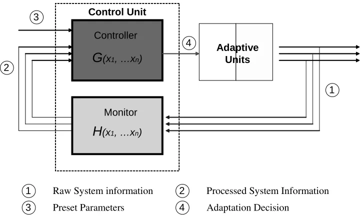
Figure 3.1: CiC feedback control model

adaptive targets on the chip. The resulting question is how to effectively manage these

adaptation possibilities to maximize the resource usage. We propose the CiC design model

to implement the system-wide analysis as an answer to this question.

The key point of CiC is guiding runtime optimizations with the consideration

of overall system performance and different optimization tradeoffs by using system-wide

information instead of local information. There are two fundamental functions related to

CiC design - distributed system information collecting and centralized information analysis.

Corresponding to these two functions, there are two logic components inside CiC - a monitor

and a controller. The monitor is in charge of collecting system-wide information and the

(33)

3.2 CiC logical feedback control model

The CiC logic model is shown in Figure 3.1. Logically, the CiC adaptation

proce-dure can be represented by a feedback control model. There are two main elements in this

control system: the adaptive unit(s) and the control unit. The adaptive unit is the target

of the adaptive design, typically it is one of the hardware components or parameters of a

processor. Unlike a fixed-parameter design, an adaptive unit features extra control circuitry

that enables reconfiguration during program execution. Typical examples of adaptive units

are as follows.

• caches and TLBs - line size or associativity is adjusted to accommodate distinct

memory access patterns.

• memory hierarchy - cache resources are divided among levels of the memory hierarchy.

• branch predictor - the length of global history register can be varied during execution.

• issue window - parts of the issue window is disabled for power efficiency when the

entire issue window is not needed.

• pipeline- a portion of the pipeline resources can be turned off to save power or pipeline

can switch between in order, out-of-order, and pipeline gating modes of operation.

The control unit is the core of the CiC model. It is in charge of making adaptation decisions.

As Figure 3.1 shows, it consists of a monitor and a controller. The monitor is on the path

of the feedback loop that transmits the runtime system information back to the controller.

(34)

input of the monitor is raw system information that is related to the adaptation schemes.

The output of the monitor is the processed system information, because the raw information

can not be used for adaptation decisions directly. Usually, information processing is based

on a specific analytical model. The input of the controller consists of two parts - one is the

processed system information from the output of the monitor. The other is some preset

built-in parameters, such as threshold values that come from empirical experiments. The

output of the controller is the adaptation decision that changes the configuration of the

adaptive unit at runtime.

The CiC operation cycle is as follows.

• The monitor collects related system information across the chip. Typically, data is

collected at a fixed sampling period.

• The monitor processes the collected information, feeds the processed information back

into the controller.

• The controller analyzes the information feed and makes an adaptation decision based

on an adaptation algorithm.

• The adaptive unit tunes its configuration according to the controller’s decision.

• The reconfigured adaptive unit changes the related system information. And then a

new CiC operation cycle starts. The monitor will feed the changed system information

back into the control loop to show the effectiveness of the previous adaptation decision

(35)

L2 Cache Decoder Fetch Logic Issue Queue IL1 Sch e d u le r ROB

Int FU FP FU L/S U

Renaming ITLB DL1 DTLB A rc h T a b R e n T a b S h a d o w T a b B T B B ra c h P re d R A S In s t B u ffe r Int Queue FP Queue Load/Store Queue Reg File

Int Regs FP Regs

Decoder

Fetch Logic

Renaming Int Queue

FP Queue R e n T a b Decoder Fetch Logic Mo n ito r C o n tro lle r

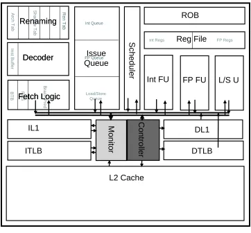
Figure 3.2: An example CiC floorplan

3.3 CiC chip floorplan

An example implementation of CiC chip floorplan is shown in Figure 3.2. It is a

hardware implementation of the CiC logic model. There is a dedicated onchip hardware

component - control unit that monitors and controls system optimizations. The monitor

implementation is similar to an event counter design, where an event detector resides in each

target component. When a corresponding event occurs, a signal is created to increment the

counter. For a sampling period, the event counters is read by the monitor and reset. And

(36)

vector and feed it into the controller. The controller is an application specific module to

(37)

Chapter 4

Methodology

4.1 Simulator

The simulator used in this study was derived from the SimpleScalar/Alpha 3.0 tool

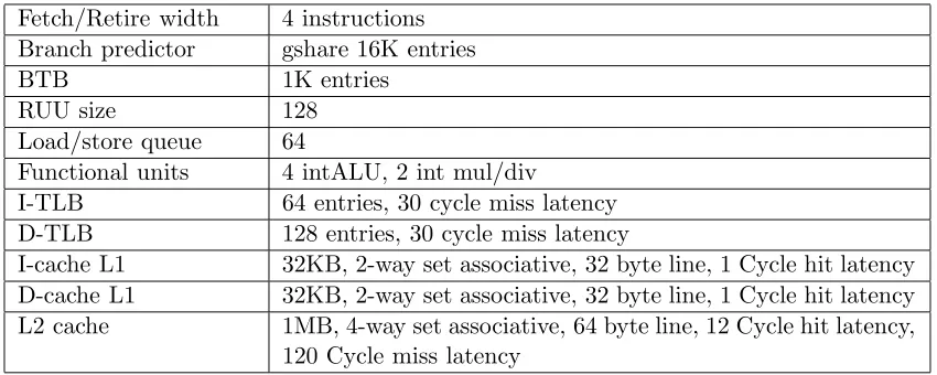
set [7], a suite of functional and timing simulation tools for the Alpha AXP ISA. Table 4.1

presents the configuration parameters for the baseline microarchitecture.

4.2 Benchmarks

This work studies 12 SPEC 2000 integer benchmarks. They aremcf, parser, vpr,

gzip, crafty,gcc,gap,parser,perl,eonandtwolf. Each program was simulated for 10

Billion committed instructions from the beginning. The benchmark details are presented

(38)

Table 4.1: Architectural configurations Fetch/Retire width 4 instructions

Branch predictor gshare 16K entries

BTB 1K entries

RUU size 128

Load/store queue 64

Functional units 4 intALU, 2 int mul/div

I-TLB 64 entries, 30 cycle miss latency D-TLB 128 entries, 30 cycle miss latency

I-cache L1 32KB, 2-way set associative, 32 byte line, 1 Cycle hit latency D-cache L1 32KB, 2-way set associative, 32 byte line, 1 Cycle hit latency L2 cache 1MB, 4-way set associative, 64 byte line, 12 Cycle hit latency,

120 Cycle miss latency

Table 4.2: The benchmarks studied in this dissertation benchmark input description

gzip input.source Compression

vpr *.in FPGA circuit placement and routing gcc 166.i C programming language compiler mcf inp.in Combinatorial optimization crafty crafty.in Chess game playing

parser ref.in Word processing eon chair Computer visualization perl splitmail PERL programming language gap ref.in Group theory, interpreter vortex lendian Object-Oriented database bzip2 input.source Compression

(39)

Chapter 5

Performance Bottleneck Modeling

The function of CiC monitor is collecting system-wide performance information for

performance bottleneck analysis. This chapter presents the performance bottleneck model

in detail.

5.1 Performance modeling

The performance of a modern microprocessor benefits from improvements in both

circuit technology and microarchitecture. Over the past decade, a typical

microarchitec-ture has evolved from in-order and scalar to out-of-order and superscalar with speculative

execution. However, as processors enjoy high instruction level parallelism from modern

mi-croarchitectures, system-level performance becomes harder to understand and the question,

“Where have the cycles gone ?”, becomes harder to answer, because many events overlap

and interact with each other. An effective performance analysis becomes more essential

(40)

optimizations.

There are many approaches developed to analyze program performance. The most

convenient way is software-based analysis tools, such as simulation [21, 5, 33] and

instru-mentation [51]. Simulation can provide details of program behavior, but causes several

orders of magnitude slowdown. Instrumenting original code can catch dynamic events, but

there still is code overhead and also the instrumentation code may change the behavior

of the original program. On the hardware side, modern microprocessors started providing

hardware support for performance analysis, called event counters [55, 50]. These counters

give an inside view of how the program interacts with the underlying hardware. Users can

access the counters with operating system and library support.

Modern microprocessors are able to execute a program at a speed of millions

of instructions per second. As a result, long-term program behavior interests researchers

because of the potential long-term optimizations, such as power and thermal management.

It has been shown that programs exhibit periods of similar behavior during their execution,

called program phases [3, 13, 45]. The reason of the phase phenomena is the regularity of

code execution. Tracking the footprint of instructions [45] and working sets [13] are typical

approaches to capture program phases.

Performance bottlenecks are both hardware and software dependent. Hardware

limitations, such as limited cache capacity, can slowdown program execution. The

charac-teristics of a program impacts performance as well, such as the amount of available inherent

code parallelism. Most previous performance bottleneck analysis are either profiling based

(41)

Next- PC logic BTB RAS PC +1 Ctl target MUX

I -TLB L1 Icache

L2 Cache MEM On-chip Off- chip L1 Dcache In st. B uff er IF Decoder Rename Table Arch map Shadow map ID IS Int Inst queue FP Inst queue Load Store queue

RR EX WB RE

A c ti v e Li s t F ree Li st Int Reg file FP Reg file

fu fu fu fu

Integer Exe Unit

fu fu

FP Exe Unit

Load & Store Unit

D -TLB BP

Figure 5.1: 7 stage out-of-order superscalar microarchitecture

instruction execution. In this paper, we analyze performance bottlenecks from a long-term

point of view. Unlike previous long-term work that catch the regular patterns of program

behavior to predict performance changes, our work provides a system-wide performance

diagnosis to find out what causes the current performance change and what the next

per-formance bottleneck will be.

In our work, we propose

• A counter-based long-term performance model to quantify the performance impact of

different system events,

• A bottleneck vector based bottleneck phase tracking scheme to capture program

bot-tleneck behavior at runtime,

(42)

5.2 Performance bottlenecks

Performance becomes hard to understand in a modern superscalar out-of-order

microprocessor because of the increasing number of inflight instructions and the

interac-tions between them. Therefore, it is necessary to review the instruction flow of a modern

microarchitecture and the potential factors that could cause performance slowdowns, before

we do further performance bottleneck analysis.

5.2.1 Superscalar out-of-order microarchitecture

Figure 5.1 shows a 7-stage out-of-order microarchitecture. The stages are IF

(In-struction Fetch), ID (In(In-struction Dispatch), IS (Issue), RR (Register Read), EX

(Execu-tion), WB (Writeback) and RE (Retire).

In the IF stage, the next instruction logic produces the next PC the processor

will fetch. The BTB (Branch Target Buffer) identifies the type of the current instruction.

For conditional branches, the branch predictor is involved for making a Taken/NotTaken

prediction. Unconditional branches are always predicted taken and the next PC is obtained

from this BTB entry. Return instructions are a special case where a RAS (Return Address

Stack) provides the return address. Otherwise, the default next PC is current PC plus one.

After generating (predicting) the next instruction address, the fetch engine accesses the

memory hierarchy to fetch the instructions into the pipeline.

In the ID stage, the fetched instruction is decoded first. Registers are renamed.

The source register is renamed by checking the renaming table. The output register gets a

(43)

is updated. Then, this renamed instruction is dispatched into the instruction issue queue

to wait for issuing.

In the IS stage, ready instructions are selected to move to EX stage, if the

corre-sponding functional units are available and issue logic has enough bandwidth.

In the RR stage, the issued instructions read values from the integer or floating

point register files or the forwarding paths.

In the EX stage, the ALU or the Floating-Point Unit executes instructions. The

execution latency is dependent on the type of instruction. Typically, division is the most

expensive instruction. Load instructions have variable latencies that depend on whether

they hit or miss in the L1 or the L2 cache.

In the WB stage, the outcome of EX stage is written back to the register file. Also,

the mispredicted branches are recovered in this stage.

In the RE stage, the instruction retires if it is safe. If the exception bit is set

for this instruction, recovery operations take place. All instructions after the exceptional

instruction are flushed and refetched.

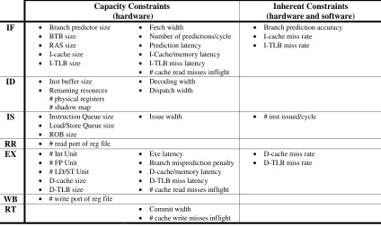
5.2.2 Potential performance bottlenecks

There are many factors that can lead to performance loss. Based on whether the

performance constraints are hardware or software dependent, we classify those constraints

into two categories - capacity constraints and inherent constraints, which are listed in Figure

5.2. The capacity constraints are caused by limited hardware resources, such as cache size,

or read/write ports. The inherent constraints are both hardware and software dependent.

(44)

Capacity Constraints (hardware)

Inherent Constraints (hardware and software) IF • Branch predictor size

• BTB size

• RAS size

• I-cache size

• I-TLB size

• Fetch width

• Number of predictions/cycle

• Prediction latency

• I-Cache/memory latency

• I-TLB miss latency

• # cache read misses

• Branch prediction accuracy

• I-cache miss rate

• I-TLB miss rate

ID • Inst buffer size

• Renaming resources # physical registers # shadow map

• Decoding width

• Dispatch width

IS • Instruction Queue size

• Load/Store Queue size

• ROB size

• Issue width • # inst issued/cycle

RR • # read port of reg file EX • # Int Unit

• # FP Unit

• # LD/ST Unit

• D-cache size

• D-TLB size

• Exe latency

• Branch misprediction penalty

• D-cache/memory latency

• D-TLB miss latency

• # cache read misses inflight

• D-cache miss rate

• D-TLB miss rate

WB

RT • Commit width

• # cache write misses inflight inflight

• # write port of reg file

(45)

well as the branch characteristics of the program.

5.3 Counter-based performance bottleneck modeling

In this section, we present an event counter based performance model. For modern

microprocessors, event counters are becoming a standard on-chip resource. Utilizing event

counters is a low overhead mechanism to monitor the behavior of microprocessor execution.

However, for modern complex microarchitectures, event counters are not accurate enough

for fine-grain instruction-level performance analysis because of the overlapping of events and

the interaction between instructions. But, from a long-term program performance point of

view, the overlapping effect can be approximately modeled with the event counter statistics.

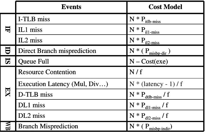
The goal of our counter-based performance model is to provide runtime

perfor-mance information to identify the perforperfor-mance bottlenecks that a microprocessor suffers.

As we described in Section 5.2.2, there are many constraints that impact performance.

With the consideration of hardware cost/effectiveness, investing the limited event counters

to those critical events is a reasonable choice. For our generic superscalar

microarchitec-ture, the critical events we choose are: I-TLB miss, IL1 miss, IL2 miss, direct unconditional

branch mispredictions, issue queue being full, resource contention, expensive instructions,

D-TLB miss, DL1 miss, DL2 miss and rest of branch mispredictions. While other events

may be critical for a specific architecture or execution situation, these critical events we

define are enough to reveal the general performance behavior. In addition, our analysis

(46)

N * (latency - 1) / f

Execution Latency (Mul, Div…)

N * P

_dl1-miss

/ f

DL1 miss

N * P

_dl2-miss

/ f

DL2 miss

N * ( P

_misbp-indir

)

Branch Misprediction

N * P

_dtlb-miss

/ f

D-TLB miss

N / f

Resource Contention

E

X

N – Cost(exe)

Queue Full

IS

Direct Branch misprediction

N * ( P

misbp-dir

)

ID

IL2 miss

N * P

il2-miss

N * P

_il1-miss

IL1 miss

N * P

_itlb-miss

I-TLB miss

IF

Cost Model

Events

Execution Latency (Mul, Div…)

N * P

_dl1-miss

/ f

DL1 miss

N * P

_dl2-miss

/ f

DL2 miss

N * ( P

_misbp-indir

)

Branch Misprediction

N * P

_dtlb-miss

/ f

D-TLB miss

N / f

Resource Contention

E

N – Cost(exe)

Queue Full

IS

Direct Branch misprediction

N * ( P

misbp-dir

)

ID

IL2 miss

N * P

il2-miss

N * P

_il1-miss

IL1 miss

N * P

_itlb-miss

I-TLB miss

IF

Cost Model

Events

WB

Figure 5.3: Performance model

5.3.1 Long-term event cost model

The counters give the numbers of critical events for a sampling interval. However,

these numbers can not tell us how important each of them is from the whole

microproces-sor performance viewpoint. For example, we should treat L1 cache misses and L2 cache

misses differently, because the miss latency difference between them is almost 10 fold. It

is clear that different critical events have a different impact on the overall microprocessor

performance. Our model tries to translate those raw numbers of different events into a

quantitative representation of performance. The modeling of each event is shown in Figure

5.3.

• I-TLB miss: An I-TLB miss causes a fetch engine stall. The cost of I-TLB miss

(47)

when instruction fetch is stalled, a pipeline bubble will be created during the waiting

period.

• I-L1 miss: The cost of I-L1 misses is the product of the number of events and the I-L1

miss penalty.

• I-L2 miss: The cost of I-L2 misses is the product of the number of events and the I-L2

miss penalty.

• Direct branch mispredictions: An unconditional direct branch misprediction causes a

pipeline flush. The cost of direct branch mispredictions is the product of the number

of events and branch misprediction penalty. The reason is the ID stage is still in

in-order and a pipeline bubble will be created during the period of waiting for pipeline

recovery.

• Resource Contention: Some instruction types will be stalled if there are not enough

idle functional units. The cost of resource contention is the event number divided by

a parallelism coefficientf, because resource contention doesn’t cause a whole pipeline

stall. Other type ready instructions can execute without waiting. So the performance

impact of resource contention is proportional to the number of contention events and

inversely proportional to the ILP. Since IPC is an approximation of available ILP, the

coefficient fwe choose is IPC plus one. The addition is to avoid amplifying the event

cost when IPC is less than 1.

• Expensive Instructions: Some expensive instructions, such as division, take a longer

(48)

events and the extra execution latency divided by the parallelism coefficient f.

• D-TLB miss event: The cost of D-TLB misses is the product of the number of events

and D-TLB miss penalty divided by parallelism coefficient f.

• D-L1 miss event: The cost of D-L1 misses is the product of the number of events and

D-L1 miss penalty divided by parallelism coefficient f.

• D-L2 miss event: The cost of D-L2 misses is the product of the number of events and

D-L2 miss penalty divided by parallelism coefficient f.

• Rest of branch mispredictions: Mispredicted conditional branches and indirect branches

cause a longer instruction fetch engine stall. The cost is the product of the number

of events and the misprediction penalty.

• Issue queue being full: The issue queue being full causes a pipeline stall. But the stall

in EX stage is the major reason of issue queue being full. So the cost of issue queue

being full is the number of events minus the cost of events in EX stage.

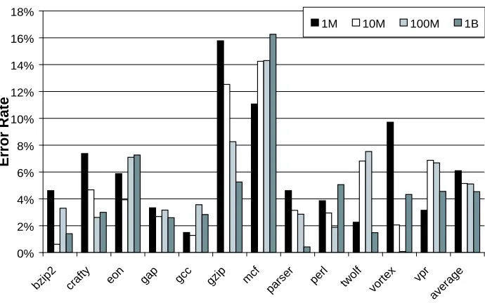
5.3.2 Model verification

The goal of our cost model is to quantify the performance effects of events based

on the bubbles that are inserted into the pipeline. The straightforward way to verify our

cost model is to compare the actual execution cycles to the sum of the execution cycles in

an ideal pipeline (i.e. pipeline throughput without bubbles) and the event costs from our

(49)

Tmodel =Tideal+ X

i

Costi (5.1)

Rerror =|Treal−Tmodel|/Treal (5.2)

In Formula 5.1, the predicted execution time (Tmodel) from our model is computed

by adding the ideal execution time (Tideal) and the total event cost (Costi). The ideal

execution time is the number of executed instructions divided by the issue width, assuming

each pipeline stage takes one cycle. Formula 5.2 represents the relative model error rate

(Rerror) calculated by dividing the absolute value of the difference between real execution

time and predicted execution time with the real execution time. Figure 5.4 shows the error

rate for different execution periods - 1M, 10M, 100M and 1B instructions. On average, our

model can achieve a 5% error rate, when l0M or more instructions are executed.

5.4 Performance bottleneck phase tracking

In the previous section, we presented an approach to collect system performance

information. Now we discuss how to analyze performance bottlenecks based on that

infor-mation.

5.4.1 Bottleneck vector

Choosing an appropriate quantitative representation is very important for data

analysis. A good representation can make analysis much easier and more accurate. For our

(50)

0% 2% 4% 6% 8% 10% 12% 14% 16% 18%

bzip2 crafty eon gap gc c

gzip mcf par

ser per l

two lf

vortex vp r

aver age

E

rror

R

a

te

1M 10M 100M 1B

Figure 5.4: Performance model verification

reasons why we use a vector. The first is that the data we collect are disjoint values in event

counters. These counters convey different information about different components in the

microprocessor and will be handled separately. Therefore, keeping data in a vector will be

a proper way without information loss. The other reason is that vectors are a powerful and

fundamental mathematical representation. Computations based on vectors are relatively

easy in both computation and hardware cost.

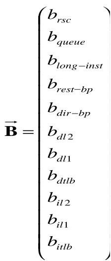
Based on the event counters we described in the last section, the bottleneck vector

has eleven dimensions which corresponds to each counter. The vector design is shown in

(51)

5.4.2 Bottleneck phases

Researchers proposed the program phase concept to describe the phenomena that

a program exhibits repeating long-term behavior. The principle behind program phases is

executing instructions visiting the static program with regular patterns. For example, in a

loop, the static loop body will be visited repeatedly during execution. It is not a surprise

that program phase phenomena has a similar effect on performance bottlenecks because

performance bottlenecks are determined by both hardware and software. With a fixed

hardware configuration, regular software patterns result in regular bottleneck behavior,

called bottleneck phases.

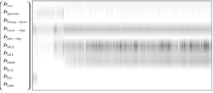
To illustrate the bottleneck phase behavior, we track the bottleneck vectors for

12 SPEC 2000 benchmarks for a 10B instruction execution, which is sampled every 1M

instructions. Each element of the vector is shown in parallel in the behavior graph. The

bottleneck intensity is represented by darkness. The darker the points are, the more intense

the performance bottleneck is. Figure 5.6, 5.7, 5.8, 5.9 and 5.10 show each benchmark

performance bottleneck behavior respectively.

• bzip2

Bzip2 varies its behavior during execution. It suffers from issue queue being full,

branch mispredictions and data cache misses intermittently.

• gap

Gap exhibits very regular behavior. There are very few outstanding performance

bottleneck during execution. Only in a very short period, it suffers from issue queue

(52)













=

− − − itlb il il dtlb dl dl bp dir bp rest inst long queue rsc

b

1 2 1 2

B

Figure 5.5: Bottleneck Vector

• gcc

Gcc varies its behavior over the whole execution time. It suffers from issue queue being

full, instruction cache misses, data instruction cache misses and branch misprediction

for different periods.

• mcf

Mcf suffers extremely from a high data cache miss bottleneck. But in the beginning,

it is bottleneck-free.

• vpr

Vpr suffers from data cache misses and branch misprediction bottlenecks at same

(53)

                                      − − − itlb il il dtlb dl dl bp dir bp rest inst long queue rsc b b b b b b b b b b b 1 2 1 2

Figure 5.6: bzip2 performance bottleneck behavior

Figure 5.7: gap performance bottleneck behavior

(54)

Figure 5.9: mcf performance bottleneck behavior

(55)

5.4.3 Bottleneck phase tracking

Identifying bottlenecks is not a difficult task from a mathematical perspective. We

can use the vector itself as an ID. However, hardware cost and computation complexity will

make this design very expensive. One efficient way to keep component cost information

without involving too much hardware budget is hashing the elements of the bottleneck vector

into a phase ID. The tracking scheme is shown in Figure 5.11. For a given sampling interval,

event counters are sampled and cleared. Then those raw event numbers are processed by

an array of function blocks. The function blocks perform two computations. One is average

cost computation based on the cost model. In our study, we use cost per 1K instructions

as the average cost for a sampling interval. The other is cost normalization computation,

which is translating the cost from the first step into the number of cost units. The cost

unit is a fixed cost window defined by users, depending on the accuracy requirement. The

reason for using the cost unit is to classify similar cost values into the same cost group.

Finally, the elements of the processed bottleneck vector are hashed into a bottleneck phase

ID.

5.5 Performance bottleneck phase prediction

In the previous section, we described how to track and identify a bottleneck phase

at runtime. There may be a need to predict bottlenecks in advance to guide system

opti-mization. In this section we will present the predictability of performance bottlenecks with

several prediction schemes.

Controller in Core: An Adaptive Microarchitectural Model for System-level Optimization

Contents

List of Figures

List of Tables

Chapter 1

Introduction

Chapter 2

Related Work

2.1

Energy-efficient adaptive microarchitectures

2.2

Temperature-aware microarchitecture

2.3

Performance-oriented adaptive microarchitectures

2.4

Performance modeling

2.5

Long-term program behavior

2.6

Value prediction

Chapter 3

Controller in Core

3.1

CiC concept

G

H(x

3.2

CiC logical feedback control model

3.3

CiC chip floorplan

Chapter 4

Methodology

4.1

Simulator

4.2

Benchmarks

Chapter 5

Performance Bottleneck Modeling

5.1

Performance modeling

5.2

Performance bottlenecks

5.3

Counter-based performance bottleneck modeling

N * (latency - 1) / f

Execution Latency (Mul, Div…)

N * P

/ f

DL1 miss

N * P

/ f

DL2 miss

N * ( P

)

Branch Misprediction

N * P

/ f

D-TLB miss

N / f

Resource Contention

E

X

N – Cost(exe)

Queue Full

IS

Direct Branch misprediction

N * ( P

)

ID

IL2 miss

N * P

N * P

IL1 miss

N * P

I-TLB miss

IF

Cost Model

Events

Execution Latency (Mul, Div…)

N * P