Impervious Surface Estimation Using Remote
Sensing Images and GIS: How Accurate is The
Estimate at Subdivision Level?
M. Rafee Majid
Department of Urban and Regional Planning, Faculty of Built Environment, Universiti Teknologi Malaysia, 81310 Skudai, Johor. Email:[email protected]
ABSTRACT: Impervious surface has long been accepted as a key environmental
indicator linking development to its impacts on water. Many have suggested that there is a direct correlation between degree of imperviousness and both quantity and quality of water. Quantifying the amount of impervious surface, however, remains difficult and tedious especially in urban areas. Lately more efforts have been focused on the application of remote sensing and GIS technologies in assessing the amount of impervious surface and many have reported promising results at various pixel levels. This paper discusses an attempt at estimating the amount of impervious surface at subdivision level using remote sensing images and GIS techniques. Using Landsat ETM+ images and GIS techniques, a regression tree model is first developed for estimating pixel imperviousness. GIS zonal functions are then used to estimate the amount of impervious surface for a sample of subdivisions. The accuracy of the model is evaluated by comparing the model-predicted imperviousness to digitized imperviousness at the subdivision level. The paper then concludes with a discussion on the convenience and accuracy of using the method to estimate imperviousness for large areas.
Keywords: impervious surface, imperviousness, regression tree method, remote
sensing images, GIS
Introduction
accuracy after aggregation at the subdivision level. Thus, this paper will investigate the potential of using Landsat ETM+ images for fast estimation of subdivision imperviousness by comparing the accuracy of the estimated imperviousness to that obtained through visual interpretation of 0.3m orthophotos. Due to its relatively high accuracy, imperviousness estimated through visual interpretation of a high-resolution aerial photo can be considered as the actual value of imperviousness in the field (Lee, 1987; Harvey, 1985; Kienegger, 1992).
Impervious surface is not a single homogeneous quantity but when used as a landscape indicator it is typically presented as a percentage of the land that is covered with impervious materials. Arnold & Gibbons (1996) defined impervious surfaces as any material covering the ground that prevents infiltration of water into the soil. While the prevalent man-made materials such as paved surfaces (roads, parking lots, sidewalks, etc.) and building rooftops fall unambiguously under the definition of impervious surfaces, there are other surfaces, man-made and natural, that are so heavily compacted as to be functionally impervious. Examples of these are compacted soil in construction areas, dirt roads, bedrock outcrops and, even to a certain extent, grass turf in residential areas (Arnold & Gibbons, 1996; Schueler, 1995). In this study, impervious surface was defined as any fixed man-made materials in a residential subdivision that has the potential to prevent infiltration of water into the soil. The materials may be used for functions that are related to dwelling such as rooftops and patios or transportation such as roads, parking and sidewalks or recreation such tennis court and swimming pool or infrastructures such as water tank, etc. Imperviousness, meanwhile, was defined as the extent of coverage by impervious surfaces in an area, regularly reported in percentage of the total area. As an environmental indicator, imperviousness has the advantage of being able to be measured at all scales of development.
Remote Sensing and Impervious Surface
.
(Brabec et al., 2002). Imperviousness in the early research was evaluated in four ways: 1) identifying impervious areas on aerial photography and then measuring them using a planimeter (e.g. Stafford et al., 1974; Graham et al., 1974); 2) overlaying a grid on an aerial photograph and counting the number of intersections that overlaid a variety of land uses or impervious features (e.g. Gluck & McCuen, 1975; Hammer, 1972; Ragan & Jackson, 1975); 3) supervised classification of remotely sensed images (e.g. Ragan and Jackson, 1975); and 4) equating the percentage of urbanization with the percentage of imperviousness (e.g. Morisawa & LaFlure, 1979). A number of studies also showed a significant correlation between total imperviousness and a number of demographic variables such as population density, number of households, employment, etc. (see Stankowski, 1972, Graham et al., 1974, Gluck & McCuen, 1975) but the relationship was site specific and some of the variables were not appropriate for all urban areas.
Early impervious surface mapping efforts using remotely sensed data were mainly conducted through visual interpretation of aerial photography. Manual identification of landscape features by aerial photograph interpretation and classification is time consuming and prohibitively expensive when performed over a large area. In addition, available aerial photographs are collected at differing scales and on different dates, thus requiring time-consuming rectification, digitization, and interpretation. With the launch of the Landsat Multispectral Sensor in 1972, digital satellite imagery began providing a synoptic view of the Earth’s surface capable of producing regular, repeatable land cover maps. Significant reductions in the amount of labor necessary for impervious surface delineation came with computer-automated spectral analysis of satellite data. These methods were capable of obtaining results comparable to aerial photo interpretation in considerably less time and with a significant reduction in cost (Ragan & Jackson, 1975).
aerial photographs is that satellite sensors have spectral bands that match the spectral reflectance properties of certain land covers. The Landsat TM (Thematic Mapper) sensor, for example, has six reflective bands whereas color and color-infrared aerial photography is limited to three spectral bands, and black and white photographs have only one band. There are, however, some limitations to satellite imagery. One major limitation is the relatively large pixel size (unit of resolution) of the images. Landsat TM images, for instance, have a pixel size of 30m x 30m, which is large enough such that individual pixels in urban areas typically encompass a diversity of land-cover conditions of differing imperviousness. In contrast, aerial photographs generally have much finer resolution (inches to a few feet), enabling the image analyst to distinguish one land cover from another. There are, however, satellite imagery with finer resolution such as IKONOS imagery (4m x 4m for multispectral image, 1m x 1m for panchromatic image) but the costs are rather prohibitive for a large study area that requires multiple scenes.
Many of the earlier methods using spectral information from satellite sensors are based on supervised and unsupervised classification techniques and other forms of spectral clustering, thresholding, and modeling. Products are often presented as maps portraying the presence or absence of impervious features at the single pixel scale. Other estimates of impervious cover, meanwhile, rely on lookup tables (conversion factors) derived from surrogate measures of parcel size (Monday et al., 1994; Sleavin et al., 2000) and land use and land cover information (Deguchi & Sugio, 1994; Williams & Norton, 2000; Ward et al., 2000). Forster (1985), however, warned against classifying MSS and TM pixels found in the urban settings as one specific land cover class due to a mismatch in resolutions; the sensor resolution being too coarse compared to the fine spatial resolution of features in the urban environment.
.
municipalities in Connecticut, USA using artificial neural network and an ERDAS Imagine® subpixel classifier. The overall accuracy at the binary impervious-non-impervious detection level varied from 71 to 94% with a root mean square error (RMSE) of 0.66 to 5.97. Spectral mixture modeling is another method that can be used to estimate subpixel land cover information. Ji and Jenson (1999), Wu and Murray (2002), Ward et al. (2000), and Rashed et al. (2003) have used this method to derive information about the amount of impervious cover in a single pixel. Wu and Murray reported an overall estimation RMSE of 10.6 percent imperviousness.
In another approach, modeling techniques using decision tree models have been successfully implemented in subpixel quantification of impervious surface. A decision tree model dealing with discrete data is known as a classification tree model and that dealing with continuous data is referred to as a regression tree model. Smith (2000), for instance, used classification tree for Montgomery County, Maryland, USA with the overall within-class accuracy of about 84%. Yang et al. (2003) went a step further by using regression tree, thus modeling the impervious surface output as a continuous rather than discrete variable. In order to check the applicability of their model at different spatial scales, Yang et al. conducted their study on three different spatial scales, i.e. a local scale of ~1000 km2, a subregional scale of ~10000 km2), and a regional scale of 100000 km2. Regardless of change in spatial scale, it was found that the technique was capable of predicting imperviousness with consistent and acceptable accuracy. For all three areas tested, the correlation coefficient between the predicted and actual imperviousness ranged from 0.82 to 0.91, and the average error varied from 8.8 to 11.4 percent imperviousness.
Study Area
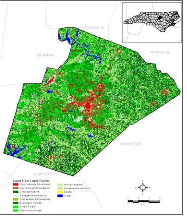
Figure 1: Study area showing land use disribution
For the purpose of this study, Wake County in the State of North Carolina, USA was selected as the study area (Figure 1). The area was selected because of data availability and logistical convenience for the author at the time of the study. With a land mass of 860 square miles, the county housed an estimated population of 627,846 in 2000 which was projected to be 678,651 persons in 2002 (U.S. Census Bureau, 2000). Wake County measures about 46 miles from east to west and 39 miles north to south. Based on the
.
Table 1: Distribution of land use in Wake County
Land Use/Land Cover Area (acres) Area (%)
High Intensity Developed Low Intensity Developed Crop agriculture Managed Herbaceous Unmanaged Herbaceous Evergreen Forest Mixed Forest Deciduous Forest Woody wetland Herbaceous Wetland Sands Water 21,903 17,941 73,097 29,437 65 212,340 90,470 2,955 84,332 16 861 15,814 4.0% 3.3% 13.3% 5.4% 0.01% 38.7% 16.5% 0.5% 15.4% 0.003% 0.2% 2.9%
TOTAL 549,231 100.0%
Methods and Procedures
Data Acquisition
Estimation of imperviousness using remote sensing images was carried out using two forms of remote sensing imagery and a planimetric data of a small section of the study area. The first type of the remote sensing imagery was scenes from Path 15/Row 35 and Path 16/Row 35 of the Landsat ETM+ images captured by
Landsat 7 satellite. The images that were captured on 25 April 2002 had already been orthorectified and projected to UTM Zone 17 coordinate system with a NAD83 datum (Figure 2). Orthorectified images are images that have been corrected from distortion due to sensor tilt and terrain-induced distortion.
Figure 2: Landsat ETM+ images
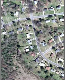
0.3m orthophotos of the study area are part of the Raleigh-Durham High Resolution Color Orthoimagery taken on 28 March 2002. The orthophotos have been orthorectified and projected to UTM Zone 17 coordinate system with a NAD83 datum (Figure 3). The high resolution of the orthophotos made it possible to visually compare between pervious and impervious materials as well as between different types of impervious materials. For that reason, the orthophotos were utilized to update the planimetric data used in establishing the training and validation data set for impervious surface. To avoid potential errors due to temporal difference in image dates, it is best that all the images are of the same date or at least close enough for assumption of no changes in land use/land cover properties. As it turned out, the acquisition dates of the orthophotos and the Landsat ETM+ images are close enough for the assumption, i.e. approximately one month difference.
Digital planimetric data for a small urbanized section of the county, i.e. the City of Raleigh, was acquired and utilized as the main source of training and validation data sets for impervious surface in building the regression tree model. The data were obtained from the City of Raleigh’s GIS Department and its coverage was limited to only the City of Raleigh. It is important to note here that although the planimetric data contained rich information in vector format delineating as-built boundaries of building footprints, parking lots, roads, footpaths and other structures, its use for determining the amount of impervious surface was limited by its
spatial availability. In this case, the planimetric data covers only about ten percents of the study area. On top of that, the currency of the planimetric data was lacking, requiring updating of information using the latest high-resolution aerial photos. With its information updated using the 0.3m orthophotos, the planimetric data provided an accurate and current training and validation data sets for impervious
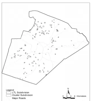
Direct estimation of imperviousness at subdivision level using aerial photos required usage of GIS spatial data in addition to the 0.3m orthophotos described above. The GIS data layers include: 1) a subdivision map for identification and random selection of subdivision samples, where a total of 115 samples out of the available 3280 subdivisions were selected (Figure 4); 2) planimetric data, used in conjunction with the orthophotos, to expedite digitizing of
impervious surface in subdivisions for which the planimetric data was available (i.e. within the City of Raleigh); and 3) a digital road network to expedite calculation of impervious surface originating from streets. All of the data used in this part are digital spatial data in ArcView shapefiles either downloaded from the Wake County GIS website or obtained directly from the municipalities in digital format via digital discs for the data not available
online. Figure 4: Locations of sampled subdivisions
Remote Sensing Image Pre-Processing
Before they could be used, the remote sensing images must go through a few steps of preprocessing. The original 28.5m ETM+ images were co-registered to the 0.3m orthophotos to within 0.5 pixel root mean squared error (RMSE) before being resampled to 30m pixels using the nearest neighbor resampling method. The 0.3m orthophotos themselves were beforehand co-registered to the planimetric data. Co-registration is a process of superposing two or more images guided by ground control points so that equivalent geographic points coincide. Accurate co-registration between the images is important since even a slight mis-registration could result in potentially large differences between actual and predicted values of imperviousness. All of these steps were done using the ERDAS Imagine 8.6 software.
Using the GIS software ArcView® 3.2 equipped with its spatial and image analysis extensions (Spatial Analyst and Image Analyst), the digital numbers (DN) of all six
reflective bands of the Landsat ETM+ images (Bands 1-5,7) were then converted to at-satellite reflectance values as described by Landsat Project Science Office (2002). Then the Normalized Difference Vegetation Index (NDVI) values for the images were calculated, followed by the Tasseled-cap values of brightness, greenness and wetness, using at-satellite reflectance-based coefficients described by Huang et al.
(2002). The ratio of Band 5:1 was also added as a possible soil moisture indicator helpful in discriminating between concrete and exposed soil. To summarize, the final layers that would be used as independent variable inputs were grid layers of at-satellite reflectance of ETM+ visible bands, NDVI values, Tasseled-cap values and Band 5:1 ratio (Table 2).
Table 2: Independent variables for regression tree method
Independent Variable Source Format
Band 1 Band 2 Band 3 Band 4 Band 5 Band 7 NDVI
Tasseled-cap Brightness Tasseled-cap Greenness Tasseled-cap Wetness Band 5: Band 1 Ratio
Landsat ETM+ Landsat ETM+ Landsat ETM+ Landsat ETM+ Landsat ETM+ Landsat ETM+
Landsat ETM+ (calculated) Landsat ETM+ (calculated) Landsat ETM+ (calculated) Landsat ETM+ (calculated) Landsat ETM+ (calculated)
30m raster grid 30m raster grid 30m raster grid 30m raster grid 30m raster grid 30m raster grid 30m raster grid 30m raster grid 30m raster grid 30m raster grid 30m raster grid
Training and Validation Data
.
utilities, etc) were merged into one vector dataset and reprojected from North Carolina State Plane Coordinates NAD83 into UTM Zone 17 coordinates in ArcView. Four 1800m x 1800m windows of the planimetric data were visually selected to cover spectral variations of impervious surfaces and degree of urbanization that best represent the study area. Each of the four 1800m x 1800m windows was then divided into nine equal-sized blocks of 600m x 600m where six of which were randomly selected for use as training blocks and the remaining three as validation blocks. Campbell (1981) and Friedl et al. (2000) suggested that using randomly selected pixel blocks rather than individual pixels as test data should reduce possible bias in model accuracy assessment due to spatial autocorrelation between training and test data. The updated planimetric data for training and validation were then rasterized into 0.3m pixel in ArcView and reclassified into binary categories of impervious and pervious. Zonal summary of the 0.3m pixels of the impervious category according to each 30m pixel of the training and validation areas were then carried out using the Spatial Analyst function of ArcView 3.2.
Regression Tree Analysis
Collection of the values for the independent and dependent variables was first carried out before starting the regression tree analysis. The task was carried out in ArcView with the help of an Avenue Extension called StatMod developed by Garrard of Utah State University (Garrard, 2002). StatMod was used to collect the grid values of both the independent and dependent variables from their respective grid layers. The independent variables were those listed in Table 2 and the dependent variable was the percentage of impervious surface within each 30m pixel of the four 1800m x 1800m training and validation areas explained in the previous section. A total of 9600 data points (grid values) per variable were collected for use as training data and 4800 data points per variable as validation data. The data were then exported from
to produce a series of simpler trees, each of which a candidate for the optimal tree. In order to select an optimal tree, the quality of each candidate tree was based on its mean absolute error of prediction (using the validation data). In addition to mean absolute error, correlation coefficient was also calculated for each candidate tree. Since several trees were close in their qualities, the tree that used the least number of independent variables, a parsimonious model, was selected. A parsimonious tree model was desirable since it required less data volume as well as computing time. For further reading on the regression tree method, readers are encouraged to refer to Breiman et al. (1984).
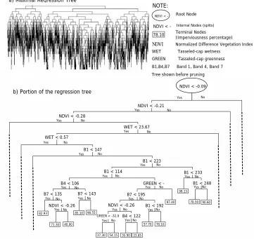
a) Maximal Regression Tree
NDVI < - Root Node
NDVI < - Internal Nodes (splits) 78.10 Terminal Nodes (Imperviousness percentage)
NDVI Normalized Difference VegetationIndex NOTE:
WET Tasseled-cap wetness
.
B1 < 114
B1 < 223 B1 < 147
WET < 0.57
WET < 23.67 NDVI < -0.28
NDVI < -0.21
B1 < 233
GREEN < -B4 < 106
NDVI < -0.26
B7 < 135 B7 < 143 B7 < 195
B1 < 248
GREEN < -32.9 B4 < 122 NDVI < -0.26 B1 < 192
23.85 35.90 54.15 37.30 98.55 85.10 40.90 71.30 90.60 82.93 78.50 98.13 97.40 78.10 57.70
NDVI < -0.09
Yes No Yes Yes Yes No No No No No No No No No No No Yes Yes Yes Yes Yes Yes Yes Yes No No No No No No No Yes Yes Yes Yes Yes Yes No
Yes Yes
b) Portion of the regression tree
GREEN Tasseled-cap greenness B1,B4,B7 Band 1, Band 4, Band 7 Tree shown before pruning
Figure 5: Maximal regression tree without the variables (a) and details of a portion of the tree generated using S-PLUS (b).
Digitizing Impervious Surface of Subdivisions
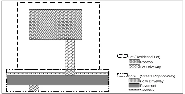
Transverse Mercator (UTM), North American Datum (NAD) 1983. From there, impervious surfaces as schematically shown in Figure 6 below were digitized from the orthophotos. The process entailed tracing each identifiable feature’s impervious footprint from the orthophotos and summing its total amount according to subdivision. Imperviousness value of each subdivision was then calculated which was the percentage of the total subdivision area covered with impervious surface.
Figure 6: Components of impervious surface in residential subdivisions Lot (Residential Lot)
r.o.w (Streets Right-of-Way) Rooftop
Lot Driveway
Pavement r.o.w Driveway
Sidewalk
of lot size within the subdivisions. The range of sample percentages was from five percent for subdivisions with homogeneous lots to as high as thirty percent for subdivisions with variable lot sizes.
Results and Discussions
Selecting the Optimal Model
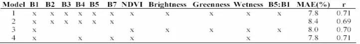
Table 3 lists accuracy estimates for some promising model options based on different combinations of independent variables. The mean absolute errors for the models range from 7.8 to 8.4% with the correlation coefficients range very closely from 0.69 to 0.71. These results are close to those reported by Yang et al. (2003) when they used the same model to estimate impervious surface. They reported mean absolute errors of 9.2 to 11.4% and slightly higher correlation coefficients of 0.82 to 0.89.
Table 3: Performance of selected models using different combinations of predictive variables
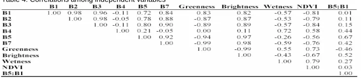
The small differences in accuracy estimates among the models encouraged adoption of a simpler and parsimonious model requiring the least number of independent variables. The relative importance of the independent variables was assessed based on the position of each variable within the rule-sets (the tree) of the model. Within the rule-sets, independent variables are ordered in decreasing relevance to the dependent variable with the most important independent variable positioned at the top of the tree. Figure 8b shows portion of the maximal regression tree generated in S-PLUS showing the relative importance of each independent variable in the tree. Inspection of the rule-setsof the models revealed that the most important variables in descending order were NDVI, wetness, B1, B7 and B4. The insignificance of the other variables excluded from the models was not surprising since there were high correlations among the variables as indicated in Table 4. The selected regression
tree model was therefore the one developed using only NDVI, wetness; B1, B4 and B7 (Model 4 in Table 3).
Table 4: Correlations among independent variables
Pixel-to-Pixel Accuracy
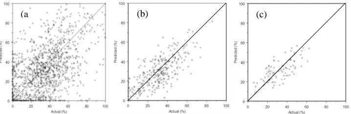
Validation of pixel imperviousness estimated by regression tree models using Landsat ETM+ images was poor on a pixel-by-pixel basis due to the geometric registration errors between the Landsat images and the orthophotos. Figure 7a shows the plot of predicted versus actual imperviousness on pixel-by-pixel basis. In general, image-to-image registration can rarely be less than half a pixel off in both horizontal and vertical directions. When comparing the subpixel impervious surface from these two sources on a pixel-by-pixel basis, there is less than a quarter of a pixel overlap. This small overlap is the reason why a small mismatch in the registration can lead to large errors in accuracy assessment (Dai and Khorram, 1998).
(c) (b) (a
Figure 7: Predicted versus actual imperviousness per pixel for a) 30m pixels, b) 60m pixels (2x2 windows) c) 90m pixels (3x3 window)
Accuracy through Visual Inspection Accuracy through Visual Inspection
Another way to assess the accuracy of the selected model is through visual inspection of predicted imperviousness over the entire study are. Application of the selected regression tree model over the entire study area produced reasonable spatial pattern of impervious surface with some weaknesses that could be overcome to a certain degree. The most obvious weakness was the confusion in interpreting water bodies as impervious surface but
this weakness was overcome in this study by implementing water mask to the study area. Water mask can be easily extracted from classification of the remote sensing images. The second and more difficult weakness was the spectral confusion between bare soils (especially from fallow fields) and man-made impervious surface that was believed to haveresulted in over prediction of low imperviousness as shown in Figure 8. This is however more a weakness of the remote sensing images than the model itself. In this study, this weakness was partly overcome by including a farm mask Another way to assess the accuracy
of the selected model is through visual inspection of predicted imperviousness over the entire study are. Application of the selected regression tree model over the entire study area produced reasonable spatial pattern of impervious surface with some weaknesses that could be overcome to a certain degree. The most obvious weakness was the confusion in interpreting water bodies as impervious surface but
this weakness was overcome in this study by implementing water mask to the study area. Water mask can be easily extracted from classification of the remote sensing images. The second and more difficult weakness was the spectral confusion between bare soils (especially from fallow fields) and man-made impervious surface that was believed to haveresulted in over prediction of low imperviousness as shown in Figure 8. This is however more a weakness of the remote sensing images than the model itself. In this study, this weakness was partly overcome by including a farm mask
Figure 8: Model-predicted imperviousness of the study area
extracted from the parcel map and assigning zero as the imperviousness value of the area. For urban area, however, there is no available data for such mask and it may or may not be reasonable to anticipate that the extent of bare soils in urban area is relatively minimal. This will be confirmed, at least in this study, when the comparison between predicted and actual imperviousness is done at subdivision level next.
Figure 8 shows the results of applying the final model over the entire study area with the water and farm masks discussed above incorporated. Visual inspection of the outputs indicates reasonable representation of the pattern of impervious surface within the study area. Major urban centers, the airport, shopping malls and even major transportation routes are well represented with very high imperviousness. High density residential areas within two major municipalities in the study area, Cary and Raleigh, are well differentiated from areas of low residential density surrounding them. These results are good enough for analysis at this level, i.e. a regional level.
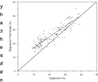
Accuracy at Subdivision Level
however still a tendency for the model to overpredict imperviousness at low values. This can be attributed to confusion in Landsat images between bare soils and impervious surface.
however still a tendency for the model to overpredict imperviousness at low values. This can be attributed to confusion in Landsat images between bare soils and impervious surface.
Conclusions Conclusions
The study was about application of remote sensing technology in urban planning works. The objective here was investigate the accuracy of using medium-resolution Landsat ETM+ images in estimating impervious surface aggregated at subdivision level. Images from Landsat ETM+ were
used together with GIS-ready planimetric data updated with high resolution orthophotos for developing a regression tree model to predict imperviousness percentage of each Landsat pixel. Zonal summary of the imperviousness percentage of relevant pixels would give percentage of impervious surface within any spatial zone such as subdivisions, city or even county. It was found that there were several limitations of the model, some of
which could be overcome as discussed earlier. However, certain weaknesses seemed to be inherent of the model or the procedures involved in developing the model. One such weakness was the difficulty in co-registering the images used in the model which affected the accuracy of pixel-to-pixel model validation. Nevertheless, this difficulty was overcome by validating the results on aggregated window basis and the resulting prediction error of about 8% was comparable to those reported in past studies. More useful from management perspective, however, was aggregation of the predicted imperviousness at subdivision level which resulted in higher accuracy when compared to the digitized values. The mean absolute error reported was about 5% but there was still a tendency for the model to over predict imperviousness at low values due to confusion with bare soils. Although the mean absolute error of 5% is The study was about application of remote sensing technology in urban planning works. The objective here was investigate the accuracy of using medium-resolution Landsat ETM+ images in estimating impervious surface aggregated at subdivision level. Images from Landsat ETM+ were
used together with GIS-ready planimetric data updated with high resolution orthophotos for developing a regression tree model to predict imperviousness percentage of each Landsat pixel. Zonal summary of the imperviousness percentage of relevant pixels would give percentage of impervious surface within any spatial zone such as subdivisions, city or even county. It was found that there were several limitations of the model, some of
which could be overcome as discussed earlier. However, certain weaknesses seemed to be inherent of the model or the procedures involved in developing the model. One such weakness was the difficulty in co-registering the images used in the model which affected the accuracy of pixel-to-pixel model validation. Nevertheless, this difficulty was overcome by validating the results on aggregated window basis and the resulting prediction error of about 8% was comparable to those reported in past studies. More useful from management perspective, however, was aggregation of the predicted imperviousness at subdivision level which resulted in higher accuracy when compared to the digitized values. The mean absolute error reported was about 5% but there was still a tendency for the model to over predict imperviousness at low values due to confusion with bare soils. Although the mean absolute error of 5% is
Figure 9: Model-predicted imperviousness versus digitized imperviousness at subdivision level
encouraging, the tendency to overestimate low imperviousness can generate biased results. Overall the model has a potential for a quick and synoptic estimate of imperviousness in large areas provided that the areas have no or little bare soil or a procedure is available to eliminate bare soil interference in the model’s prediction.
Finally, even though the setting of the study was somewhat different from what we have here in Malaysia, the author believes that the principles and the techniques behind the study are still relevant if the study were to be applied here. The convenience of using remote sensing images for impervious surface estimation would still be applicable and should therefore be taken advantage of. Cautions, however, should be exercised when matching the objectives of the study to the resolution of the remote sensing images used and the issue of spectral confusion between impervious surface and bare soils or other similar natural features still needs to be resolved/duly noted.
References
Arnold, C.L. and C. J. Gibbons. 1996. Impervious surface: The emergence of a key urban environmental indicator. Journal of the American Planning Association 62(2): 243-258.
Brabec, E., S. Schulte and P.L. Richards. 2002. Impervious surfaces and water quality: A review of current literature and its implications for watershed planning. Journal of Planning Literature 16(4):499-514.
Breiman, L., J. Friedman, R. Olshen and C. Stone. 1984. Classification and Regression Trees. Chapman and Hall, New York. 358pp.
Campbell, J. 1981. Spatial correlation effects upon accuracy of supervised classification of land cover. Photogrammetric Engineering & Remote Sensing 47(3):355-63.
Civco, D.L. and J.D. Hurd. 1997. Impervious surface sapping for the State of Connecticut. Proceedings of the 1997 ASPRS Annual Conference, Seattle, WA. (124-135)
Dai, X. and S. Khorram. 1998. The effects of image miss-registration on accuracy of remotely sensed change detection. IEEE Trans. Geo-science and Remote Sensing 36:1566–1577.
.
Flanagan M, and D.L. Civco. 2001. Sub pixel impervious surface mapping. Proceedings of the 2001 ASPRS Annual Convention, 23–27 Apr.2001, St. Louis, MO.
Forster, B.C., 1985. An examination of some problems and solutions in monitoring urban areas from satellite platforms. International Journal of Remote Sensing 6(1):139-151.
Friedl, M.A., C. Woodcock, S. Gopal, D. Muchoney, A.H. Strahler and C. Barker-Schaaf. 2000. A note on procedures used for accuracy assessment in land cover maps derived from AVHRR data. International Journal of Remote Sensing 21:1073– 1077.
Garrard, C. 2002. StatMod. Available online at
http://bioweb.usu.edu/gistools/statmod/. Accessed on 11/20/2004.
Gluck, W.R. and R.H. McCuen. 1975. Estimating land use characteristics for hydrologic models. Water Resources Research 11(1):177-79.
Graham, P.H., S.C. Lawrence and H.J. Mallon. 1974. Estimation of imperviousness and specific curb length for forecasting stormwater quality and quantity. Journal of the Water Pollution Control Federation 46(4):717-25.
Hammer, T.R. 1972. Stream enlargement due to urbanization. Water Resources Bulletin 8(6):1530-40.
Harvey, R. B.1985. The Use of orthophotography and GIS technology to conduct a storm drainage utility impervious surface analysis: A case study. Proceedings ASPRS/ACSM Annual Meeting, 10 - 15 Mar 1985. Washington DC. pp271-78.
Huang, C., B. Wylie, L. Yang, C. Homer and G. Zylstra. 2002. Derivation of a tasseled-cap transformation based on Landsat 7 at-satellite reflectance. International Journal of Remote Sensing 23(8):1741–1748.
Kienegger, E.H. 1992. Assessment of Wastewater Service Charge by integrating Aerial photography and GIS. Photogrammetric Engineering and Remote Sensing 58(11):1601-1606.
Lee, K.H. 1987. Determining impervious area for stormwater assessment. Proceedings ASPRS/ACSM Annual Convention, 29 Mar - 3 Apr 1987. Baltimore, MD. pp17-23.
Monday, H.M., J.S. Urban, D. Mulawa and C.A. Benkelman. 1994. City of Irvine utilizes high resolution multispectral imagery for NPDES compliance. Photogrammetric Engineering & Remote Sensing 60(4): 411-16.
Ragan, R.M. and T.J. Jackson. 1975. Use of satellite data in urban hydrologic models. Journal of the Hydraulics Division ASCE 101: 1469-75.
Rashed, T., J.R. Weeks, D. Roberts, J. Rogan, and R. Powell. 2003. Measuring the physical composition of urban morphology using multiple endmember spectral mixture models. Photogrammetric Engineering & Remote Sensing 69(9):1011-20.
Schueler, T.R. 1995. The peculiarities of perviousness. Watershed Protection Techniques 2(1):233-39.
Slonecker, E.T., D.B. Jennings and D. Garofalo. 2001. Remote sensing of impervious surfaces: A review. Remote Sensing Reviews 20:227-255.
Smith, A.J. 2000. Subpixel estimates of impervious surface cover using Landsat TM imagery. M.A. Scholarly paper. Unpublished. Department of Geography, University of Maryland. College Park, MD.
Stafford, D.B., J.T. Ligon and M.E. Nettles. 1974. Use of aerial photographs to measure land use changes in remote sensing and water resources management. Proceedings 17, American Water Resources Association. American Water Resources Association. Herndon, VA.
Stankowski, S.J. 1972. Population density as an indirect indicator of urban and suburban land-surface modifications. U.S. Geological Survey Professional Paper 800-B. U.S. Geological Survey. Washington, DC.
U.S. Census Bureau. 2000. State and County Quickfacts. Available online at http://quickfacts.census.gov/. Accessed on 03/01/2003.
Ward, D., S.R. Phinn and A.T. Murray. 2000. Monitoring growth in rapidly urbanized areas using remotely sensed data. Professional Geographer 52(3):371–86.
Williams, D.J., and SB. Norton. 2000. Determining impervious surfaces in satellite imagery using digital orthophotography. Proceedings of the 2000 ASPRS Annual Conference. 22–26 May 2000. Washington, DC.
Wu, C. and A.T. Murray. 2002. Estimating impervious surface distribution by spectral mixture analysis. Remote Sensing of Environment 84:493-505.