R E S E A R C H
Open Access
Solving Robin problems in multiply
connected regions via an integral equation
with the generalized Neumann kernel
Shwan HH Al-Shatri
1, Ali HM Murid
1,2*, Munira Ismail
1and Mukhiddin I Muminov
1*Correspondence:
1Department of Mathematical
Sciences, Faculty of Science, Universiti Teknologi Malaysia, Johor Bahru, Johor, 81310, Malaysia
2UTM Centre for Industrial and
Applied Mathematics (UTM-CIAM), Ibnu Sina Institute for Scientific and Industrial Research, University Teknologi Malaysia, Johor Bahru, Johor, 81310, Malaysia
Abstract
This paper presents a boundary integral equation method for finding the solution of Robin problems in bounded and unbounded multiply connected regions. The Robin problems are formulated as Riemann-Hilbert problems which lead to systems of integral equations and the related differential equations are also constructed that give rise to unique solutions, which are shown. Numerical results on several test regions are presented to illustrate that the approximate solution when using this method for the Robin problems when the boundaries are sufficiently smooth are accurate.
Keywords: Robin problem; Riemann-Hilbert problem; integral equation; generalized Neumann kernel; multiply connected region
1 Introduction
A boundary value problem is a problem that involves finding the solution of a differential equation or system of differential equation which meets certain specified requirements or boundary conditions at the end points or along a boundary, usually connected with the physical condition for certain values of the independent variable. This paper considers
Laplace’s equationu= in both bounded and unbounded multiply connected regions
with a linear combination of Dirichlet and Neumann boundary conditions on the
bound-ary=∂, generally known as a mixed boundary value problem and commonly called
the Robin problem.
Applications of mixed boundary value problems exist in large numbers in classical math-ematical physics, physical geodesy, electro-magnetics, analysis of measurement [, ], and specific boundary problems such as the Dirichlet problem and the Neumann problem []. The applications of the mixed boundary value problem in potential theory can be found in [].
It has been shown that the problem of conformal mapping, the Dirichlet problem, the Neumann problem, and the mixed Dirichlet-Neumann problem can all be treated as Rie-mann Hilbert (briefly RH) problems as discussed in [–]. The interplay of RH problems and the boundary Fredholm integral equation with the generalized Neumann kernel has been investigated in [] for simply connected regions with smooth and piecewise smooth boundaries and in [] for bounded and unbounded multiply connected regions.
Earlier, the well-known integral equations for RH problem have been employed for solving the Dirichlet problem and the Neumann problem [] and the mixed Dirichlet-Neumann problem []. They are uniquely solvable Fredholm integral equations of the sec-ond kind. However, the problems in [] and [] are not Robin problems, since the Dirichlet condition and Neumann condition are given separately.
This paper solves the Robin problem by reducing it to a RH problem and hence providing a related system of boundary integral equations. Additional conditions are given to obtain a unique solution to the Robin problem.
This paper is organized as follows: After the presentation of some notations and auxil-iary material in Section , we present in Section , the reduction of the Robin problems in bounded and unbounded multiply connected regions to the RH problem. We then show how to construct the integral equations and differential equations related to the Robin problems. Conditions for obtaining unique solution for the Robin problems are also given. In Section , we show how to treat the integral equations and differential equations numer-ically. In Section , we give some numerical examples for several test regions. In Section we give a short conclusion.
2 Notations and auxiliary material
Consider a multiply connected regionin the extended complex planeCof the following two types []:
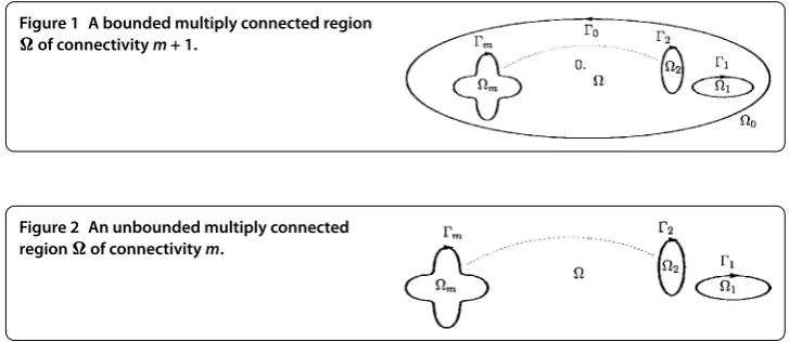
(a) A bounded regionof connectivitym+ ≥ with boundary=mj=jconsisting
ofm+ smooth closed Jordan curvesj,j= , , . . . ,m. The curvecontains the other curves, . . . ,m. The complement–:=C\consists ofmbounded simply connected
componentsjinterior toj,j= , , . . . ,m, and an unbounded simply connected
compo-nentexterior to(see Figure ). We assume that ∈.
(b) An unbounded regionof connectivitym≥ with boundary=mj=jconsisting
ofmsmooth closed Jordan curvesj,j= , , . . . ,m. The complement–:=C\consists
ofmbounded simply connected componentsjinterior toj,j= , , . . . ,m(see Figure ).
We assume that /∈.
The orientation of the boundary=∂is such thatis always on the left of. Thus, the curves, . . . ,m always have clockwise orientations. For bounded, the curve has a counterclockwise orientation. The curvesjare parameterized by π-periodic twice
Figure 1 A bounded multiply connected region
of connectivitym+ 1.
continuously differentiable complex functionsηj(t) with non-vanishing first derivatives,
˙
ηj(t) = dηj(t)
dt = , t∈Jj:= [, π],
j= (for bounded), , , . . . ,m. We represent the disjoint union of the intervalsJjbyJas a total parameter domain. Automatically, the whole boundarywill be parameterized by a complex functionηdefined onJby
η(t) :=
⎧ ⎪ ⎪ ⎪ ⎪ ⎨ ⎪ ⎪ ⎪ ⎪ ⎩
η(t), t∈J(for bounded),
η(t), t∈J, ..
.
ηm(t), t∈Jm.
Assume thatHbe the space of all real Hölder continuous functions on the boundary. Sinceηis smooth, a functionφ∈Hcan be interpreted viaφˆ(t) :=φ(η(t)),t∈J, as a real Hölder continuous π-periodic functionsφˆ(t) of the parametert∈J,i.e.,
ˆ
φ(t) :=
⎧ ⎪ ⎪ ⎪ ⎪ ⎨ ⎪ ⎪ ⎪ ⎪ ⎩
ˆ
φ(t), t∈J(for bounded),
ˆ
φ(t), t∈J, ..
. ˆ
φm(t), t∈Jm,
with real Hölder continuous π-periodic functionsφˆjdefined onJj.
From now on, for a complex-valued or a real-valued function ψ ∈H defined on the
boundaryand fort∈J, we will not distinguish betweenψ(η(t)) andψ(t). Fort∈Jk, the valuesψ(t) will be denoted byψk(t).
For given functionsα∈H,β∈H,l∈H, a Robin problem is a boundary value problem for determining a harmonic functionu(x,y) harmonic inand continuous on∪and satisfying the Robin boundary condition []
α(t)uη(t)+β(t)∂u(η(t))
∂n =l(t), α(t)= ,β(t)= ,η(t)∈, ()
where n is an exterior normal to. In particular, ift∈Jk, then () becomes
αk(t)u
ηk(t)
+βk(t)
∂u(ηk(t))
∂n =lk(t), αk(t)= ,βk(t)= ,ηk(t)∈,t∈Jk. ()
For unbounded, the functionuis also required to satisfyu(z)→Cas|z| → ∞with a constantC. Ifαk(t)
βk(t) > ,t∈Jk(briefly α(t)
β(t)> ), then the Robin problem is uniquely solvable (seee.g.[], p., [], p., [], pp.-, and [], p.). For some integral equa-tions related to the Robin problem, see [], p., and []. Without loss of generality, we assumeC= .
In this paper, we shall relate the Robin problem with the RH problem. The RH prob-lem consists of finding a functionganalytic in, continuous in its closureand having boundary values
whereγ ∈HandA(t) is a complex continuously differentiable π-periodic function with
A= for alltsuch that
A(t) :=
⎧ ⎪ ⎪ ⎪ ⎪ ⎨ ⎪ ⎪ ⎪ ⎪ ⎩
A(t), t∈J(for bounded),
A(t), t∈J, ..
.
Am(t), t∈Jm.
For unbounded, the functiongis also required to satisfyg(∞) = .
The RH problem can be solved using a boundary integral equation with the generalized Neumann kernel. Define the real kernelsMandNas real and imaginary parts [, ]:
M(τ,t) =
πRe A(τ)
A(t) ˙
η(t)
η(t) –η(τ)
, τ=t,
N(τ,t) =
πIm A(τ)
A(t) ˙
η(t)
η(t) –η(τ)
, τ=t. ()
The kernelN(τ,t) is called the generalized Neumann kernel formed withAandη. When
A= , it reduces to the classical Neumann kernel,
N(τ,t) =
πIm
˙
η(t)
η(t) –η(τ)
, τ=t.
The generalized Neumann kernel () is continuous att=τwith
N(t,t) =
πIm
¨
η(t) ˙
η(t)
–A˙(t)
A(t)
.
The kernelM(τ,t) has the representation
M(τ,t) = – πcot
τ–t
+M(τ,t), t=τ, ()
with the continuous kernelM, which takes on the diagonal the values
M(t,t) =
πRe
¨
η(t) ˙
η(t)
–A˙(t)
A(t)
.
For details, see [, ].
Let N and Mbe the Fredholm integral operators associated with the continuous kernels
NandM,i.e.,
(Nμ)(τ) =
J
N(τ,t)μ(t)dt, τ∈J,
(Mμ)(τ) =
J
M(τ,t)μ(t)dt, τ∈J.
Let M and K be the singular integral operators
(Mμ)(τ) =
J
(Kμ)(τ) = π
Jk
cot
τ–t
μ(t)dt, τ∈Jk,k= , , . . . ,m. ()
The integrals () and () are principal value integrals. The operator K is known as the conjugation operator. It is also known as the Hilbert transform []. It follows from equation () that
M= M– K.
Theorem ([, ]) If g is a solution of the RH problem equation()with boundary values
Ag=γ+ iμ, ()
then the imaginary partμin()satisfies the integral equation
μ– Nμ= –Mγ,
and the real partγ in()satisfies the integral equation
γ – Nγ = Mμ.
The solvability of boundary integral equations with the generalized Neumann kernel is determined by the index (winding number in other terminology) of the functionA(t) [].
Theorem ([] Cauchy integral formula) Let f be a function that is analytic everywhere inand on a simple closed contour.Then the Cauchy integral formula is given by
πi
f(η)
η–zdη=
f(z), z∈,
, z∈/ [Bounded], ()
πi
f(η)
η–zdη=
f(z) –f(∞), z∈,
–f(∞), z∈/ [Unbounded]. ()
3 Reduction Robin problems in bounded and unbounded multiply connected regions to Riemann-Hilbert problem
We consider the Robin problem () either bounded or unbounded. The unit exterior nor-mal vector is given by n(η(t)) =e–iπT(η(t)) = –iη˙(t)
| ˙η(t)|=e
iθ(η(t))=cosθ(η(t)) + isinθ(η(t)).
Then
∂u(η(t))
∂n =u·n= (uxi +uyj)·
cosθη(t)i + isinθη(t)j =cosθη(t)∂u(η(t))
∂x +sinθ
η(t)∂u(η(t))
∂y
=Re eiθ(η(t))
∂u(η(t))
∂x – i ∂u(η(t))
∂y
.
equations we havef (z) =ux– iuy. Thus,
∂u(η(t))
∂n =Re
–iη˙(t)f (η(t)) | ˙η(t)|
.
Substituting this result into the Robin condition (), we get
α(t)Refη(t)–β(t)Re iη˙(t)f (η(t))
| ˙η(t)|
=l(t). ()
It is sometimes assumed thatηj(t) are the arc length parameterization of the boundaryj,
which implies|ηj(t)|= . These assumptions, although convenient for theoretical work,
but in numerical aspect, it introduces an additional sources of error []. Ifis a unit disk () yields the same result as in Petrila []. Multiplying both sides of () by| ˙η(t)|we get
Reα(t)η˙(t)fη(t)– iβ(t)η˙(t)f η(t)=l(t)η˙(t), or, equivalently,
Re –iβ(t)
d dt
fη(t)+ ie(t)fη(t)=l(t)η˙(t),
where
e(t) = α(t)
β(t)η˙(t), t∈J. Hence
–iβ(t) d
dt
fη(t)+ ie(t)fη(t)=l(t)η˙(t)+ iμ(t), t∈J,
where
μ(t) =
⎧ ⎪ ⎪ ⎪ ⎪ ⎨ ⎪ ⎪ ⎪ ⎪ ⎩
ˆ
μ(t), t∈J(for bounded),
ˆ
μ(t), t∈J, ..
. ˆ
μm(t), t∈Jm,
is an unknown function. By means of integrating factor, we obtain
–iβ(t)A(t) d
dt
fη(t)+ ie(t)fη(t)=l(t)η˙(t)eiζ(t)+ iμ(t)eiζ(t), t∈J, ()
A(t) =eite(τ)dτ=eiζ(t),
ζ(t) =
t
e(τ)dτ.
Then equation () becomes
d dt
A(t)(–i)fη(t)=l(t)| ˙η(t)|e
iζ(t)+ iμ(t)eiζ(t)
Lettingg= –if, which is analytic on, we obtain
d dt
A(t)gη(t)=l(t)| ˙η(t)|e
iζ(t)+ iμ(t)eiζ(t)
β(t) . ()
Hence, it follows from () that
A(t)gη(t)=
t
l(τ)| ˙η(τ)|cosζ(τ)
β(τ) dτ+ i
t
l(τ)| ˙η(τ)|sinζ(τ)
β(τ) dτ
+ i
t
μ(τ)cosζ(τ)
β(τ) dτ–
t
μ(τ)sinζ(τ)
β(τ) dτ+c+ ic
=γ(t) + iγ(t) + iμ(t) –μ(t) +c+ ic
=γ(t) –μ(t) +c
+ iγ(t) +μ(t) +c
, t∈J, ()
wherec,c, are unknown piecewise real constants, and
γ(t) :=
t
l(τ)| ˙η(τ)|cosζ(τ)
β(τ) dτ, t∈J, ()
γ(t) :=
t
l(τ)| ˙η(τ)|sinζ(τ)
β(τ) dτ, t∈J, ()
are known functions, and
μ(t) :=
t
μ(τ)cosζ(τ)
β(τ) dτ, t∈J, ()
μ(t) :=
t
μ(τ)sinζ(τ)
β(τ) dτ, t∈J, ()
are unknown functions. Define
c=
⎧ ⎪ ⎪ ⎪ ⎪ ⎨ ⎪ ⎪ ⎪ ⎪ ⎩
c, t∈J= [, π] (for bounded),
c, t∈J= [, π], ..
.
cm, t∈Jm= [, π],
c=
⎧ ⎪ ⎪ ⎪ ⎪ ⎨ ⎪ ⎪ ⎪ ⎪ ⎩
c, t∈J= [, π] (for bounded),
c, t∈J= [, π], ..
.
cm, t∈Jm= [, π],
γ(t) =
⎧ ⎪ ⎪ ⎪ ⎪ ⎨ ⎪ ⎪ ⎪ ⎪ ⎩
γ(t), t∈J= [, π] (for bounded),
γ(t), t∈J= [, π], ..
.
γ(t) =
⎧ ⎪ ⎪ ⎪ ⎪ ⎨ ⎪ ⎪ ⎪ ⎪ ⎩
γ(t), t∈J= [, π] (for bounded),
γ(t), t∈J= [, π], ..
.
γm(t), t∈Jm= [, π],
μ(t) =
⎧ ⎪ ⎪ ⎪ ⎪ ⎨ ⎪ ⎪ ⎪ ⎪ ⎩
μ(t), t∈J= [, π] (for bounded),
μ(t), t∈J= [, π], ..
.
μm(t), t∈Jm= [, π],
μ(t) =
⎧ ⎪ ⎪ ⎪ ⎪ ⎨ ⎪ ⎪ ⎪ ⎪ ⎩
μ(t), t∈J= [, π] (for bounded),
μ(t), t∈J= [, π], ..
.
μm(t), t∈Jm= [, π].
Then we can write () briefly as
A(t)g(t) =γ(t) + iμ(t), t∈J, ()
whereg(t) =g(η(t)),
γ(t) =γ(t) –μ(t) +c, ()
μ(t) =γ(t) +μ(t) +c. ()
The real part of () yields the RH problem. The functionA(t) =eiζ(t)is in general not peri-odic. To apply the result of Theorem ,A(t) must be periodic. The functionA(t) is periodic if we assumeζ(π) –ζ() = π. Thus, Theorem implies that () can be reformulated as
(I – N)γ(t) +μ(t) +c
= –Mγ(t) –μ(t) +c
, t∈J, ()
(I – N)γ(t) –μ(t) +c
= Mγ(t) +μ(t) +c
, t∈J. ()
We next show that the above system of integral equations are linearly independent.
Theorem Letαβ((tt))> .Then the following system of integral equations are linearly inde-pendent:
(I – N)x= –My, ()
(I – N)y= Mx ()
for x,y∈H.
Proof We define the functions S and T as
S(x,y) = (I – N)x+ My,
for allx,y∈H. Suppose that equations () and () are linearly dependent, then there existsd∈R\ {}such that S(x,y) =dT(x,y) for allx,y∈Hor
(I – N)x+ My=d(I – N)y– Mx, ∀x,y∈H. It follows from this that
(I – N)x= –dMx, ()
My=d(I – N)y ()
for allx,y∈H. Note that the Robin problem is uniquely solvable subject to αβ((tt)) > . There-fore the system of integral equations
(I – N)μ= –Mγ, ()
(I – N)γ = Mμ ()
has the solution (μ,γ), whereγ(t) =γ(t) –μ(t) +candμ(t) =γ(t) +μ(t) +c. Equations () and () are true forx=μandy=γ,i.e.,
(I – N)μ= –dMμ, ()
Mγ =d(I – N)γ. ()
Using () and (), equations () and () become
Mγ =dMμ, ()
–(I – N)μ=d(I – N)γ. ()
Multiplying both sides of () by (I – N)–, we get
–μ=dγ.
Then from (), we have
Mγ = –dMγ. ()
Since () and () has non-trivial solutions (μ,γ) and (I – N) is invertible, Mγ = . Hence by ()
d= –.
It contradictsd∈R. The theorem is proven.
Equations () and () imply
(I – N)μ(t) – Mμ(t) + Mc+ (I – N)c
–Mμ(t) – (I – N)μ(t) + (I – N)c– Mc
= –(I – N)γ(t) + Mγ(t), t∈J. ()
Applying the definitions of the integral operators N and M, we get
μ(τ) –
J
Nη(τ),η(t)μ(t)dt–
J
Mη(τ),η(t)μ(t)dt
+
J
Mη(τ),η(t)cdt+
c–
J
Nη(τ),η(t)cdt
= –
J
Mη(τ),η(t)γ(t)dt–
γ(τ) –
J
Nη(τ),η(t)γ(t)dt
, τ∈J, ()
–
J
Mη(τ),η(t)μ(t)dt–μ(τ) +
J
Nη(τ),η(t)μ(t)dt
+
c–
J
Nη(τ),η(t)cdt
–
J
Mη(τ),η(t)cdt
= –
γ(τ) –
J
Nη(τ),η(t)γ(t)dt
+
J
Mη(τ),η(t)γ(t)dt, τ ∈J. ()
The system of integral equations () and () is in two unknown real functionsμ(t),μ(t) and two unknown real constantsc,c. Furthermore, by the definitions of the functions
μ(t),μ(t) given in (), (), we have a condition in the form of a differential equation,
sinζ(t)μ(t) –cosζ(t)μ(t) = , t∈J, ()
and the conditions
μ() = , and μ() = . ()
For bounded region, sinceImf() = , we haveRe[g()] = . Applying the Cauchy in-tegral formula for the bounded regionin Theorem together with (), (), and (), yields
g() = πi
g(η)
η dη=
πi
g(η(t))
η(t) η˙(t)dt
=
πi
J
[γ(t) –μ(t) +c+ i(γ(t) +μ(t) +c)]η˙(t)
A(t)η(t) dt, t∈J.
ThusRe[g()] = implies that
J
γ(t) –μ(t) +c
Im η˙(t)
A(t)η(t)+
γ(t) +μ(t) +c
Re η˙(t)
A(t)η(t)
dt= , t∈J,
which gives rise to the following condition forμ(t),μ(t),c, andc:
J
Re η˙(t)
A(t)η(t)μ(t)dt–
J
Im η˙(t)
A(t)η(t)μ(t)dt+
J
Im η˙(t)
A(t)η(t)
cdt
+
J
Re η˙(t)
A(t)η(t)cdt= –
J
Im η˙(t)
A(t)η(t)γ(t)dt–
J
Re η˙(t)
A(t)η(t)
In summary to solve the Robin problem () on a bounded multiply connected regions, we solve for μ(t), μ(t), c, andc from (), (), (), and (). Then we compute
g(η(t)) from (). Using the relationg= –if we getf(η(t)) = ig(η(t)) and henceu(η(t)) =
Re[f(η(t))]. The interior values off can be computed via the Cauchy integral formula (), which yieldsu(z) =Re[f(z)] forz∈.
For an unbounded region, sincef(∞) = , we haveg(∞) = . By using the Cauchy integral formula for the unbounded regionin Theorem , we have
πi
g(η)
η–zdη=
g(z) –g(∞), z∈, –g(∞), z∈/.
Sincez= /∈,
πi
g(η)
η dη= –g(∞) = .
Applying (), (), and (), we get
πi
J
γ(t) –μ(t) +c+ i(γ(t) +μ(t) +c)
A(t)
˙
η(t)dt
η(t) = , t∈J,
or, equivalently,
J
γ(t) –μ(t) +c+ i
γ(t) +μ(t) +c Re ˙
η(t)
A(t)η(t)+ iIm ˙
η(t)
A(t)η(t)
dt= ,
which implies
J
γ(t) –μ(t) +c
Im η˙(t)
A(t)η(t)
+γ(t) +μ(t) +c
Re η˙(t)
A(t)η(t)
dt
– i
J
γ(t) –μ(t) +c
Re η˙(t)
A(t)η(t)
–γ(t) +μ(t) +c
Im η˙(t)
A(t)η(t)
dt= , t∈J. ()
The real part and imaginary part of equation (), respectively, yield
J
γ(t) –μ(t) +c
Im η˙(t)
A(t)η(t)+
γ(t) +μ(t) +c
Re η˙(t)
A(t)η(t)
dt= , t∈J,
and
J
γ(t) –μ(t) +c
Re η˙(t)
A(t)η(t)–
γ(t) +μ(t) +c
Im η˙(t)
A(t)η(t)
which gives rise to the conditions
J
Re η˙(t)
A(t)η(t)μ(t)dt–
J
Im η˙(t)
A(t)η(t)μ(t)dt
+
J
Im η˙(t)
A(t)η(t)cdt+
J
Re η˙(t)
A(t)η(t)cdt
= –
J
Im η˙(t)
A(t)η(t)γ(t)dt–
J
Re η˙(t)
A(t)η(t)γ(t)dt, t∈J, ()
and
–
J
Im η˙(t)
A(t)η(t)μ(t)dt–
J
Re η˙(t)
A(t)η(t)μ(t)dt
+
J
Re η˙(t)
A(t)η(t)cdt–
J
Im η˙(t)
A(t)η(t)cdt
= –
J
Re η˙(t)
A(t)η(t)γ(t)dt–
J
Im η˙(t)
A(t)η(t)γ(t)dt, t∈J. ()
In summary to solve the Robin problem () on an unbounded multiply connected regions, we solve forμ(t),μ(t),c, andcfrom (), () (), (), and (). Then we compute
g(η(t)) from (). Using the relationg= –if we getf(η(t)) = ig(η(t)) and hencef(η(t)) =
u(η(t)) + iv(η(t)). The exterior values off can be computed via the Cauchy integral formula (), which yieldsu(z) =Re[f(z)] forz∈.
4 Numerical implementation
Since the functionsA(t) andη(t) are π-periodic, the integral equations in () and () can be best discretized on an equidistant grid by the Nyström method with trapezoidal rule usingnequidistant nodes []. Since M = M– K, the integrals involving the singu-lar kernelK(τ,t) are discretized using the Wittich method []. Define thenequidistant collocation pointstiby
ti=
π(i– )
n , i= , , , . . . ,n.
Discretizing the integral equations () and () onJ, we obtain, respectively, the linear systems
μ(ti) – π
n n
j=
Nη(ti),η(tj)μ(tj) +
n
j=
K(ti,tj)μ(tj) – π n n j= M
η(ti),η(tj)μ(tj)
–
n
j=
K(ti,tj)c+ π n n j= M
η(ti),η(tj)c+c– π
n n
j=
Nη(ti),η(tj)c
= –
γ(ti) –
π n
n
j=
Nη(ti),η(tj)
γ(tj)
+
n
j=
K(ti,tj)γ(tj) –
π n n j= M
η(ti),η(tj)
and
n
j=
K(ti,tj)μ(tj) –
π n n j= M
η(ti),η(tj)
μ(tj) –μ(ti)
+π
n n
j=
Nη(ti),η(tj)
μ(tj) +c– π
n n
j=
Nη(ti),η(tj)
c + n j=
K(ti,tj)c– π n n j= M
η(ti),η(tj)c
= –γ(ti) + π
n n
j=
Nη(ti),η(tj)γ(tj) –
n
j=
K(ti,tj)γ(tj)
+π n n j= M
η(ti),η(tj)γ(tj),
where
K(ti,tj) =
, ifj–iis even,
ncot
(i–j)π
n , ifj–iis odd,
Nη(ti),η(tj)
= ⎧ ⎨ ⎩
πIm[
A(ti) A(tj)
˙
η(tj)
η(tj)–η(ti)], ifti=tj,
πIm[
¨
η(ti) ˙
η(ti)– ˙ A(ti)
A(ti)], ifti=tj,
and
M
η(ti),η(tj)=
⎧ ⎨ ⎩
πRe[
A(ti) A(tj)
˙
η(tj) η(tj)–η(ti)] +
πcot
ti–tj
, ifti=tj,
πRe[
¨
η(ti) ˙
η(ti)– ˙ A(ti)
A(ti)], ifti=tj.
Hence, we obtain mnequations in mn+ mvariables (m= , , . . .):
μ(t),μ(t), . . . ,μ(tn), . . . ,μm(t),μm(t) . . . ,μm(tn),
μ(t),μ(t), . . . ,μ(tn), . . . ,μm(t),μm(t) . . . ,μm(tn),
c, . . .cm,c, . . . ,cm.
()
The condition () is discretized using a five-point central difference method [] to obtain
mnequations. Forti∈J, we obtain fori=
sinζ(t)
–μ(t) + μ(t) – μ(t) + μ(t) – μ(t)
–cosζ(t)
–μ(t) + μ(t) – μ(t) + μ(t) – μ(t)
= .
Fori= , we have
sinζ(t)
–μ(t) – μ(t) + μ(t) – μ(t) +μ(t)
–cosζ(t)
–μ(t) – μ(t) + μ(t) – μ(t) +μ(t)
Fori= , . . . ,n– , we have
sinζ(ti)μ(ti–) – μ(ti–) + μ(ti+) –μ(ti+)
–cosζ(ti)μ(ti–) – μ(ti–) + μ(ti+) –μ(ti+)
= .
Fori=n– , we have
sinζ(tn–)
–μ(tn–) + μ(tn–) – μ(tn–) + μ(tn–) + μ(tn)
–cosζ(tn–)
–μ(tn–) + μ(tn–) – μ(tn–) + μ(tn–) + μ(tn)
= .
Fori=n, we have
sinζ(tn)μ(tn–) – μ(tn–) + μ(tn–) – μ(tn–) + μ(tn)
–cosζ(tn)μ(tn–) – μ(tn–) + μ(tn–) – μ(tn–) + μ(tn)
= .
We now have mnequations in mn+ min unknowns (). For the Robin problem on a bounded multiply connected region, discretizing condition () gives
n
j=
Re η˙(tj)
A(tj)η(tj)
μ(tj) –
n
j=
Im η˙(tj)
A(tj)η(tj)
μ(tj)
+
n
j=
Im η˙(tj)
A(tj)η(tj)
c+
n
j=
Re η˙(tj)
A(tj)η(tj)
c = – n j=
Im η˙(tj)
A(tj)η(tj)
γ(tj) –
n
j=
Re η˙(tj)
A(tj)η(tj)
γ(tj).
For the Robin problem on an unbounded multiply connected region, discretizing condi-tions () and (), we obtain
n
j=
Re η˙(tj)
A(tj)η(tj)
μ(tj) – n
j=
Im η˙(tj)
A(tj)η(tj)
μ(tj)
+
n
j=
Im η˙(tj)
A(tj)η(tj)
c+
n
j=
Re η˙(tj)
A(tj)η(tj)
c = – n j=
Im η˙(tj)
A(tj)η(tj)
γ(tj) –
n
j=
Re η˙(tj)
A(tj)η(tj)
γ(tj),
–
n
j=
Im η˙(tj)
A(tj)η(tj)
μ(tj) –
n
j=
Re η˙(tj)
A(tj)η(tj)
μ(tj)
+
n
j=
Re η˙(tj)
A(tj)η(tj)
c–
n
j=
Im η˙(tj)
A(tj)η(tj)
c = – n j=
Re η˙(tj)
A(tj)η(tj)
γ(tj) –
n
j=
Im η˙(tj)
A(tj)η(tj)
Hence, for the Robin problem in a bounded multiply connected region we obtain (mn) by a (mn+ m) linear system, including the mcondition in () giving a (mn+ m) by (mn+ m) linear system. Finally, adding the equation obtained from () makes a (mn+ m+ ) by (mn+ m) over-determined linear system which is full ranked.
For the Robin problem in an unbounded multiply connected region we obtain a (mn) by (mn+ m) linear system, including the mcondition in () giving a (mn+ m) by (mn+ m) linear system. Finally, adding the two equations obtained from () and () makes a (mn+ m+ ) by (mn+ m) over-determined linear system which is full ranked. In both cases, the obtained over-determined systems are solved using the MATLAB’s \operator that makes use the QR factorization with a column pivoting method.
From the computed solutionsμ(t),μ(t),γ(t),γ(t),c, andc, the approximate bound-ary values of the analytic functionfn(η(t)) are calculated using the formula
fn
η(t)=–(γ(t) +μ(t) +c) + i(γ(t) –μ(t) +c)
eiζ(t) .
The approximate interior values of the functionf(z) are calculated via the Cauchy inte-gral formula in the form of
f(z) =
⎧ ⎪ ⎪ ⎨ ⎪ ⎪ ⎩
πi
J
f(η) η–zdη
πi
J
dη η–z
[Bounded region],
f(∞)+πiJfη(–ηz)dη
+πiJηd–ηz [Unbounded region].
()
Heref(∞) = for unbounded region. The formula in () has the advantage that the denominators in this formula compensate for the error in the numerators [, ]. The integrals in () are approximated by the trapezoidal rule. The respective discretization formula for bounded and unbounded regions are
fn(z) =
⎧ ⎪ ⎪ ⎪ ⎨ ⎪ ⎪ ⎪ ⎩
n i=fn
(η(ti))η˙(ti) η(ti)–z
n
i= ˙ η(ti) η(ti)–z
[Bounded region], n
i=fn (η(ti))η˙(ti)
η(ti)–z
in+ni=ηη(˙(ti)
ti)–z
[Unbounded region].
5 Numerical examples
We consider some examples of solving Robin problem with Robin boundary condition () in bounded and unbounded multiply connected regions.
Example Consider a bounded triply connected regionbounded by
: η(t) = .cost+ .isint,
: η(t) = . + .e–it,
: η(t) = –. + .e–it, ≤t≤π.
Forα(t),β(t), andA(t) in (), we choose
α(t) =
⎧ ⎪ ⎨ ⎪ ⎩
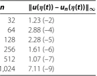
Table 1 The errorsu(η(t)) –un(η(t))∞on boundaryfor Example 1
n u(η(t)) – un(η(t))∞
32 1.23 (–2) 64 2.88 (–4) 128 2.28 (–5) 256 1.61 (–6) 512 1.07 (–7) 1,024 7.11 (–9)
Table 2 Absolute errors|f(z) –fn(z)|at some selected points onfor Example 1
n –1.25 + 0.2i –0.5 + 0.4i 0.5 + 0.4i 1.3 – 0.1i
32 2.10 (–3) 8.0 (–4) 8.0 (–4) 1.30 (–3) 64 2.98 (–5) 6.11 (–5) 6.04 (–5) 3.31 (–5) 128 1.80 (–6) 7.68 (–6) 6.80 (–6) 1.61 (–6) 256 1.99 (–7) 5.79 (–7) 5.10 (–7) 8.08 (–8) 512 1.57 (–8) 5.13 (–8) 3.53 (–8) 4.48 (–9) 1,024 1.15 (–9) 3.32 (–9) 2.39 (–9) 3.08 (–10)
and
β(t) =
⎧ ⎪ ⎨ ⎪ ⎩
(√sint+ ), t∈J,
., t∈J,
.cost, t∈J.
The functionl(t) in () is obtained by choosing an exact solutionu(z) =Re[f(z)], where
f(z) =cos(z) – . This yields the exact valuesc= ,c= .,c= ,c= .,
c= , andc= .. For this example,A(t) =ei(t+cost),t∈J. The integrals in () and () are calculated by the Gauss-Legendre rule with nodes.
Table lists the maximum error normsu(η(t)) –un(η(t))∞, wherenis the number
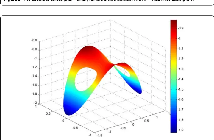
of nodes andun(η(t)) is the numerical approximation ofu(η(t)) based on our method. The errorsf(z) –fn(z)at some selected points are listed in Table . The absolute errors |u(z) –un(z)|for selected points in the entire domain are plotted in Figure . Figure shows the surface plot ofun(z) withn= ,.
Example Consider an unbounded triply connected regionwith boundaries
: η(t) = .cost– .isint,
: η(t) = – + (. + .cost)e–it,
: η(t) = + (. + .cost)e–it, ≤t≤π.
Forα(t) andβ(t) in (), we choose
α(t) =
⎧ ⎪ ⎨ ⎪ ⎩
Figure 3 The absolute errors|u(z) –un(z)|for the entire domain withn= 1,024, for Example 1.
Figure 4 The surface plot ofun(z) for Example 1 withn= 1,024.
and
β(t) =
⎧ ⎪ ⎪ ⎪ ⎨ ⎪ ⎪ ⎪ ⎩
(√ – cost, t∈J
,
|(e–itcost+)i +sinte–it|, t∈J, ((((cost
–
cost
+
cost
) + (sint
+
sint
+
sint
)
))/)/, t∈J .
The functionl(t) in () is obtained by choosing an exact solutionu(z) =Re[f(z)], where
f(z) = z. This yields the exact values,c= ,c= –,c= ,c= .,c= , and
Table 3 The errorsu(η(t)) –un(η(t))∞on boundaryfor Example 2
n u(η(t)) – un(η(t))∞
32 1.38 (–2) 64 9.62 (–4) 128 6.47 (–5) 256 3.87 (–6) 512 4.73 (–7) 1,024 6.57 (–8)
Table 4 Absolute errors|f(z) –fn(z)|at some selected points onfor Example 2
n –0.6 – 0.2i 0.75 0.8 + 0.4i 0.7 + 0.2i
32 7.0 (–4) 4.0 (–4) 1.0 (–3) 1.2 (–3) 64 1.47 (–5) 2.03 (–5) 8.64 (–5) 1.08 (–4) 128 6.51 (–7) 1.87 (–6) 6.51 (–6) 7.95 (–6) 256 2.48 (–7) 6.02 (–7) 4.56 (–7) 5.87 (–7) 512 7.30 (–8) 1.22 (–7) 4.07 (–8) 7.27 (–8) 1,024 1.29 (–8) 1.96 (–8) 5.40 (–9) 1.11 (–8)
Figure 5 The absolute error|u(z) –un(z)|for the entire domain withn= 512, for Example 2.
Table lists the maximum error normsu(η(t)) –un(η(t))∞, wherenis the number
of nodes andun(η(t)) is the numerical approximation ofu(η(t)) based on our method.
The errorsf(z) –fn(z)at some selected points are listed in Table . The absolute errors |u(z) –un(z)|for selected points in the entire domain are plotted in Figure . Figure shows the surface plot ofun(z) withn= .
Example Consider a bounded -multiply connected regionwith boundaries
: η(t) = .cost+ isint,
: η(t) = –. + .i + .e–it,
: η(t) = . + .i + .e–it,
Figure 6 The surface plot ofun(z) for Example 2 withn= 512.
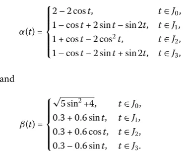
Forα(t) andβ(t) in (), we choose
α(t) =
⎧ ⎪ ⎪ ⎪ ⎨ ⎪ ⎪ ⎪ ⎩
– cost, t∈J,
–cost+ sint–sint, t∈J, +cost– cost, t∈J, –cost– sint+sint, t∈J,
and
β(t) =
⎧ ⎪ ⎪ ⎪ ⎨ ⎪ ⎪ ⎪ ⎩
√
sin+, t∈J, . + .sint, t∈J, . + .cost, t∈J, . – .sint, t∈J.
The functionl(t) in () is obtained by choosing an exact solutionu(z) =Re[f(z)], where
f(z) =z– . This yields the exact values, c
= ,c= –., c= –.,c= .,
c= ., c= ., c = –., and c = .. For this example, A(t) =ei(t–sint),
t∈J. The integrals in () and () are calculated by the Gauss-Legendre rule with nodes.
Table lists the maximum error normsu(η(t)) –un(η(t))∞, wherenis the number
of nodes andun(η(t)) is the numerical approximation ofu(η(t)) based on our method. The errorsf(z) –fn(z)at some selected points are listed in Table . The absolute errors |u(z) –un(z)|for selected points in the entire domain are plotted in Figure . Figure shows the surface plot ofun(z) withn= .
Example Consider an unbounded -multiply connected regionwith boundaries
: η(t) = . +
. + .cos(t)e–it,
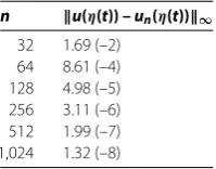
Table 5 The errorsu(η(t)) –un(η(t))∞on boundaryfor Example 3
n u(η(t)) – un(η(t))∞
32 1.69 (–2) 64 8.61 (–4) 128 4.98 (–5) 256 3.11 (–6) 512 1.99 (–7) 1,024 1.32 (–8)
Table 6 The absolute errors|f(z) –fn(z)|at some selected points onfor Example 3
n –1 – 0.2i –0.5 – 0.6i 0.2 + 0.6i 1.2 – 0.3i
32 8.0 (–4) 4.5 (–3) 3.4 (–3) 2.4 (–3) 64 9.10 (–5) 2.24 (–4) 1.48 (–4) 1.10 (–4) 128 6.68 (–6) 1.30 (–5) 8.13 (–6) 6.35 (–6) 256 4.05 (–7) 8.47 (–7) 5.16 (–7) 4.07 (–7) 512 2.33 (–8) 5.63 (–8) 3.46 (–8) 2.69 (–8) 1,024 1.34 (–9) 3.74 (–9) 2.34 (–9) 1.78 (–9)
Figure 7 The absolute error|u(z) –un(z)|for the entire domain withn= 512, for Example 3.
: η(t) = (. + .i) +
.e–it,
: η(t) = (. – .i) + (.cos(t) – .isin(t), ≤t≤π.
Forα(t) andβ(t) in (), we choose
α(t) =
⎧ ⎪ ⎪ ⎪ ⎨ ⎪ ⎪ ⎪ ⎩
– sint, t∈J,
–sint+ cost–sint, t∈J, ( –sint– cost+sint), t∈J,
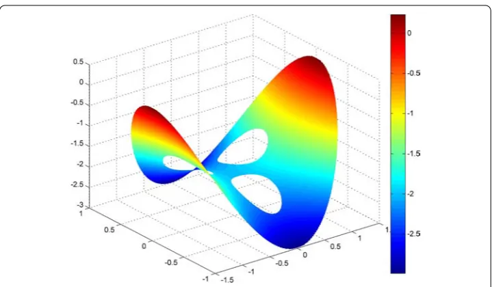
Figure 8 The surface plot ofun(z) for Example 3 withn= 512.
Table 7 The errorsu(η(t)) –un(η(t))∞on boundaryfor Example 4
n u(η(t)) – un(η(t))∞
32 1.56 (–2) 64 8.57 (–4) 128 5.16 (–5) 256 3.21 (–6) 512 1.99 (–7) 1,024 1.24 (–8)
Table 8 The absolute errors|f(z) –fn(z)|at some selected points onfor Example 4
n 0.2 – 0.4i 0.3 – 0.2i 0.6 + 0.2i 1 + 0.5i
32 7.0 (–4) 1.6 (–3) 1.3 (–3) 1.1 (–3) 64 3.87 (–5) 1.02 (–4) 8.92 (–5) 37.07 (–5) 128 2.04 (–6) 6.23 (–6) 5.86 (–6) 4.58 (–6) 256 9.83 (–8) 3.66 (–7) 3.76 (–7) 2.97 (–7) 512 4.34 (–9) 2.12 (–8) 2.39 (–8) 1.92 (–8) 1,024 1.87 (–10) 1.22 (–9) 1.51 (–9) 1.24 (–9)
and
β(t) =
⎧ ⎪ ⎪ ⎪ ⎪ ⎪ ⎪ ⎨ ⎪ ⎪ ⎪ ⎪ ⎪ ⎪ ⎩
((((cost–cost+cost)
+ (sint+sint+sint)))/), t∈J ,
. + .cost, t∈J,
. – .cost, t∈J,
√
sint+ , t∈J.
The functionl(t) in () is obtained by choosing an exact solutionu(z) =Re[f(z)], where
f(z) =z. This yields the exact values,c= ,c= –.,c= ,c= –,c= –.,
Figure 9 The absolute error|u(z) –un(z)|for the entire domain withn= 128, for Example 4.
Figure 10 The surface plot ofun(z) for Example 4 withn= 128.
Table lists the maximum error normsu(η(t)) –un(η(t))∞, wherenis the number
of nodes andun(η(t)) is the numerical approximation ofu(η(t)) based on our method. The errorsf(z) –fn(z)at some selected points are listed in Table . The absolute errors |u(z) –un(z)|for selected points in the entire domain are plotted in Figure . Figure shows the surface plot ofun(z) withn= .
6 Conclusion
and [], the Robin problem has a single boundary condition that is a linear combination of the Dirichlet and Neumann. Here, the method reduces the Robin problem to a RH prob-lem, which leads to a system of integral equations. The proof that these integral equations are linearly independent was shown here. Differential equations were also constructed to provide additional conditions to make the Robin problem uniquely solvable. The integral equations were discretized by the Nyström method with the trapezoidal rule and Wittich’s method, while the differential equations were discretized by the five-point central differ-ence method. The presented numerical results illustrate that the proposed method can be used to produce approximations of high accuracy.
Competing interests
None of the authors have any competing interests in the manuscript.
Authors’ contributions
All authors contributed to the manuscript and typed, read, and approved the final manuscript.
Acknowledgements
The authors would like to thank the editor and referees for their helpful comments and suggestions which improved the presentation of the paper. The authors also would like to thank the Malaysian Ministry of Education and Research Management Centre (RMC), Universiti Teknologi Malaysia for the partial funding through the fundamental research grant scheme (FRGS) vote R.J130000.7809.4F637.
Received: 20 December 2015 Accepted: 26 April 2016 References
1. Heiskanen, W, Moritz, H: Physical Geodesy. Freeman, San Francisco (1966)
2. Fang, W, Suxing, Z: Numerical recovery of Robin boundary from boundary measurements for the Laplace equation. J. Comput. Appl. Math.224, 573-580 (2009). doi:10.1016/j.cam.2008.05.048
3. Gustafson, K, Takehisa, A: The third boundary condition - was it Robin’s? Math. Intell.20(1), 63-71 (1998) 4. Sneddon, IN: Mixed boundary value problems. In: Potential Theory. North-Holland, Amsterdam (1966)
5. Nasser, MMS, Murid, AHM, Ismail, M, Alejaily, EMA: Boundary integral equations with the generalized Neumann kernel for Laplace’s equation in multiply connected regions. Appl. Math. Comput.217, 4710-4727 (2011).
doi:10.1016/j.amc.2010.11.027
6. Alhatemi, SAA, Murid, AHM, Nasser, MMS: Solving a mixed boundary value problem via an integral equation with generalized Neumann kernel on an unbounded multiply connected region. Malaysian J. Fund. Appl. Sci.8(4), 193-197 (2012). doi:10.11113/mjfas.v8n4.147
7. Nasser, MMS: Numerical conformal mapping via a boundary integral equation with the generalized Neumann kernel. SIAM J. Sci. Comput.31, 1695-1715 (2009). doi:10.1137/070711438
8. Wegmann, R, Murid, AHM, Nasser, M: The Riemann-Hilbert problem and the generalized Neumann kernel. J. Comput. Appl. Math.182, 388-415 (2005). doi:10.1016/j.cam.2004.12.019
9. Wegmann, R, Nasser, MMS: The Riemann-Hilbert problem and the generalized Neumann kernel on multiply connected regions. J. Comput. Appl. Math.214, 36-57 (2008). doi:10.1016/j.cam.2007.01.021
10. Petrila, T: Complex value boundary element method for some mixed boundary value problems. Stud. Univ. Babe¸s-Bolyai Inform.44, 37-42 (1999)
11. Mattheij, RMM, Rienstra, SW, ten Thije Boonkkamp, JHM: Partial Differential Equations: Modeling, Analysis, Computation. SIAM, Philadelphia (2005)
12. Howison, S: Practical Applied Mathematics: Modelling, Analysis, Approximation. Cambridge University Press, Cambridge (2005)
13. Kellogg, OD: Foundations of Potential Theory. Ungar, Cambridge (1929)
14. Salsa, S: Partial Differential Equations in Action: From Modeling to Theory. Springer, Milano (2008)
15. Symm, GT: The Robin problem in a multiply-connected domain. In: Brebbia, CA (ed.) Boundary Element Methods in Engineering. Proceedings of the Fourth International Seminar, pp. 89-100. Springer, Berlin (1982)
16. Nasser, MMS: The Riemann-Hilbert problem and the generalized Neumann kernel on an unbounded multiply connected regions. The University Researcher (IBB University Journal)20, 47-60 (2009)
17. Gakhov, FD: Boundary Value Problem. Pergamon Press, Oxford (1966)
18. Hamzah, ASA: Solving Robin Problem Via Integral Equations with the Generalized Neumann Kernel. Master’s Thesis, Universiti Teknologi Malaysia (2013)
19. Atkinson, KE: The Numerical Solution of Integral Equations of the Second Kind. Cambridge University Press, Cambridge (1997)
20. Gaier, D: Konstruktive Methoden der Konformen Abbildung. Springer, Berlin (1965)
21. Abramowitz, M, Stegun, IE: Handbook of Mathematical Functions, with Formulas, Graphs, and Mathematical Tables. Dover, New York (1965)
22. Helsing, J, Ojala, R: On the evaluation of layer potentials close to their sources. J. Comput. Phys.227, 2899-2921 (2008) 23. Swarztrauber, PN: On the numerical solution of the Dirichlet problem for a region of general shape. SIAM J. Numer.