Finding global minimum using filled function method

114

FINDING GLOBAL MINIMUM USING FILLED FUNCTION METHOD

Omar Zahid Bin Ahmad & PM Dr. Rohanin Binti Ahmad

Abstract:

Filled function method is an optimization method for finding global

minimizers. Filled function method is a combination of a local search in findings local

solutions as well as global solution. It is basically a construction and eventually the inclusion

of an auxiliary function called the filled function into the algorithm. Optimizing the objective

function at an initial point will only yield a local minimizer. By using the auxiliary function,

the local minimizer is shifted to a new lower basin of the objective function. The shifted

point is the new initial solution for the local search to find the next local minimizer, where

the function value is lower. The process continued until the global minimizer is achieved.

This research used several test functions to examine the effectiveness of the method in

finding global solution. The results show that this method works successfully and further

research directions are discussed.

Keywords:Optimization, global optimization, local optimization, global minimum, filled

function method

Introduction

The field of optimization has grown rapidly during the past few decades. Many new

theoretical, algorithmic, and computational contributions of optimization have been proposed

to solve various problems in many areas. Recent developments of optimization methods can

be mainly divided into deterministic and heuristic approaches. Deterministic approaches take

advantage of the analytical properties of the problem to generate a sequence of points that

converge to a global optimal solution. Heuristic approaches have been found to be more

flexible and efficient than deterministic approaches; however, the quality of the obtained

solution cannot be guaranteed. Moreover, the probability of finding the global solution

decreases when the problem size increases. Deterministic approaches (e.g., linear

programming, nonlinear programming, and mixed-integer nonlinear programming, etc.) can

provide general tools for solving optimization problems to obtain a global or an

approximately global optimum. With the increasing reliance on modeling optimization

problems in real applications, a number of deterministic methods for optimization problems

have been presented. The study focuses on analyzing the recent advances in deterministic

optimization approaches (Lin, Tsai and Yu, 2012).

Optimization has attracted a great deal of attention from the research community

since many problems arising in many different fields can be posed and solved through

mathematical programming techniques. Interest in optimization intensified in the middle of

20

centuries with the linear programming model which was simple, practical, and perhaps

the only solvable model using the computing power available at the time.

115

Literature Review

In this section, we focus on one FFM that is widely used and become the reference to many

researchers that is

Š

-function, introduced by Renpu Ge in 1990.

Š

, , ½)

=

1/0 + C()5 l2 T

9

W

.

(1)

It was originally put forward by RenpuGe as an effective algorithm of finding global

minimizer of a multi-modal function.

During the year, the theory is raised mainly to cope with unconstrained optimization

problems. The rudimental notion of

filled function

method is: when a local minimizer is

reached, it is hoped that "escaping" this local minimizer is possible. Furthermore, keep

searching, and a better local minimizer is reached. By constructing an auxiliary function, a

local minimizer is shifted into a local maximizer. We make the point perturbed

deterministically, and then, take this perturbed point as the initial point to search, and try to

find the auxiliary function’s local minimizer which is a better local minimizer of the

objective function, or at least as well as the original one (Fang, 2006).

Fang stated that Ge’ FFM is a two-phase iterative: the minimizer phase and the

filling phase. In the first phase, we can use classic minimizer method, such as quasi-Newton

method, the method of steepest descent, etc. to search for a local minimizer

in objective

function. During the second phase, we take the present minimizer as the basic to define a

filled function, and using it to find

′

. Then we take

′

as the starting point and repeat the

first phase. This occurs again and again until the best local minimizer could not be found.

The

filled function method

fully grasps the present local information, for it only applies the

mature local minimizer method, it is greatly popular with the theoretical and practical

operators.

Methodology

An optimization based methods which provide a mechanism to find global solution to the

objective function. A local search is used as a tool to minimize the objective function as well

as the auxiliary function in order to find local minimizer and new initial point respectively.

Which we are already discussed in the literature review. This method provide a ‘jump’ from

one local solution to another local solution until better local called global solution achieved.

This research is concerned with the problem of finding a global minimizer of a twice

continuously differentiable function

C

on

ℝ

. Suppose

C

)

satisfies the condition

C

⟶

∞

as

‖‖

→

+∞

(2)

Then there exists a closed bounded domain

Ω ⊂ ℝ

whose interior contains all global

minimizers of

C()

.

We assume that

Ω

is known and our methods only consider points in

Ω

.

We also assume that

C()

has only a finite number of minimizers in

Ω

and therefore, every

minimizer is an isolated minimizer.

1. Filled Function Method Procedure

116

Phase 1: Finding the local minimizer

We need to find a local minimizer

starting from an initial point and use any local

minimization method such as Newton method.

Phase 2: Finding a new solution in a lower basin

After the local minimum

in the Phase 1 is obtained, then the filled function is

constructed at that point and minimize the filled function in order to identify a point

with

C

(

) C(

)

. If

is formed,

is certainly in a lower basin than

ô

.Use

as an initial point in Phase 1 again.

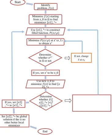
Figure 1

: Procedure flow of the algorithm of filled function method

Start

Identify problem, C()

Minimize C()starting from _0in Ωto find

minimizer 〖1〗_^∗

Use 〖1〗_^∗to construct filled function, Š(,,½)

Minimize Š(,,½)at ̅(l_1) to obtain ′

Determine whether ^′ in Ωor not

If yes, set ′to be _0

Use new _0to minimize C()to find 〖

2〗_^∗

Determine whether C(〖 2〗_^∗ )<C (〖1〗_^∗ ) If yes, set 〖2〗

_^∗to 〖1〗_^∗

Set 〖2〗_^∗be global solution if the is no

other better local minimizer

End

If not, change ̅ at l_!

Increase both ½! and

C(∗) 0 make the ratio

½!_{/( C(}

117

Figure 1 shows the flow chart on the procedure flow that we are concerning in this

research study. The basic idea from Ge (1990) is as follows. At the beginning one may use

any local minimization method. For instance, fminsearch function (Built is used to find a

minimizer

of

C

in the domain

Ω

. Then one attempts to find another minimizer of

C

,

say, which satisfies the inequality

C

≤ C

.

(3)

The idea of finding

!

from

is to fill the basin of

C

at

and other higher

basins of

C

than

ô

so that

is a maximizer of the filled function and the basin

ô

is a

part of a hill of the filled function. Furthermore, the filled function has no minimizers or

saddle points in higher basins of

C

then

ô

, but it does have a "minimizer" along the

direction

in a lower basin of

F(x)

than

ô

if one exists. Thus, one can use an initial

point near

to minimize the filled function. The minimization sequence

leads away

from

and tends to a point

′

which is in a lower basin

ô

of

C

.

Using x' as an initial

point to minimize

F(x),

one can obtain a lower minimizer

of

C

, and so on.

Results and Discussion

In this section, the algorithm is tested on some optimization problems.

(a)

C

2 sin

− sin − 2√

s.t

0 ≤

≤ 6

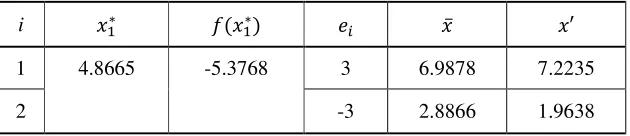
Table 1:

Results of minimizing

Š

-function at

.

i

C

l

̅

′

1

4.8665

-5.3768

3

6.9878

7.2235

2

-3

2.8866

1.9638

From the result tabulated in Table 4.1, the first iteration of minimizing the

Š

-function, the algorithm took the first preset direction,

l

give

7

.

2235

from the first

local minimizer

4

.8665.

This value,

is outside of the

Ω

, so this value is rejected and

continue the algorithm with the next preset direction,

l!

. Eventually, the algorithm arrived at

_{= 1.9638}

_{which in the}

_Ω

_{and then, take it as an initial point to minimize}

_C()

_{, get local}

minimizer

!

1.7251

and the function value

C(!

5

.5677.

Compare the value of

C

(!

_with

_C

∗

. In this case,

C

< C

infact

C

≈ C

, hence the method

arrives at the global minimizer.

From this test, we can see clearly the flow of the algorithm form Phase 1

(minimizing the objective function) to Phase 2 (minimizing the

Š

-function). The process

repeat until the global minimizer found. Thus, the initial testing for the algorithm is quite

successful. Next, the algorithm is tested with higher number of local minima problem.

(b)

C sin sin

2 − cos 4

s. t − 2 ≤ ≤ 4.

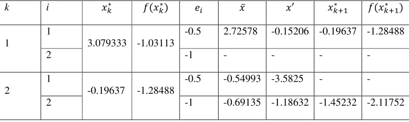
118

k

i

7

C

l

̅

′

C

1

1

3.079333 -1.03113

-0.5

2.72578

-0.15206 -0.19637 -1.28488

2

-1

-

-

-

-

2

1

-0.19637

-1.28488

-0.5

-0.54993 -3.5825

-

-

2

-1

-0.69135 -1.18632 -1.45232 -2.11752

The result shows that the algorithm able to find another new local minimizer in

lower basin from the previous local minimizer. This confirmed that the algorithm continues

to run until there is no local minimizer found anymore.

Noted that, the use of preset directions,

l

are different from problem (a) with

problem (b). It is define differently according to the problem as well as the parameters

½

and

C

. Though the value of the parameter need to be chose and adjust until the global

solution come out from the algorithm. The preset direction also taking as important part as it

take role as movement of the

Š

-function in finding the

′

.

Table 3 :

Result of minimizing Problem (4.2) at different value of parameter

½

.

From table above, at different value of

½

, that is

½

0.5

, the computing of the

algorithm will arrive at local minimizer of

b

basin. The result is then,

C

(!

≥

C

which

means the algorithm had through Step 7 as in the algorithm in Section 3.5. The value of

½

is

increased so that the ratio

½

/0 C

5

becomes small.

According to Ge (1990), the reasons for obtaining

C

≥

C

are either the ratio

½

_{/0 C}

∗

5

is not small enough or

‖

‖

is too large so that the computer cannot

recognize the change of

Š

, , ½)

.

Therefore, the both

½

and

[ C(

5

need to be

increase to make the ratio

½

/0 C

5

smaller than the previous one as in Step 7 (refer to

FFM algorithm in Section 3.5). Do not only decrease

½

to decrease the ratio

½

/0 C

5

because too small

½

makes the filled function descend very quickly when

is close to

but very slowly when

is a little bit further from

and therefore some difficulty arises in

the minimization process of

Š

, , ½)

.

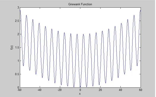
(c)

G

riewank

∑

∏

cos T

√M

W

1

% Mä

−600 ≤

≤ 600

for ¥

1, … , 4.

k

7

C

′

C

1

3.07933

-1.03113

1.38627

1.70618

-0.13354

2

1.70618

-0.13354

1.04766

1.70618

-0.13354

-

-

0.64132

-0.19634

-1.28488

119

The global minimum value is 0 and the global is located in the origin, but the

function also has a very large number of local minima, exponentially increasing

with

4

.

Figure 3 :

Graph of Griewank function

Table 4 :

Result of minimizing the Griewank function

k

7

C

̅

′

C

1

50.24036

0.631339

46.70483

46.55751

43.96031

0.483369

2

43.96031

0.483369

40.42478

40.27747

37.68027

0.355128

3

37.68027

0.355128

33.99742

33.99742

31.40023

0.246617

4

31.40023

0.246617

27.86469

27.71738

25.12018

0.157835

5

25.12018

0.157835

21.58465

21.43733

18.84014

0.088782

6

18.84014

0.088782

15.30460

15.15729

12.56009

0.039459

7

12.56009

0.039459

9.02456

8.877243

6.280046

0.009865

8

6.280046

0.009865

2.74451

2.597197

0.0000

0.0000

For the simulation, first, the initial points is chose within the box-constraint

600 ≤

M

≤ 600

, and the parameters of the FFM that are

C(

3

and

½ =

1

be fixed as well

120

Conclusion

Filled function method (FFM) by Ge’s provided a better mechanism in finding global

solution for global optimization problem. Whereas, the conventional optimization method

such as Newton’s Method incapable finding the global but local optima only. Though, the

FFM combined with the conventional optimization method in the algorithm for this to work

together with its auxiliary function that is

Š

-function.

However, Ge’s FFM had several drawbacks in his algorithm which become a field to

explore for other researchers. There are two major drawbacks that many researchers

eventually take into consideration. First, there are two adjustable parameters,

and

½

,

which greatly affect the performance of the algorithms and need to be appropriately adjusted.

However, how to adjust the parameters is a very difficult task. Second, the filled functions

are likely to be ill-conditioned in practice since their function values increase exponentially

due to an exponential function. As the adjustable parameter becomes larger and larger, which

is required by the FFM itself, the rapidly increasing exponential function value may result in

an overflow in the computation (Wei, Wang and Shang, 2013).

References

Ge, R. P. (1990). A filled function method for finding a global minimizer of a function of

several variables.

Mathematical Programming

. Vol. 46, no. 2, pp. 191–204.

Bector, C.R., Chandra, S., and Dutta, J. (2004).

Principles of the Optimization Theory

. New

Delhi: Narosa Publishers.

Lin, M. H., Tsai, J. F., and Yu, C. S. (2012). A Review of Deterministic Optimization

Methods in Engineering and Management.

Mathematical Problems in Engineering,

Volume

2012, Article ID 756023. Creative Commons Attribution License.

Pardalos, P. M., and Romeijin, H. E. (2002).

Handbook of Global Optimization: Nonconvex

Optimization and Its Applicaton

(vol 2). Netherlands: Kluwer Academics Publishers

Horst, R., and Tuy, H., (1996).

Global Optimization: Deterministic Approaches

(3

ed.).

New York: Springer-Verlag

121

to Global Optimization

. Cambridge:MIT

Wang, W., Shang, Y., and Zhang, L. (2007). A filled function method with one parameter

for

box constrained global optimization.

Applied Mathematics and Computation

.Vol. 194, no. 1,

pp. 54–66.

Zhang, Y., Zhang, L., and Xu, Y. (2009). New filled functions for nonsmooth global

optimization.

Applied Mathematical Modelling

. Vol. 33, no. 7, pp. 3114–3129.

Levy, A. and Montalvo, A. (1985). The tunneling algorithm for the global minimization of

the functions. SIAM J. Sci. Stat. Comput. 6(1) 15-29.

Lin, H., Wang, Y., and Fan, L. (2011). A filled function method with one parameter for

unconstrained global optimization.

Applied Mathematics and Computation

. Vol. 218, no. 7,

pp. 3776–3785.

Liu, X. and W. Xu (2004). A new filled function applied to global optimization.

Computers

& Operations Research

31

(1): 61-80.

Snyman, J. A., and Fatti, L. P. (1987). A Multi-Start Global Minimization Algorithm with

Dynamic Search Trajectories.

Journal Of Optimization and Applications.

Vol. 54, no. 1, pp.

122-141.

Birbil S. I. and. Fang, S.-C. (2003). An electromagnetism-like mechanism for global

optimization.

Journal of Global Optimization

. Vol. 25, no. 3, pp. 263–282.

P. M. Pardalos, H. E. Romeijn, and H. Tuy. ( 2000). Recent developments and trends in

122

pp. 209–228.

Romeijn, H.E. and Smith, R.L. (1994). Simulated Annealing for Constrained Global

Optimization.

Journal of Global Optimization

. Vol. 5, pp. 101–126

Cvijović, D. and Klinowski J. (1995). Taboo search: an approach to the multiple minima

problem Science, Vol. 267, pp. 664–666

Glover, F. and Laguna, M. (1997).

Tabu Search

. Boston, MA: Kluwer Academic Publishers.

Diener, I. (1987). Trajectory Methods in Global Optimization.

Handbook of Global

Optimization.

Vol 2, no. 1, pp. 649-667.

Locatelli, M. (2003). A Note on the Griewank Test Fucntion.

Journal of Global

Optimization.