Classification and Predictability of the Western Boundary Current Instabilities in the Gulf of Mexico and South Atlantic Bight

ABSTRACT

ZENG, XIANGMING. Classification and Predictability of the Western Boundary Current Variability in the Gulf of Mexico and South Atlantic Bight. (Under the direction of Dr. Ruoying He).

Many instabilities exist in the western boundary current system in the North Atlantic, such as path shifts, meanders and eddy shedding. Regional climate systems, local weather systems and marine ecosystems can be significantly affected by these instabilities. Using state-of-art methods, this dissertation explores different patterns, predictability, and mechanisms of two major components of the Western Boundary Current system in the North Atlantic: the Loop Current (LC) in the Gulf of Mexico (GoM) and the Gulf Stream (GS) in the South Atlantic Bight (SAB).

First, variations of the LC in the GoM are investigated using over two decades of satellite altimeter data and the self-organizing map method. It is found that LC variations can be characterized by three spatial patterns: normal, extension and retraction. The corresponding temporal variations confirm that LC eddy shedding generally occurs during the transition from the extension to retraction patterns. On the weekly time scale, the wind stress curl (WSC) in the Caribbean Sea has a major influence on LC eddy shedding. The increase of Caribbean WSC from June to November favors more frequent LC eddy shedding during that period. On the interannual time scale, there is a potential linkage between the frequency of LC eddy shedding and El Niño activities.

satellite-observed SSH into spatial patterns (EOFs) and time-dependent principal components (PCs). Then the nonlinear autoregressive neural network is developed to predict major PCs of the GoM SSH in the future. The prediction of SSH in the GoM is subsequently constructed by multiplying the EOFs and predicted PCs. Validations against independent satellite observations indicate that the neural network–based model can reliably predict the LC variations and its eddy shedding process for a 4-week period. In some cases, an accurate forecast for 5–6 weeks is possible.

Classification and Predictability of the Western Boundary Current Instabilities in the Gulf of Mexico and South Atlantic Bight

by

Xiangming Zeng

A dissertation submitted to the Graduate Faculty of North Carolina State University

in partial fulfillment of the requirements for the degree of

Doctor of Philosophy

Marine, Earth, and Atmospheric Sciences

Raleigh, North Carolina 2016

APPROVED BY:

_______________________________ Dr. Ruoying He

Chair of Advisory Committee

_______________________________ _______________________________ Dr. John Bane Dr. Ping-Tung Shaw

i

DEDICATION

ii

BIOGRAPHY

Xiangming Zeng was born and raised in a small village in Shandong, China. He received his bachelor degree in Mathematics in 2007 at Ocean University of China and master degree in Physical Oceanography in 2010 at Second Institute of Oceanography, China State Oceanic Administration. After working two years as a research associate in the same institute, he joined the Department of Marine, Earth, and Atmospheric Sciences at North Carolina State University in August 2012 to start his doctoral study.

Xiangming are very interested in using data and models to solve real world problems. He loves the elegant math behind models and fascinating ideas of exploring and explaining data. He’d like to use what he has learned to make the world a better place.

iii

ACKNOWLEDGMENTS

I would like to thank my advisor, Dr. Ruoying He, for his continuous support of my Ph.D. research. I am very grateful to my committee: Dr. Ruoying He, Dr. John Bane, Dr. Ping-Tung Shaw, Dr. Fredrick Semazzi, and Dr. Nagiza Samatova, for their valuable guidance and suggestions. I would also like to thank all the current and past members of Ocean Modeling and Observing Group, Ms. Jennifer Warrillow, Dr. Joseph Zambon, Dr. Jeffrey Willison, Dr. Benjamin Johnson, Dr. Yanlin Gong, Dr. Haibo Zong, Ms. Laura McGee, Dr. Ke Che, Dr. Yizhen Li, Dr. Ping Zhai, Dr. Austin Todd, Dr. Yi Xu, Dr. Zhiren Wang, Dr. Zhigang Yao, Dr. Zuo Xue, Dr. Yuqi Yin, Dr. Chuanjun Du, Dr. Hui Qian, and others who gave me a lot of help during my Ph.D. study. Many thanks to the faculties, staffs, and friends in the Department of Marine, Earth, and Atmospheric Sciences, especially Dr. Paul Liu, Dr. Bin Liu, Xiaoyu Long, Yao Wang, Doreen McVeigh, and many other friends in my life, who made my life more colorful.

iv

TABLE OF CONTENTS

LIST OF TABLES ... vii

LIST OF FIGURES ... viii

Chapter I: Introduction ... 1

1. Western Boundary Current instabilities ... 1

2. Loop Current in the Gulf of Mexico ... 2

3. Gulf Stream in the South Atlantic Bight ... 4

4. Research objectives and dissertation outline ... 7

References ... 9

Figures ... 15

Chapter II: Clustering of Loop Current patterns based on the satellite-observed sea surface height and self-organizing map ... 17

Abstract ... 18

1. Introduction ... 18

2. Data and methods ... 20

3. Results ... 21

3.1 Spatial variability ... 22

3.2 Temporal evolution ... 22

4. Discussion ... 23

5. Summary ... 25

Acknowledgement ... 26

References ... 27

Figures ... 31

Chapter III: Predictability of the Loop Current variation and eddy shedding process in the Gulf of Mexico using an artificial neural network approach ... 35

Abstract ... 36

1. Introduction ... 36

v

2.1 Dataset ... 39

2.2 Artificial neural network (ANN) ... 40

2.3 EOF analysis ... 41

2.4 Prediction Procedure ... 42

3. Results and discussion ... 45

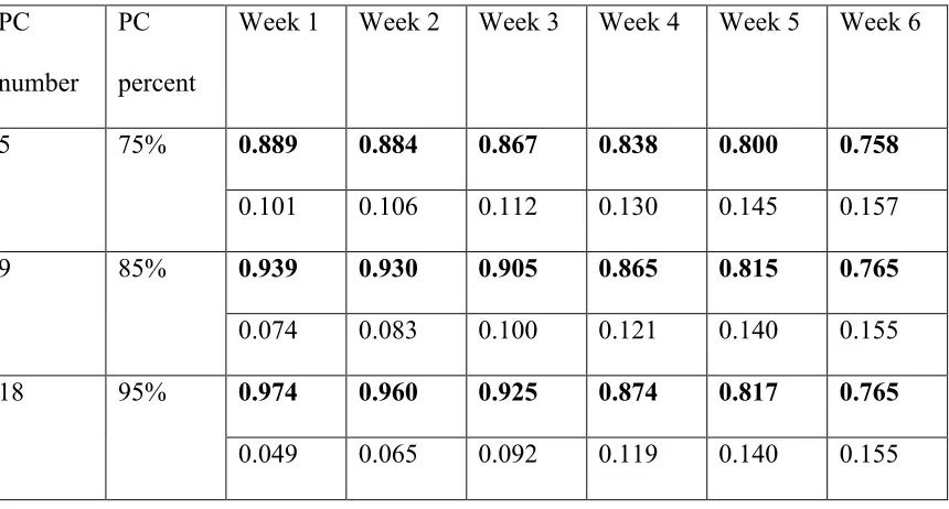
3.1 Sensitivity of PC number selection ... 45

3.2 SSH prediction skill assessment ... 46

3.3 Frontal position prediction skill assessment ... 49

3.4 One LC eddy shedding example ... 51

4. Summary ... 52

Acknowledgement ... 54

References ... 54

Tables ... 61

Figures ... 62

Chapter IV: Gulf Stream variability and a triggering mechanism of its large meander in the South Atlantic Bight ... 76

Abstract ... 77

1. Introduction ... 77

2. Gulf Stream path variation over the last two decades ... 80

2.1 Gulf Stream path detection ... 80

2.2 Self-Organizing Map analysis ... 82

3. Triggering mechanism analysis ... 84

3.1 Ocean model configuration and validation ... 84

3.2 Adjoint sensitivity model ... 86

3.3 Forward model results ... 90

3.4 Validity of tangent linear assumption and index function definition ... 92

3.5 Adjoint sensitivity analysis ... 94

4. Barotropic vorticity budget ... 96

vi

Acknowledgement ... 100

References ... 101

Figures ... 109

vii

LIST OF TABLES

viii

LIST OF FIGURES

Chapter I

Figure 1. (a) Eddy kinetic energy (m2/s2) derived from 21 years’ mean AVISO sea level anomaly satellite data. (b) Study domain. Black arrows are geostrophic currents (> 0.1 m/s) derived from 21 years’ mean AVISO sea surface height data. They can be considered to be part of the Western Boundary Current system in the North Atlantic. Contours are isobaths at 100, 1000, and 3000 m. ... 15  

Figure 2. Topography of the South Atlantic Bight. Water depth is shown in meters. Contours are 200, 600, 700, 1000, and 3000 m isobaths. The Charleston Bump is shown by the arrow. ... 16  

Chapter II

Figure 1. Study domain. Red box is the Gulf of Mexico (GoM) area; blue box is the Caribbean Sea (CS) area; green box is the Bahamas area. The box areas are used for wind stress curl calculations. Grey lines are depth contours in meters. Black arrows are geostrophic velocity calculated from long-term mean AVISO sea surface height data (only the velocities >0.1 m s-1 _{are plotted). The Loop Current is visible via the velocity}

arrows in the GoM box. ... 31  

Figure 2. Self-organizing map analysis results. (a) Sea surface height (SSH) patterns: (P1) normal; (P2) extension; (P3) retraction. Top numbers are corresponding frequency of occurrence (FO) percentage. Vectors are geostrophic current. Green line is 0.45 m SSH contour line. Cyan lines are 1000 m isobaths. Color scale: SSH in meters. (b) Best matching unit (BMU) time series of the three patterns in (a). Red stars are the first day of each year. (c) Monthly FOs of the three patterns in (a). ... 33  

ix Chapter III

Figure 1. Study domain. Black box is study area in the Gulf of Mexico (GoM). Stars are the seven reference stations for frontal position comparison. Grey lines are depth contours in meters. Black arrows are geostrophic velocity calculated from long-term mean AVISO sea surface height data (only the velocities >0.1 m/s are plotted). The Loop Current is visible via the velocity arrows in the GoM box. Dash lines are tracks of hurricanes or tropical storms (TS) from July 2010 to July 2013. 1: TS Bonnie, July 22-25, 2010; 2: Hurricane Paula during October 11-15, 2010; 3: TS Don, July 27-30, 2011; 4: Hurricane Rina, October 22-29, 2011; 5: TS Debby, June 23-27, 2012; 6: Hurricane Ernesto, August 1-10, 2012; 7: Hurricane Isaac, August 20-30, 2012; 8: TS Andrea, June 5-10, 2013. The tracks of hurricanes and tropical storms are from NOAA National Climatic Data Center and The Johns Hopkins University Applied Physics Laboratory. 62  

Figure 2. Comparison between predicted (circles) and observation-derived (stars) first leading principal component of GoM SSH from 2010 to 2013. Correlation coefficients are presented at the top of each figure. ... 64  

Figure 3. Spatial correlation coefficients (CC) and root mean square errors (RMSE) of predicted and observed sea surface height in the study area from 2010 to 2013 with a six-week ahead weekly sliding prediction window, using 18 PCs. Circles are CC points, and triangles are RMSE points. Red lines in week 6 indicate the approximate passing time of Hurricane Rina in 2011, Hurricane Ernesto in 2012, and Tropical Storm Andrea in 2013. ... 66  

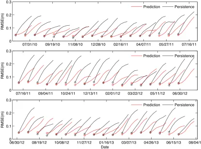
Figure 4. Root Mean Square Error (RMSE) comparison of sea surface height between prediction (red) and persistence (black). Circles represent the location of week 1. The values are plotted every four weeks. ... 67  

Figure 5. Averaged Root Mean Square Error (RMSE) of sea surface height for prediction (red) and persistence (grey). Thin lines are monthly means, and thick lines are means over the three-year prediction period. ... 68  

x

Figure 7. Averaged skill score of sea surface height for prediction (red) and persistence (grey). Thin lines are monthly mean, and thick lines are means over the three-year prediction period. ... 70  

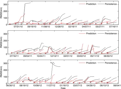
Figure 8. Frontal position Root Mean Square Error (RMSE) comparison of Loop Current and Loop Current eddies between prediction (red) and persistence (black). Circles represent the location of Week 1. The values are plotted every four weeks. ... 71  

Figure 9. Averaged frontal position Root Mean Square Error (RMSE) for prediction (red) and persistence (grey). The sudden jumps in Figure 8 were excluded when the average was calculated. Thin lines are monthly means, and thick lines are means over the three-year period. ... 72  

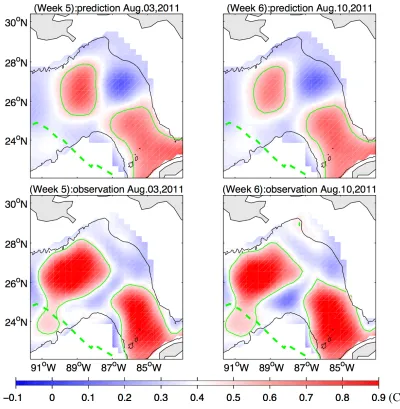
Figure 10. Comparison between forecasted and observed sea surface height in week 1-2 (panel A), week 3-4 (panel B), week 5-6 (panel C), representing a complete cycle of one Loop Current (LC) eddy shedding event. Black lines are 1000 m isobaths. Red areas are the LC and LC eddies. Green solid lines are 0.45 m contours for observation, and 0.51 m contours for prediction. Green dashed lines are the track of Tropical Storm Don during July 27-30, 2011. ... 75  

Chapter IV

Figure 1. Model domain. Black arrows are geostrophic currents (> 0.1 m/s) derived from 21 years of mean AVISO Absolute Dynamic Topography data. They can be considered as the western boundary current system in the North Atlantic. Contours are 100, 1000, and 3000 m isobaths. ... 109  

Figure 2. Topography of the South Atlantic Bight. Water depth is shown in meters and extracted from the 1-minute GEBCO dataset. The Charleston Bump is indicated. ... 110  

Figure 3. Long-term (1993-2013) mean Absolute Dynamic Topography (ADT, color shading, unit: m) overlaid with Gulf Stream mean path (solid black curve) and corresponding envelope (dashed cyan curves) and one standard deviation (STD, dashed black curves). Transects 1 to 5 (solid lines perpendicular to the Gulf Stream mean path) were used to measure the position variation of the Gulf Stream. Gray contours are 200, 600, 1000, and 2000 m isobaths. Black box is for the index function definition in section 3. Florida (FL) and the Charleston Bump are indicated. ... 111  

xi

shaded region indicates the largest offshore event in 2009-2010. A 30-day low-pass filter was applied to the original data for visualization purpose. ... 113  

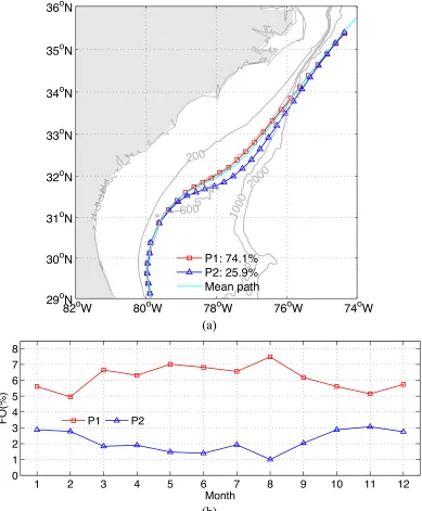
Figure 5. Self-Organizing Map analysis of the Gulf Stream path in the South Atlantic Bight. (a) Weakly (P1) and strongly (P2) deflected patterns. The numbers are corresponding frequency of occurrence (FO) for each pattern. The mean path is indicated by the cyan curve. (b) Monthly FOs of the two patterns in (a). ... 114  

Figure 6. Comparisons between Florida Current (FC) transport and monthly FO of strongly deflected pattern (P2). (a) Monthly mean FC transport (Sv) and FO of P2 (%). Correlation coefficient is -0.81. (b) Monthly standard deviation (STD) of FC transport (Sv) and FO of P2 (%). Correlation coefficient is 0.66. ... 115  

Figure 7. Observed (blue) and simulated (red) daily sea level at three stations (a, b, and c) along the SAB, and water transport through the Florida Straits (d). Sea level data are normalized (minus mean divided by the corresponding standard deviation). Locations of the three stations and the FC transect is shown in Figure 8a. ... 117  

Figure 8. Simulated surface velocity (vectors) and relative vorticity (color shading) from Nov. 17 to 26, 2009, every three days. Relative vorticity is normalized by dividing by the Coriolis parameter. Black stars in (a) indicate the location of the three sea level stations, and black hexagon represents Abaco Island. Purple solid line in (a) represents the location of the cable measuring the Florida Current (FC) transport. Black box (same as the one in Figure 3) delineates the region for index function calculation. Gray lines are the 200, 600, 1000, and 2000 m isobaths. The purple, red, and yellow transects in (a) are sites where water transport was calculated for the FC, Antilles Current, and Gulf Stream, respectively. ... 118  

Figure 9. Simulated water transport through the three transects in Figure 8a. These indicate the water transport of Florida Current, Antilles Current, and Gulf Stream. ... 119  

Figure 10. Comparisons between the nonlinear perturbation runs and tangent linear model solutions in terms of sea surface height (SSH) and velocity (u and v). Gray lines represent the 50 perturbation experiments, and solid black lines are the corresponding mean. ... 120  

xii

The dashed rectangular box indicates the time window for adjoint sensitivity analysis. ... 121  

Figure 12. Adjoint sensitivity to depth-averaged velocity. Vectors represent direction. Color indicates magnitude (unit: 1/s). Gray lines are the 200, 600, 1000, and 2000 m isobaths. Black boxes are the region for index function calculation. ... 122  

Figure 13. Schematics of positive relative vorticity perturbation formation. Orange circles with plus signs indicate positive relative vorticity. Blue circles with minus signs represent negative relative voracity. Vectors are velocity fields. Shaded ellipse represents the Charleston Bump. ... 123  

Figure 14. Ten-day (Nov. 17-26, 2009) averaged tendency, planetary vorticity advection (BETA), bottom pressure torque (BPT), and nonlinear advection (ADV) terms in the barotropic vorticity equation (unit: m/s2). Gray lines are the 200, 600, 1000, and 2000 m isobaths. Cyan lines are the 1, 21, and 41 Sv batrotropic streamlines (integrated from coastlines). Green boxes define the region for the time series plot in Figure 16. Black boxes indicate the region for the index function calculation. ... 124  

1

Chapter I: Introduction

1. Western Boundary Current instabilities

Some of the most prominent features of ocean circulation are the strong, persistent currents along the western boundaries of ocean basins, which are known as Western Boundary Currents (WBCs), such as the Gulf Stream in the Atlantic and Kuroshio Current in the Pacific. The formation of WBCs is mainly due to the beta effect of the Coriolis force varying with latitude (Stommel 1948). Originating from the equatorial regions, WBCs carry warm water from low to high latitudes, thus not only affecting the local circulation and marine ecosystem, but also contributing to the global meridional heat transport and moderation of Earth’s climate (Imawaki et al. 2013).

2

weather systems (e.g. Minobe et al. 2010), or can be indicators of global climate variations (e.g. Wu et al. 2012).

Instabilities of WBC systems usually result in meanders and eddy shedding, and consequently, high eddy kinetic energy (EKE). Figure 1a shows the distribution of climatological means EKE in the North Atlantic, estimated from 21 years of satellite-observed sea level anomaly data. As expected, high EKE occurs near the WBC region with large instabilities (Figure 1b). The greatest EKE in Figure 1a is located in the open ocean region where the Gulf Stream veers away from the coastline to the east. Much studies have been done on the part of Gulf Stream and its interaction with topography and Atlantic Ocean circulation. In this study, I will focus on two of its upstream regions: the Gulf of Mexico and the South Atlantic Bight, where significant EKE are also observed.

2. Loop Current in the Gulf of Mexico

3

irregular, ranging from 0.5 to 18 months (Leben 2005). Between eddy shedding, variations of LC frontal position are also significant. The north and west edges of the LC can vary from about 25.5°N to 27.5°N and 86°W to 90°W, respectively (Leben 2005; Gopalakrishnan et al. 2013).

Daily operations of approximately 4,000 oil and gas drilling platforms in the northern GoM are significantly affected by the LC and its high-speed eddies, which make planning and scheduling a challenge for this expensive enterprise (Leben and Honaker 2006; Sammarco et al. 2004). Accurate prediction of the LC and LC eddies is of critical importance for both scientific research and societal benefit. For example, in order to mitigate the adverse impacts of the Deepwater Horizon oil spill in 2010, intensive research on the LC and LC eddies was performed during and after the incident (e.g., Liu et al. 2013). The LC and LC eddies also play an active role in the rapid intensification of GoM hurricanes, such as devastating Hurricanes Katrina and Rita (Leben and Honaker 2006), which caused extensive loss of life and property damage in many Gulf coastal communities.

4

latitude and eddy separation period. Forristall et al. (2010) showed that of statistical methods have better skills on LC prediction than that of most dynamical models. Mooers et al. (2012) evaluated several different ocean models’ performances at LC eddy shedding prediction using various prediction skill assessment methods in the report of the GoM 3-D Operational Ocean Forecast System Pilot Prediction Project. More recently, with the four-dimensional variation method, Gopalakrishnan et al. (2013) tested the predictability of the LC eddy shedding process using the Massachusetts Institute of Technology general circulation model (MITgcm). Xu et al. (2013) applied the local ensemble transform Kalman filter with the parallel POM to estimate the states of the LC and LC eddies from April to July 2010.

All the above studies are based on either simple empirical relations or primitive equation ocean models focusing on a single LC eddy or a small number of LC eddy shedding events. The lack of generality makes the assessment of their model predictability very difficult (e.g., Mooers et al. 2012). As a powerful tool in many areas, such as pattern recognition, parameter optimization, and time series prediction, the machine learning technique will be used to analyze and predict variations of the LC and LC eddies.

3. Gulf Stream in the South Atlantic Bight

5

trough bottom structure off Charleston, SC, known as the “Charleston Bump” (Bane and Brooks 1979; Figure 2). The offshore deflection of the GS usually propagates downstream of the Bump, which can even affect the position of the GS near Cape Hatteras.

The position of the GS can affect the coastal circulation, along- and cross-shelf water exchange, marine ecosystem, and regional weather system in the SAB. For instance, Miller and Lee (1995) shows as the GS flows along the shelf break of the SAB, the variation of its position can easily change the circulation on the continental shelf. Frontal eddies and water intrusion caused by the instability and variation of the GS play an important role in the water exchange between continental shelf and the open ocean (Lee et al. 1991; Castelao 2011). At the same time, these processes can also transport nutrients to the euphotic zone beneath the GS, which further affects productivity and biomass variation in the SAB (Lee et al. 1991; Signorini and McClain 2007). Because of the influence of hydrodynamics on fisheries, fish population and larval transport in the SAB are closely linked to the position of the GS (Werner et al. 1997; Epifanio and Garvine 2001). Furthermore, GS position can impact the distribution of sea surface temperature, which moderates the ocean-to-atmosphere heat fluxes and results in variation of the local weather system (Bane and Osgood 1989; Li et al. 2002; Joyce et al. 2009; Kwon et al. 2010; Minobe et al. 2010; Nelson et al. 2014).

6

7

interactions of the GS with topographic features and the subsequent impact of nonlinear eddy-mean flow interactions through a high-resolution model.

Because of limited observations, the understanding of GS path variability over a longer time scale is very limited. With the continued development of satellite altimetry and new ocean modeling and adjoint sensitivity tools, it is now possible to use two decades’ satellite observed sea surface height data and quantitative model simulation results to explore the long-term variation of the GS path and elucidate the mechanisms that determine such variation.

4. Research objectives and dissertation outline

The overarching objective of this dissertation research is to achieve a deeper understanding of the patterns, mechanisms, and predictability of WBC system variation in the GoM and the SAB using the state-of-art data analysis and numerical model diagnostic methods. Specific objectives are:

I.   Extract the pattern and evolution of LC and LC eddies in the GoM by clustering the corresponding satellite-observed sea level data over two decades (1992-2013). Identify possible environmental factors that affect the state of the LC.

II.   Explore the predictability of LC state using a new machine learning forecasting method and provide a comprehensive assessment on the prediction skills of this method.

8

IV.  Identify dynamical mechanisms that cause variation of GS position using realistic ocean hindcast and adjoint models.

The outline of this dissertation is as follows: Chapter II focuses on the clustering of the LC patterns based on the satellite altimeter data. Different patterns of the LC are extracted from long-term satellite observation. The influence of wind stress and climate variation on the LC temporal variation is explored. Based on the analysis in Chapter II, a forecasting system is developed to predict the state of the LC and LC eddies in Chapter III. Validations against independent satellite observations are also provided. Chapter V focuses on the GS in the SAB. First, the long-term GS position variability is quantified using two decades’ satellite altimeter data. Factors that may affect the GS position in the SAB are analyzed from statistical point of view. Then, a realistic ocean circulation model is developed to simulate the GS offshore meanders in November 2009. This meander kept evolving in the next 4-5 months, constituting the largest offshore meander event over last two decades. Triggering mechanisms of this meander in November are studied using the adjoint sensitivity and vorticity budget analysis methods. Finally, a summary of this dissertation is presented in Chapter IV.

9 References

Bane, J. M. (1983), Initial observations of the subsurface structure and short-term variability of the seaward deflection of the Gulf Stream off Charleston, South Carolina, J. Geophys. Res., 88(C8), 4673–4684, doi:10.1029/JC088iC08p04673.

Bane, J. M., and D. A. Brooks (1979), Gulf Stream meanders along the Continental Margin from the Florida Straits to Cape Hatteras, Geophys. Res. Lett., 6(4), 280–282, doi:10.1029/GL006i004p00280.

Bane, J. M., and W. K. Dewar (1988), Gulf Stream bimodality and variability downstream of the Charleston bump, J. Geophys. Res., 93(C6), 6695–6710, doi:10.1029/JC093iC06p06695.

Bane, J. M., and K. E. Osgood (1989), Wintertime air-sea interaction processes across the Gulf Stream, J. Geophys. Res., 94(C8), 10755–10772, doi:10.1029/JC094iC08p10755. Bane, J. M., D. A. Brooks, and K. R. Lorenson (1981), Synoptic observations of the

three-dimensional structure and propagation of Gulf Stream meanders along the Carolina continental margin, J. Geophys. Res., 86(C7), 6411–6425, doi:10.1029/JC086iC07p06411.

Castelao, R. (2011), Intrusions of Gulf Stream waters onto the South Atlantic Bight shelf, J. Geophys. Res., 116(C10), C10011, doi:10.1029/2011JC007178.

Castelao, R. M., and R. He (2013), Mesoscale eddies in the South Atlantic Bight, J. Geophys. Res. Oceans, 118(10), 5720–5731, doi:10.1002/jgrc.20415.

Counillon, F., and L. Bertino (2009), High-resolution ensemble forecasting for the Gulf of Mexico eddies and fronts, Ocean Dynamics, 59, 83–95, doi:10.1007/s10236-008-0167-0.

Cushman-Roisin, B., and J.-M. Beckers (2011), Introduction to Geophysical Fluid Dynamics: Physical and Numerical Aspects, Academic Press.

10

Forristall, G. Z., R. R. Leben, and C. A. Hall (2010), A Statistical Hindcast and Forecast Model for the Loop Current, Offshort Technologyh Conference, doi:doi:10.4043/20602-MS.

Fuglister, F. C., and A. D. Voorhis (1965), A New Method of Tracking the Gulf Stream,

Limnol. Oceanogr., 10(suppl), R115–R124, doi:10.4319/lo.1965.10.suppl2.r115.

Gawarkiewicz, G. G., R. E. Todd, A. J. Plueddemann, M. Andres, and J. P. Manning (2012), Direct interaction between the Gulf Stream and the shelfbreak south of New England,

Sci. Rep., 2, doi:10.1038/srep00553.

Gopalakrishnan, G., B. D. Cornuelle, and I. Hoteit (2013), Adjoint sensitivity studies of loop current and eddy shedding in the Gulf of Mexico, Journal of Geophysical Research: Oceans, n/a–n/a, doi:10.1002/jgrc.20240.

Gula, J., M. J. Molemaker, and J. C. McWilliams (2014), Gulf Stream dynamics along the Southeastern U.S. Seaboard, J. Phys. Oceanogr., doi:10.1175/JPO-D-14-0154.1.

Hogg, N. G., and W. E. Johns (1995), Western boundary currents, Rev. Geophys., 33(S2), 1311–1334, doi:10.1029/95RG00491.

Hsieh, W. W. (2001), Nonlinear principal component analysis by neural networks, Tellus A,

53(5), 599–615, doi:10.1034/j.1600-0870.2001.00251.x.

Imawaki, S., A. S. Bower, L. Beal, and B. Qiu (2013), Western Boundary Currents, in Ocean Circulation and Climate - A 21st Century Perspective, 2nd Edition, pp. 305–338, Academic Press.

Ishikawa, Y., T. Awaji, N. Komori, and T. Toyoda (2004), Application of Sensitivity Analysis Using an Adjoint Model for Short-Range Forecasts of the Kuroshio Path South of Japan, Journal of Oceanography, 60(2), 293–301, doi:10.1023/B:JOCE.0000038335.50080.ff.

Joyce, T. M., Y.-O. Kwon, and L. Yu (2009), On the Relationship between Synoptic Wintertime Atmospheric Variability and Path Shifts in the Gulf Stream and the Kuroshio Extension, J. Climate, 22(12), 3177–3192, doi:10.1175/2008JCLI2690.1. Kwon, Y.-O., M. A. Alexander, N. A. Bond, C. Frankignoul, H. Nakamura, B. Qiu, and L. A.

Large-11

Scale Atmosphere–Ocean Interaction: A Review, J. Climate, 23(12), 3249–3281, doi:10.1175/2010JCLI3343.1.

Leben, R. R. (2005), Altimeter-Derived Loop Current Metrics, in Circulation in the Gulf of Mexico: Observations and Models, edited by W. Sturges and A. Lugo-Fernandez, pp. 181–201, American Geophysical Union.

Leben, R. R., and D. J. Honaker (2006), What Do We Know and What Can We Predict About the Timing of Loop Current Eddy Separation?, in ESA Special Publication, vol. 614, p. 19.

Lee, S.-K. (2001), On the structure of supercritical western boundary currents, Dynamics of Atmospheres and Oceans, 33(4), 303–319, doi:10.1016/S0377-0265(01)00056-2.

Lee, T. N., J. A. Yoder, and L. P. Atkinson (1991), Gulf Stream frontal eddy influence on productivity of the southeast U.S. continental shelf, J. Geophys. Res., 96(C12), 22191– 22205, doi:10.1029/91JC02450.

Legeckis, R. V. (1979), Satellite Observations of the Influence of Bottom Topography on the Seaward Deflection of the Gulf Stream off Charleston, South Carolina, J. Phys. Oceanogr., 9(3), 483–497, doi:10.1175/1520-0485(1979)009<0483:SOOTIO>2.0.CO;2. Liu, Y., A. MacFadyen, Z.-G. Ji, and R. H. Weisberg (2013), Monitoring and Modeling the

Deepwater Horizon Oil Spill: A Record Breaking Enterprise, John Wiley & Sons. Li, Y., H. Xue, and J. M. Bane (2002), Air-sea interactions during the passage of a winter

storm over the Gulf Stream: A three-dimensional coupled atmosphere-ocean model study, J.Geophys.Res., 107(C11), 3200, doi:10.1029/2001JC001161.

Lugo-Fernández, A., and R. R. Leben (2010), On the Linear Relationship between Loop Current Retreat Latitude and Eddy Separation Period, Journal of Physical Oceanography, 40(12), 2778–2784, doi:10.1175/2010JPO4354.1.

Miller, J. L. (1994), Fluctuations of Gulf Stream frontal position between Cape Hatteras and the Straits of Florida, J. Geophys. Res., 99(C3), 5057–5064, doi:10.1029/93JC03484. Miller, J. L., and T. N. Lee (1995), Gulf Stream meanders in the South Atlantic Bight: 1.

12

Minobe, S., M. Miyashita, A. Kuwano-Yoshida, H. Tokinaga, and S.-P. Xie (2010), Atmospheric Response to the Gulf Stream: Seasonal Variations, Journal of Climate,

23(13), 3699–3719, doi:10.1175/2010JCLI3359.1.

Mooers, C. N. K., E. D. Zaron, and M. K. Howard (2012), Final Report for Phase I: Gulf of Mexico 3-D Operational Ocean Forecast System Pilot Prediction Project (GOMEX-PPP).,

Nelson, J., R. He, J. C. Warner, and J. Bane (2014), Air–sea interactions during strong winter extratropical storms, Ocean Dynamics, 64(9), 1233–1246, doi:10.1007/s10236-014-0745-2.

Oey, L.-Y., T. Ezer, G. Forristall, C. Cooper, S. DiMarco, and S. Fan (2005a), An exercise in forecasting loop current and eddy frontal positions in the Gulf of Mexico, Geophysical Research Letters, 32(12), n/a–n/a, doi:10.1029/2005GL023253.

Oey, L.-Y., T. Ezer, and H.-C. Lee (2005b), Loop Current, Rings and Related Circulation in the Gulf of Mexico: A Review of Numerical Models and Future Challenges, in

Circulation in the Gulf of Mexico: Observations and Models, edited by W. Sturges and A. Lugo-Fernandez, pp. 31–56, American Geophysical Union.

Olson, D. B., O. B. Brown, and S. R. Emmerson (1983), Gulf Stream frontal statistics from Florida Straits to Cape Hatteras derived from satellite and historical data, J. Geophys. Res., 88(C8), 4569–4577, doi:10.1029/JC088iC08p04569.

Richards, W. J., M. F. McGowan, T. Leming, J. T. Lamkin, and S. Kelley (1993), Larval Fish Assemblages at the Loop Current Boundary in the Gulf of Mexico, Bulletin of Marine Science, 53(2), 475–537.

Schmeits, M. J., and H. A. Dijkstra (2001), Bimodal Behavior of the Kuroshio and the Gulf Stream, J. Phys. Oceanogr., 31(12), 3435–3456, doi:10.1175/1520-0485(2001)031<3435:BBOTKA>2.0.CO;2.

Signorini, S. R., and C. R. McClain (2007), Large-scale forcing impact on biomass variability in the South Atlantic Bight, Geophys. Res. Lett., 34(21), L21605, doi:10.1029/2007GL031121.

13

Stommel, H. (1948), The westward intensification of wind-driven ocean currents, Eos Trans. AGU, 29(2), 202–206, doi:10.1029/TR029i002p00202.

Stommel, H. M. (1958), The Gulf Stream  : a physical and dynamical description, Berkeley  : University of California Press.

Stommel, H. M. (1972), Kuroshio: its physical aspects, University of Tokyo Press.

Webster, F. (1961), A description of gulf stream meanders off Onslow Bay, Deep Sea Research (1953), 8(2), 130–143, doi:10.1016/0146-6313(61)90005-3.

Werner, F. E., J. A. Quinlan, B. O. Blanton, and R. A. Luettich Jr. (1997), The role of hydrodynamics in explaining variability in fish populations, Journal of Sea Research,

37(3–4), 195–212, doi:10.1016/S1385-1101(97)00024-5.

Wu, L. et al. (2012), Enhanced warming over the global subtropical western boundary currents, Nature Clim. Change, 2(3), 161–166, doi:10.1038/nclimate1353.

Xie, L., X. Liu, and L. J. Pietrafesa (2007), Effect of Bathymetric Curvature on Gulf Stream Instability in the Vicinity of the Charleston Bump, J. Phys. Oceanogr., 37(3), 452–475, doi:10.1175/JPO2995.1.

Xue, H., and G. Mellor (1993), Instability of the Gulf Stream Front in the South Atlantic Bight, J. Phys. Oceanogr., 23(11), 2326–2350, doi:10.1175/1520-0485(1993)023<2326:IOTGSF>2.0.CO;2.

Xue, Z., R. He, K. Fennel, W.-J. Cai, S. Lohrenz, and C. Hopkinson (2013), Modeling ocean circulation and biogeochemical variability in the Gulf of Mexico, Biogeosciences,

10(11), 7219–7234, doi:10.5194/bg-10-7219-2013.

Xu, F.-H., L.-Y. Oey, Y. Miyazawa, and P. Hamilton (2013), Hindcasts and forecasts of Loop Current and eddies in the Gulf of Mexico using local ensemble transform Kalman filter and optimum-interpolation assimilation schemes, Ocean Modelling, 69, 22–38, doi:10.1016/j.ocemod.2013.05.002.

14

Zeng, X., Y. Li, R. He, and Y. Yin (2015a) Clustering of the Loop Current patterns based on satellite observed sea surface height and self-organizing map, Remote Sensing Letters, 6:1, 11-19, doi: 10.1080/2150704X.2014.998347.

Zeng, X., Y. Li, and R. He (2015b), Predictability of the Loop Current variation and eddy shedding process in the Gulf of Mexico using an artificial neural network approach, Journal Atmospheric and Oceanic Technology, doi: 10.1175/JTECH-D-14-00176.1.

Zeng, X., R. He, Z. Xue, H. Wang, Y. Wang, Z. Yao, W. Guan, and J. Warrillow (2015c), River-derived sediment suspension and transport in the Bohai, Yellow, and East China Seas: A preliminary modeling study, Continental Shelf Research special issue: Coastal Seas in a Changing World: Anthropogenic Impact and Environmental Responses, 111B:112-125, doi: 10.1016/j.csr.2015.08.015.

Zeng, X. and R. He (to be submitted), Triggering mechanisms of large Gulf Stream meanders in the South Atlantic Bight. Journal of Geophysical Research: Oceans.

15 Figures

Figure 1. (a) Eddy kinetic energy (m2/s2) derived from 21 years’ mean AVISO sea level anomaly satellite data. (b) Study domain. Black arrows are geostrophic currents (> 0.1 m/s) derived from 21 years’ mean AVISO sea surface height data. They can be considered to be part of the Western Boundary Current system in the North Atlantic. Contours are isobaths at 100, 1000, and 3000 m.

16

17

Chapter II: Clustering of Loop Current patterns based on the

satellite-observed sea surface height and self-organizing map

Xiangming Zeng1, Yizhen Li1, Ruoying He1, and Yuqi Yin2

1_{Department of Marine, Earth, and Atmospheric Sciences, North Carolina State University,}

Raleigh, NC, USA

2 _{Institute of Oceanology, Chinese Academy of Sciences, Qingdao, China}

18 Abstract

The self-organizing map is used to investigate variations of the Loop Current (LC) in the Gulf of Mexico from 1992 to 2013 based on satellite-observed sea surface height data. It is found that LC variations can be characterized by three spatial patterns: normal, extension, and retraction. The corresponding temporal variations confirm that LC eddy shedding generally occurs during the transition from the extension to retraction patterns. On the weekly time scale, the wind stress curl (WSC) in the Caribbean Sea has a major influence on LC eddy shedding. The increase of Caribbean WSC from June to November favours more frequent LC eddy shedding during that period. On the interannual time scale, there is also a potential linkage between the frequency of LC eddy shedding and El Niño activities.

1. Introduction

19

20

In this study, we used a novel feature extraction method to characterize satellite observed sea surface height data of the LC and further analyse its variations. The frequency of occurrence for the LC retraction pattern was then correlated with wind stress curls and several climate indices at different time scales.

2. Data and methods

Twenty one years (1992-2013) of gridded satellite altimeter-observed sea surface height (SSH) data around the LC area (red box in Figure 1) were analysed. Altimeter data, distributed by the Archiving, Validation and Interpretation of Satellite Oceanographic (AVISO) data service, have spatial and temporal resolutions of 1/3o and 7 days, respectively. For quality control, only the data located inside the areas with water depth greater than 100 m were chosen (Liu et al., 2008; Yin et al., 2014). In addition, wind data (with 3 hourly time interval and ~33 km spatial resolution) were extracted from National Centers for Environmental Prediction North American Regional Analysis (NARR). Weekly mean wind stress was subsequently calculated based on Cushiman-Roisin and Beckers’s (2011) method, and then used to derive corresponding wind stress curls. Climate indices were obtained from the Physical Sciences Division of Earth System Research Laboratory, National Oceanic and Atmospheric Administration (NOAA).

21

2010). Based on an unsupervised artificial neural network, the SOM is an effective method for feature extraction and classification, and can map high-dimensional input data onto the elements of a regular, low-dimensional array (Kohonen, 2001). It has been demonstrated to be more powerful than the conventional empirical orthogonal function (EOF) method for feature extractions, especially when the signal is highly nonlinear (Reusch et al., 2005; Liu et al., 2006b). The SOM has been shown to be a valuable tool in oceanographic studies (Liu and Weisberg, 2011). It has been applied to identify patterns in ocean currents and sea surface temperature fields on the West Florida Shelf (Liu and Weisberg, 2005; Liu et al., 2006a; Liu et al., 2007), biogeochemical properties in the northern Adriatic Sea (Solidoro et al., 2007), and current variability in the China Seas (Liu et al., 2008; Jin et al., 2010; Tsui and Wu, 2012; Yin et al., 2014).

In this study, all weekly SSH data within the study domain were fed into the SOM as inputs. Based on the minimum Euclidean distance and pattern size given initially, different SSH patterns were extracted in a topology preserving way-each weekly SSH snapshot was then assigned to one of these patterns (e.g., Liu and Weisberg, 2005). From these assignments, the best matching unit (BMU) time series and frequency of occurrence (FO) of each pattern were obtained. The SOM parameters such as lattice, weights, training method, and neighbourhood function were chosen according to Liu et al. (2006b). Based on our sensitivity experiments and the variability of the LC, the pattern number 1×3 with contrasting difference between each pattern was chosen prior to the training process.

22 3.1 Spatial variability

The three SOM patterns and their corresponding FOs are shown in Figure 2. The 0.45 m SSH contour line was chosen as the edge of the LC and its detached eddies in this study based on the examination of patterns and evolutions of LC and LC eddies over 21 years SSH data record. It is consistent with methods used by earlier studies (e.g., Leben, 2005) in SSH contour selection. Pattern 1 (P1) is the LC’s normal condition, without extension or shedding. The north and west edges of LC in P1 reach about 26.5°N and 88°W, respectively. For P1, the LC is featured with significantly high sea level, accompanied by low sea level on the northwest edge. Pattern 2 (P2) is the LC extension pattern. The most obvious feature for P2 is that the LC extends into a relatively elongated shape, such that its north and west edges reach about 27.5°N and 90°W. In contrast, Pattern 3 (P3) represents the LC retraction pattern, which can also be considered as the eddy shed pattern. The main body of the LC and LC eddy are clearly separated from each other. After eddy shedding, the north and west edges of the LC retreat to about 25.5°N and 86°W. The shed eddy is located at about 26°N, 90°W with lower SSH and weaker geostrophic velocity than the main LC. Different from P1 and P2, P3 shows the LC further to the southeast after eddy shedding. There is also a large cyclonic eddy with low SSH present between the LC and its shed eddy.

3.2 Temporal evolution

23

extension pattern (P2). An eddy shedding event subsequently occurs, and then the LC retreats to about 25.5°N to its retraction pattern (P3). Due to the nonlinearity of LC evolution, however, not every eddy shedding process follows this cycle (e.g., Lugo-Fernández, 2007).

In order to quantify the percentage occurrence of each pattern, the FO was calculated by summing the number of occurrences of that pattern divided by the total record length (Figure 2a). Over the 21-year study period, 41.5% of the LC patterns belong to the normal pattern (P1), while the extension (P2) and retraction (P3) patterns account for 28.5% and 30.0%, respectively.

To better illustrate the seasonal variation of the LC and the dominant pattern for each month, the monthly FOs (MFO) of the three patterns were also calculated (Figure 2c). The MFO of P1 is larger than those of P2 and P3 from January to May, which suggests that generally the LC tends to remain in its normal pattern (P1) during this period. In July and August, the MFO of P2 is the largest, suggesting that LC tends to extend during this period. The MPO of P3 becomes dominant from September to December, showing that retraction of the LC is more likely to occur during this period. We note that transitions from P1 to P2 and from P2 to P3 occur in June and the end of August, respectively, indicating that statistically the LC extension (eddy shedding) tends to occur in June (in late August).

4. Discussion

24

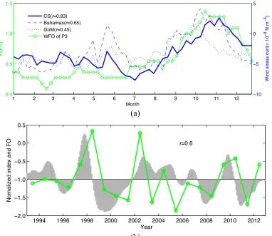
Figure 3a shows the weekly FO (WFO) of P3 along with long-term weekly mean WSC of three (Caribbean Sea (CS), Bahamas, and GoM; see Figure 1) previously identified wind influence regimes (e.g., Oey et al., 2003; Sturges et al., 2010; Gopalakrishnan et al., 2013). We found that the zero time-lag correlation coefficient between CS WSCs and WFO of P3 is 0.83, much higher than the correlations with the local WSC in the GoM (correlation coefficient r=0.45) and the downstream WSC in the Bahamas area (r=0.65). This suggests that LC eddy shedding is likely associated more with CS WSC in the upstream Caribbean Sea. Indeed, Oey et al. (2003) showed that negative CS WSC can spin up Caribbean eddies (anticyclones), which in turn lead to a lower frequency of LC shedding. Our results further reveal the CS WSC increases from June to November. It can play a role in suppressing the formation of anti-cyclonic eddies in the CS. In other words, the increase of CS WSC during this period favours a higher frequency of LC shedding, as shown in Figure 3a.

25

AFO of P3 suggests a possible connection between Pacific climate and the LC eddy shedding process.

Previous studies on the tele-connection between the Atlantic and the Pacific showed that El Niño, a Pacific event, can have a strong impact on wind and circulation in the Atlantic (Enfiled and Mayer, 1997; Alexander and Scott, 2002; Kennedy et al., 2007; Smith et al., 2007). The frequent swing in the trade winds and resulting wind stress curls in the Atlantic may favour more eddy shedding in the GoM (Chang and Oey, 2013b). Detailed processes determining how the basin-scale teleconnection influences LC eddy shedding clearly need further study that combines observations and numerical model sensitivity experiments.

5. Summary

Three patterns and corresponding temporal evolution of LC SSH were extracted from 21years of weekly satellite SSH data using the SOM method. In most cases, the LC evolution follows a normal-extension-retraction cycle. Transitions from normal pattern (P1) to extension pattern (P2) and from extension pattern (P2) to retraction pattern (P3) occur in June and the end of August, respectively.

26

nonlinearity (e.g., Lugo-Fernández, 2007), realistic dynamical modelling study is needed to better understand causes of LC shedding, vertical structure of circulation, as well as their responses to various forcing agents and climate signals.

Acknowledgement

27 References

Alexander, M., and J. Scott. 2002. “The Influence of ENSO on Air-sea Interaction in the Atlantic.” Geophysical Research Letters 29 (14): 46. doi:10.1029/2001GL014347. Chang, Y.-L., and L.-Y. Oey. 2012. “Why Does the Loop Current Tend to Shed More Eddies

in Summer and Winter?” Geophysical Research Letters 39 (5): L05605. doi:10.1029/2011GL050773.

Chang, Y.-L., and L.-Y. Oey. 2013a. “Loop Current Growth and Eddy Shedding Using Models and Observations: Numerical Process Experiments and Satellite Altimetry Data.” Journal of Physical Oceanography 43 (3): 669–689. doi:10.1175/JPO-D-12-0139.1.

Chang, Y.-L., and L.-Y. Oey. 2013b. “Coupled Response of the Trade Wind, SST Gradient, and SST in the Caribbean Sea, and the Potential Impact on Loop Current’s Interannual Variability.” Journal of Physical Oceanography 43 (7): 1325–1344. doi:10.1175/JPO-D-12-0183.1.

Cushman-Roisin, B., and J.-M. Beckers. 2011. Introduction to Geophysical Fluid Dynamics: Physical and Numerical Aspects. Academic Press.

Enfield, D. B., and D. A. Mayer. 1997. “Tropical Atlantic Sea Surface Temperature Variability and Its Relation to El Niño-Southern Oscillation.” Journal of Geophysical Research: Oceans 102 (C1): 929–945. doi:10.1029/96JC03296.

Gill, A.E., 1980. Some simple solutions for heat-induced tropical circulation, Quat.J. Roy. Metero.Soc., 106, 447-462.

Gopalakrishnan, G., B. D. Cornuelle, and I. Hoteit. 2013. “Adjoint Sensitivity Studies of Loop Current and Eddy Shedding in the Gulf of Mexico.” Journal of Geophysical Research: Oceans: 1–21. doi:10.1002/jgrc.20240.

Hurlburt, H. E., and J. D. Thompson. 1980. “A Numerical Study of Loop Current Intrusions and Eddy Shedding.” Journal of Physical Oceanography 10 (10): 1611–1651. doi:10.1175/1520-0485(1980)010<1611:ANSOLC>2.0.CO;2.

28

Kennedy, A. J., M. L. Griffin, S. L. Morey, S. R. Smith, and J. J. O’Brien. 2007. “Effects of El Niño–Southern Oscillation on Sea Level Anomalies Along the Gulf of Mexico Coast.” Journal of Geophysical Research: Oceans 112 (C5): C05047. doi:10.1029/2006JC003904.

Kohonen, T. 2001. Self-Organizing Maps. Springer.

Kousky, V. E., and R. W. Higgins, 2007. “An Alert Classification System for Monitoring and Assessing the ENSO Cycle”. Weather and Forecasting, 22, 353–371. doi: http://dx.doi.org/10.1175/WAF987.1

Leben, R. R. 2005. “Altimeter-Derived Loop Current Metrics.” In Circulation in the Gulf of Mexico: Observations and Models, ed. Wilton Sturges and Alexis Lugo-Fernandez, 181–201. American Geophysical Union.

Leben, R. R., and D. J. Honaker. 2006. “What Do We Know and What Can We Predict About the Timing of Loop Current Eddy Separation?” In ESA Special Publication, 614:19. http://adsabs.harvard.edu/abs/2006ESASP.614E..19L.

Lee, H.-C., and G. L. Mellor. 2003. “Numerical Simulation of the Gulf Stream System: The Loop Current and the Deep Circulation.” Journal of Geophysical Research: Oceans 108 (C2): 25. doi:10.1029/2001JC001074.

Le Hénaff, M., V. H. Kourafalou, Y. Morel, and A. Srinivasan. 2012. “Simulating the Dynamics and Intensification of Cyclonic Loop Current Frontal Eddies in the Gulf of Mexico.” Journal of Geophysical Research: Oceans 117 (C2): C02034. doi:10.1029/2011JC007279.

Liu, Y., and R. H. Weisberg. 2005. “Patterns of Ocean Current Variability on the West Florida Shelf Using the Self-organizing Map.” Journal of Geophysical Research: Oceans 110 (C6): C06003. doi:10.1029/2004JC002786.

Liu, Y., R.H. Weisberg, and R. He. 2006a. “Sea surface temperature patterns on the West Florida Shelf using Growing Hierarchical Self-Organizing Maps.” Journal of Atmospheric and OceanicTechnology, 23(2): 325-338.

29

Liu, Y., R.H. Weisberg, and L.K. Shay, 2007. “Current patterns on the West Florida Shelf from joint Self-Organizing Map analyses of HF radar and ADCP data.” Journal of Atmospheric and Oceanic Technology, 24(4), 702-712.

Liu, Y., R.H. Weisberg, and Y. Yuan, 2008. “Patterns of upper layer circulation variability in the South China Sea from satellite altimetry using the Self-Organizing Map.” Acta Oceanologica Sinica, 27(Supp.), 129-144.

Liu, Y., and R.H. Weisberg. 2011. “A Review of Self-Organizing Map Applications in Meteorology and Oceanography.” In Self Organizing Maps - Applications and Novel Algorithm Design, ed. Josphat Igadwa Mwasiagi. InTech.

Liu, Y., S. K. Lee, B. A. Muhling, J. T. Lamkin, and D. B. Enfield, 2012. Significant reduction of the Loop Current in the 21st century and its impact on the Gulf of Mexico. Journal of Geophysical Research: Oceans 117(C5). doi:10.1029/2011JC007555.

Lugo-Fernández, A., 2007. “Is the Loop Current a Chaotic Oscillator?” Journal of physical Oceanography 37(6): 1455–69. doi:10.1175/JPO3066.1.

Lugo-Fernández, A., and R. R. Leben. 2010. “On the Linear Relationship Between Loop Current Retreat Latitude and Eddy Separation Period.” Journal of Physical Oceanography 40 (12): 2778–2784. doi:10.1175/2010JPO4354.1.

Magaña, V., J. A. Amador, and S. Medina.1999. The midsummer drought over Mexico and Central America. Journal of Climate, 12(6).

Maul, G. A., and F. M. Vukovich, 1993. “The Relationship between Variations in the Gulf of Mexico Loop Current and Straits of Florida Volume Transport.” Journal of Physical

Oceanography 23(5): 785–96.

doi:10.1175/1520-0485(1993)023<0785:TRBVIT>2.0.CO;2.

Nürnberg, D., M. Ziegler, C. Karas, R. Tiedemann, and M. W. Schmidt, 2008. “Interacting Loop Current Variability and Mississippi River Discharge over the Past 400 Kyr.” Earth and Planetary Science Letters 272(1-2): 278–89. doi:10.1016/j.epsl.2008.04.051.

30

Oey, L.-Y., H.-C. Lee, and W. J. Schmitz. 2003. “Effects of Winds and Caribbean Eddies on the Frequency of Loop Current Eddy Shedding: A Numerical Model Study.” Journal of Geophysical Research: Oceans 108 (C10): 22. doi:10.1029/2002JC001698.

Oey, L.-Y., T. Ezer, and H.-C. Lee. 2005. “Loop Current, Rings and Related Circulation in the Gulf of Mexico: A Review of Numerical Models and Future Challenges” In Circulation in the Gulf of Mexico: Observations and Models, ed. Wilton Sturges and Alexis Lugo-Fernandez, 31–56. American Geophysical Union.

Pichevin, T., and D. Nof. 1997. “The Momentum Imbalance Paradox.” Tellus A 49 (2): 298– 319. doi:10.1034/j.1600-0870.1997.t01-1-00009.x.

Smith, S. R., J. Brolley, J. J. O’Brien, and C. A. Tartaglione. 2007. “ENSO’s Impact on Regional U.S. Hurricane Activity.” Journal of Climate 20 (7): 1404–1414. doi:10.1175/JCLI4063.1.

Solidoro, C., V. Bandelj, P. Barbieri, G. Cossarini, and S. Fonda Umani. 2007. “Understanding dynamic of biogeochemical properties in the northern Adriatic Sea by using self-organizing maps and k-means clustering.” Journal of Geophysical Research: Oceans 112, C07S90, doi:10.1029/2006JC003553.

Sturges, W., N. G. Hoffmann, and R. R. Leben. 2010. “A Trigger Mechanism for Loop Current Ring Separations.” Journal of Physical Oceanography 40 (5): 900–913. doi:10.1175/2009JPO4245.1.

Tsui, I.-F., and C.-R. Wu. 2012. “Variability Analysis of Kuroshio Intrusion Through Luzon Strait Using Growing Hierarchical Self-organizing Map.” Ocean Dynamics 62 (8): 1187–1194. doi:10.1007/s10236-012-0558-0.

Xu, F.-H., Y.-L. Chang, L.-Y. Oey, and P. Hamilton. 2013. “Loop Current Growth and Eddy Shedding Using Models and Observations: Analyses of the July 2011 Eddy-Shedding Event.” Journal of Physical Oceanography 43 (5): 1015–1027. doi:10.1175/JPO-D-12-0138.1.

Yin, X.-Q., and L.-Y. Oey. 2007. “Bred-ensemble Ocean Forecast of Loop Current and Rings.” Ocean Modelling 17 (4): 300–326. doi:10.1016/j.ocemod.2007.02.005. Yin, Y., X. Lin, Y. Li, and X. Zeng, 2014. “Seasonal variability of Kuroshio intrusion

31 Figures

32 (a)

(b)

33

34 (a)

(b)

Figure 3. (a) Weekly frequency of occurrence (WFO) for Pattern 3 (P3) and wind stress curl of the areas in Figure 1. Zero-lag correlation coefficients (r) for the relation between the WFO of P3 and the wind stress curl, at 95% confidence level for each domain, are shown in brackets after the domain. (b) Normalized Ocean Niño Index (six-month moving average; shaded area) and annual mean frequency of occurrence (FO) for P3 (green line). Correlation coefficient (r=0.6) with Ocean Niño Index lagged 90 days is shown at 95% confidence interval. 0.0 0.5 1.0 1.5 FO(%)

1 2 3 4 5 6 7 8 9 10 11 12 −10

−5 0 5

Wind stress curl(

×

10

−

8 N m

−

3)

Month CS(r=0.83)

Bahamas(r=0.65) GoM(r=0.45) WFO of P3

1994 1996 1998 2000 2002 2004 2006 2008 2010 2012

−2.0 −1.5 −1.0 −0.5 0.0 0.5 Year

Nomalized index and FO

35

Chapter III: Predictability of the Loop Current variation and eddy

shedding process in the Gulf of Mexico using an artificial neural network

approach

Xiangming Zeng, Yizhen Li, and Ruoying He

Department of Marine, Earth, and Atmospheric Sciences North Carolina State University, Raleigh, NC, USA 27695

36 Abstract

A novel approach based on an artificial neural network was used to forecast sea surface height (SSH) in the Gulf of Mexico (GoM), in order to predict Loop Current variation and its eddy shedding process. We first applied the empirical orthogonal function analysis method to decompose long-term satellite observed SSH into spatial patterns (EOFs) and time-dependent principal components (PCs). The nonlinear autoregressive network was then developed to predict major PCs of the GoM SSH in the future. The prediction of SSH in the GoM was constructed by multiplying the EOFs and predicted PCs. Model sensitivity experiments were conducted to determine the optimal number of PCs. Validations against independent satellite observations indicate our neural network-based model can reliably predict Loop Current variations and its eddy shedding process for a four week period. In some cases, an accurate forecast for five to six weeks is possible.

1. Introduction

37

north and west edges of the LC can vary from about 25.5°N to 27.5°N and 86°W to 90°W, respectively (Leben, 2005; Gopalakrishnan et al., 2013a; Zeng et al., 2015).

Daily operations of approximately 4,000 oil and gas platforms in the northern GoM are significantly affected by the LC and its high-speed eddies, which make planning and scheduling a challenge for this expensive enterprise (Leben and Honaker, 2006; Sammarco et al., 2004). Accurate prediction of the LC and LC eddies is of critical importance for both scientific research and societal benefit. For example, in order to mitigate the adverse impacts of the Deepwater Horizon oil spill in 2010, intensive research on the LC and LC eddies was performed during and after the incident (e.g., Liu et al., 2013). The LC and LC eddies also play an active role in the rapid intensification of GoM hurricanes, such as devastating Hurricanes Katrina and Rita (Leben and Honaker, 2006), which caused extensive loss of life and property damage in many Gulf coastal communities.

38

evaluated several different ocean models’ performance at LC eddy shedding prediction using various prediction skill assessment methods in the report of the GoM 3-D Operational Ocean Forecast System Pilot Prediction Project. More recently, with the four-dimensional variation method, Gopalakrishnan et al. (2013) tested the predictability of the LC eddy shedding process using the Massachusetts Institute of Technology general circulation model (MITgcm). Xu et al. (2013) applied the local ensemble transform Kalman filter with the parallel POM to estimate the states of the LC and LC eddies from April to July 2010. All these studies are based on either simple empirical relations or primitive equation ocean models focusing on a single LC eddy or a small number of LC eddy shedding events. The lack of generality makes the assessment of their model predictability very difficult (e.g., Mooers et al., 2012).

39 2. Data and method

2.1 Dataset

40

were taken from NOAA’s National Climatic Data Center and The Johns Hopkins University Applied Physics Laboratory.

2.2 Artificial neural network (ANN)

The ANN is a computational model inspired by biological neural networks that is capable of solving a variety of problems in pattern recognition, time series prediction, and parameter optimization (e.g., Jain et al., 1996). It has been widely used for variable prediction and mapping in the geoscience community (e.g., Maier and Dandy, 2000; Maier et al., 2010; Krasnopolsky, 2013). Hsieh and Tang (1998), for example, proposed the use of ANN in meteorology and oceanography, then conducted a series of applications on Pacific sea surface temperature prediction (Tang et al., 2000; Hsieh, 2001), Lorenz dynamical system forecast (Tang and Hsieh, 2001), and El Niño-Southern Oscillation analysis (Hsieh, 2004). With wind and tidal information as inputs, Lee (2006) predicted storm surge events around Taiwan Island using the ANN method. Wu et al. (2006) presented the advantage of the ANN over regression in predicting tropical Pacific sea surface temperature. Many applications also appear in pyrgeometer measurements, wind shear alerting, and climate change (e.g., Oliveira et al., 2006; Kwong et al., 2011; Yip and Yau, 2012).

41

according to the complexity of the problem. Each neuron in the hidden layer receives inputs from all the neuron outputs of the first layer. This fully interconnected procedure is repeated again in the third, output layer. The output layer has one neuron for each output variable (Oliveira et al., 2006).

Each of the three layers has its own weighting factors, which are the ANN parameters determined during the training process. The training process is the determination of the proper interconnection of weighting factors for the ANN based on training dataset patterns, so that the output of the ANN can present the best fit with the output given by the testing dataset. In this way, the ANN learns the information given in the training dataset but still has a generalizing capability, not simply memorizing the patterns in training dataset. The generalizing capabilities of the ANN guarantee that the trained model can give reasonable results for unknown patterns that differ from the training dataset (Oliveira et al., 2006). These procedures and structures give the ANN the ability of a universal approximator (Maier and Dandy, 2000; Oliveira et al., 2006).

2.3 EOF analysis

42

objective analysis of in situ data (e.g., Holbrook and Bindoff, 2000), statistical comparison between data and model results (e.g., Beckers et al., 2002), data reconstruction (e.g., Becker and Rixen, 2003; He et al., 2003; Miles and He, 2010; Zhao and He, 2012; Li and He, 2014), variability analysis (e.g., Hendricks et al., 1996), filtering (e.g., Vautard et al., 1992), and data compression (e.g., Pedder and Gomis, 1998; Rixen et al.,2002). EOF analysis can be done by applying the singular value decomposition (SVD) technique (e.g., Beckers and Rixen, 2003). Let X be a n m× matrix such that the rows indicate temporal development and the columns are variables or spatial data points. The SVD technique can break up the matrix X into three matrices:

X=U*D*VT (1) where U and V are orthonormal and D is diagonal. VT is the spatial patterns (EOFs), and U*D is the time-dependent principal components (PCs). Let λ_i be the diagonal part of D

with i=1,…,m. Then, the ratio 2 2 1

/ m

i i i

i

f λ λ

=

=

∑

is a measure of the variance contained in spatial

pattern i compared to the total variance. It is often said that PC i explains (100 f_i)% of the variance. The ratio is often the basis for deciding the number of PCs to retrain for data compression, and the ones with small ratios are usually discarded (e.g., Beckers and Rixen 2003). Usually, the ratios have been sorted in decreasing order, so that the first several PCs explain the major variance of the dataset.

2.4 Prediction Procedure

43

study leads to too large data dimension, direct SSH prediction is infeasible. To avoid the curse of dimension, EOF analysis was used to split the data into spatial EOFs and time-dependent PCs. From Eq. (1), we have

X=P*E (2) where X is our dataset, P is time-dependent PCs, and E is spatial EOFs. Eq. (2) can be written in another form:

x_1,1 ! x_1,m

" # "

x_n,1 ! x_n,m ⎛ ⎝ ⎜ ⎜ ⎜ ⎞ ⎠ ⎟ ⎟ ⎟=

p_1,1 ! p_1,m

" # "

p_n,1 ! p_n,m ⎛ ⎝ ⎜ ⎜ ⎜ ⎞ ⎠ ⎟ ⎟ ⎟

e_1,1 ! e_1,m

" # "

e_m,1 ! e_m,m ⎛ ⎝ ⎜ ⎜ ⎜ ⎞ ⎠ ⎟ ⎟

⎟ (3)

where x_{i j,} is the jth spatial SSH point at time i, n is the time index, and m is the number of spatial points.

Because the first several leading PCs represent the majority of the dataset’s variation (Table 1), we can just use the first k PCs to reconstruct the original dataset without losing much information (e.g., Beckers and Rixen, 2003). That is,

x_1,1 ! x_1,m

" # "

x_n,1 ! x_n,m

⎛ ⎝ ⎜ ⎜ ⎜ ⎞ ⎠ ⎟ ⎟ ⎟ ≈

p_1,1 ! p_1,k

" # "

p_n,1 ! p_n,k

⎛ ⎝ ⎜ ⎜ ⎜ ⎞ ⎠ ⎟ ⎟ ⎟

e_1,1 ! e_1,m

" # "

e_k,1 ! e_k,m

⎛ ⎝ ⎜ ⎜ ⎜ ⎞ ⎠ ⎟ ⎟

⎟ (4)

Similar as Alvarez et al. (2000), Rixen et al. (2001), and Alvarez (2003), we can get the approximation of SSH at time n+1 by

x_n+1,1 ! x_n+1,m

(

)

≈

(

p_n+1,1 ! p_n+1,k

)

e_1,1 ! e_1,m

" # "

e_k,1 ! e_k,m ⎛ ⎝ ⎜ ⎜ ⎜ ⎞ ⎠ ⎟ ⎟

44 if we can predict

(

pn+1,1 ! pn+1,k

)

.

The nonlinear autoregressive network with one hidden layer was chosen to do the PC prediction by following Maier and Dandy (2000). For a certain dataset, the PCs are independent of each other due to the property of EOF analysis (Hannachi, 2004). As a result, training and forecasting were applied to the PCs independently. That is,

p_{n+1, j} = f(p_{n, j},p_{n−1, j},!,p_{n−i, j}) (6) where p_{n+1, j} is the value of jth PC of GoM SSH at the

(

n+1

)

th record, and i is time delay. Because the time interval of SSH data is weekly, this prediction is one week ahead. Once we get p_{n+1, j}, we can put it into Eq. (6) and use it to predict p_{n+2, j}. The loop can continue until the accuracy decreases to the lowest acceptable level. The larger the time delay is, the longer the required training time is. Staring from i=1, we tried different time delays. Take the correlation coefficient and root mean square error (RMSE) as the performance criterion of our prediction. We found that the prediction performance improved as the increase of time delay i until i=5. Therefore, the time delay for the ANN is set to be i=5, which gives the largest correlation coefficient and least RMSE. The optimal neuron number for each PC prediction was obtained in an iterative fashion based on Kaastra and Boyd (1996)'s criteria on neuron number selection.