Article Does Sustainability Matter for Corporate Performance and Economic Development? Based on the Asia Pacific and North America

(1)

Article

Does Sustainability Matter for Corporate Performance and

Economic Development? Based on the Asia Pacific and North

America

Kyungbok Kim

1

_{, Sang-Myung Lee}

2*

_,

1 _{Department of Economics, Auburn University, Auburn, Alabama, 36849, USA; kzk0056}_@_auburn.edu 2 _{School of Business, Hanyang University, Seoul, 04763, South Korea}

*_{Correspondence: [email protected]; Tel.: +82-2-2220-2594}

Abstract:

This paper explores how the sustainable investment impacts financial returns and economic development in of Asia Pacific and North America, utilizing real data empirically. In academia and industrial field, it is polemical that indeed, the sustainable behavior has economic returns. In order to clarify that, we tested hypotheses with an analysis of seven stock markets, accounting of rates such as ROI, ROIC, and ROA in eleven companies, and GDP/GNI per capita. The results indicate that both financial return and economic development are positively germane to the sustainable investment. Besides, the variance of sustainability to economic development exists, depending on GDP per capita between two regions. We conclude, concerning the sustainability, by corroborating micro perspective for corporate level and macro perspective of economic development in the private and public sector. This research consequence will be interested in both practitioners and researchers in the measurement

of sustainability performance.

Keywords: sustainable investment, corporate performance, economic development, VAR, and VECM

1. Introduction

(2)

Being following that everything is changing because of the climate change including technological development, everyone knows and recognizes that industrial revolution has destroyed the environment, even though our lives have been comfortable. UNEP FI [79] report says that the activities of the world’s 3,000 biggest companies estimate on third of profits would be lost if firms were forced to pay for use, loss, and damage to the environment as well as world’s top firms cause $2.15 trillion of environmental damage. As mentioned above, if many companies do not protect the environmental issues in which climate change, water scarcity, food security and deforestation have emerged, they are not able to obtain sustainable competitive advantages such as getting various scenarios for future. The corporate sustainability is becoming significant as mainstream for now and future’s growth engine. In the theoretical and empirical research papers, it demonstrated that why companies do need the sustainable strategy because there was positive relationship between sustainable management and financial returns as evidence by [16,39,48,49,75].

Previously on literature review, measuring sustainability was like a conundrum because it has two characteristics. Firstly, the sustainability has a long term figure [16]. Measuring performance about sustainable activities needs many times with the precise data. It means previous works have not been timely and infelicitous. Sustainable performance is analogous to build up for enterprise strategies, forecasting multiple scenarios in the long-term period. For here, it is opaque that long-term cannot be calculated precisely. In the stock market, similarly, there is a calculation method for sustainable growth rates of companies using accounting of rates such as financial statements. Through various measuring tools like financial or predictive modeling based on demand forecast, we can figure it out. To differentiate the former works, this research analyzes the financial data and stock price of companies in comparison with sustainability index by time series method. Secondly, according to European Commission’s report [22], it is murky that almost all sustainable assessment studies end up comparing different alternative scenarios with the evaluation trying to individuate which alternative way leads to a more sustainable development. It is very obscure to evaluate how much certain products, policy or institution can contribute to its fulfillment. Therefore, this paper shows empirical evidence, surmounting two characteristics as noted above. In order to do that, we explore the empirical data from a historical and authentic institution with industry issues. Plus, we reckon the analyses on as-is and future of the sustainability are crucial to overcoming its uncertainty by portraying prediction model.

(3)

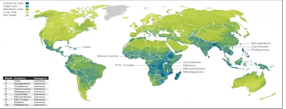
Sources: KPMG US(2012) and Maplecroft(2012), The Climate Change and Environmental Risk Atlas. Available at http://maplecroft.com - Restructured

Figure 1 indicates vulnerability of climate change throughout the world. As elucidated about climate change, it is the global mega forces that impact all others such as water scarcity, energy and fuel, deforestation and ecosystem decline directly. Our paper focuses on North America and Asia Pacific region. There are two reasons why we picked. The first one is a deficiency of data for Africa where climate change is highly susceptible. The second one is that Asia Pacific is the second vulnerable region in climate change of sustainability. So this region will be compared by well-performed region such North America.

Our salient research question is how well companies operate sustainable management by climate change and why companies need the competitive advantage from it. Here we examine the empirical analysis that the relationship between investment in sustainability and economic and financial is inevitable regarding utilizing stock indices and DJSI, which is based on an analysis of corporate economic, environmental and social performance, assessing issues such as corporate governance, risk management, climate change mitigation, supply chain standards and labor practices by utilizing theories of investment, and development economics. The contribution of this paper is why many companies need the sustainable management like managerial implications by analyzing empirical data. We also show academic implications that the firm’s capacity, having the sustainability and corporate performance, has the competitive advantages against no evidence between economic returns and sustainability.

2. A theoretical framework for the hypothesis

2.1. Definitions of Sustainability in previous literatures

With respect to the sustainability, people tend to think that sustainable management is an environmentalism. It, however, is the wrong assumption. Traditionally, it is not only the managerial influence on balance including economic, environmental and social issues but also the management technique with financial and non-financial performance such as total sales, net profit, and ethnic, environmental and social problems. That is what people call corporate social responsibility, ethnic or stakeholder management. In the former works about sustainable management, it has been denoted as eclectic definitions. For example, Dyllick and Hockerts [19] have declined corporate sustainability as: “meeting the needs of the firm’s direct and indirect stakeholders(such as shareholders, employees, clients, pressure groups, communities, etc.,.) without compromising its ability to meet future stakeholders needs as well”. Marrwijk [45] explained that corporate sustainability refers to “demonstrating the inclusion of social and environmental concerns in business operations and interactions with stakeholders”. Like many others, these definitions build on stakeholder theory, which is one of the most widely applied theoretical frameworks for research on corporate sustainability written by [60].

(4)

sustainability is based upon efﬁciency in the transformation process and equity in the distributive effects. The World Commission on Environment and Development have manifested the sustainability as the ability to “meet the needs of the present without compromising the ability of future generations to respond to their needs.” In fact, being sustainable is now becoming a source of competitive advantage and a matter of corporate survival rather than a costly inconvenience. A process of sustainability facilitates to create a vibrant economy and a better quality of life while respecting the need to sustain natural resources and protect the environment. It can express as the principle that future generations should live in a world that the present generation has enjoyed but not diminished. To sum up, most of proposed definitions state that corporate sustainability subsumes the variety of aspects that need to be considered simultaneously and is often clustered into three main sub-groups; Environmental (E), Social (S), and Governance (G), like systematic concept, associating with the continuity of economic, social, institutional and environmental perspectives of human society [79]. Hence, in this paper, we define as the ESG that is a catch-all term for measuring corporate sustainability.

2.2. The Sustainability and Corporate Performance on Investment Theory

It is controversial that the relationship between financial or economic returns and sustainable behavior is positive or negative. There are several kinds of literature having no correlation between them. Margolis and Walsh [42], found no evidence that embracing sustainability increases profitability. The work of Palmer and Siebert suggested that as the environment and natural resources are the main production factors, imposing limitations on them will increase costs and limit the firm’s ability to grow written by [69,74]. Hansen et al. [30] indicated that the relationship between a comprehensive set of social and environmental indicators and financial performance over the previous two years for 1,100 CEOs had no correlation between them. Neoclassical economists often base their arguments on the shareholder theory, stating that the only social responsibility of business is to increase profits and that doing otherwise, such as investing resources in costly sustainability initiatives, will necessarily reduce shareholder value by Friedman [23].

The most important thing is that people who are making the policies recognize sustainable management like environmentally utilizing resources is the nugatory investment since they think it is only for future, not in the present as well as not physical consequences immediately. There is the evidence that the Boston Consulting Group [10] had surveyed to 1,500 corporate executives and managers from companies individually throughout the world. It came up with the results that more than 70 percent of survey respondents showed their company had not developed a clear business case for sustainability and self-identified experts in sustainability believed more strongly in the importance of engaging with suppliers across the value chain. In addition to that, sixty-two percent of these respondents considered it necessary to hold providers to specific sustainability criteria. Of course, only this research does not mean why the sustainable management is significant in whole industries.

(5)

investing influences on stock returns by lowering the book to market ratio and not by generating positive alphas. Research on corporate sustainability has shown deference to business orthodoxy as scholars strive to prove the business case for sustainability, and in doing so fit it into the dominant beliefs embedded within business literature by [2,32,46,59].

Fundamentally, we reckon that corporate performance comes from many and various factors. Among them, the overarching cause can be as the investments for accretion of firms through institutional investors. According to U.S. Securities and Exchange Commission, the growth in the proportion of assets managed by institutional investors has been accompanied by a dramatic increase in the market capitalization of U.S. listed companies. For example, in 1950, the combined market value of all stocks listed on the New York Stock Exchange (NYSE) was about $94 billion. By 2012, however, the domestic market capitalization of the NYSE was more than $14 trillion, an increase of nearly 1,500 %. This growth is even more impressive if you add the $4.5 trillion in market capitalization on the NASDAQ market, which did not exist until 1971. As mentioned for institutional investors above, why do they invest a lot of money to company’s stock? The answer to a question is indubitable that they want to get money back as much as they invested and to obtain savings. Plus, in another aspect, many companies need the investments from them as well due to a reason why in general, the business expansion for the future accrues the competitive advantages of their own eventually. In the investment theory, there are two motivations for the investment. Goetzmann [27] addressed that motivation of the investment is the desire to increase wealth (i.e. make money grow). Another one is the desire to pass money from the present into the future. People and organizations anticipate future cash needs and expect that their earnings in the future will not meet those needs.

In order to prove the relation between sustainability investments and financial performance, we utilize ROI(Return On Investment), ROIC(Return On Invested Capital), and ROA(Return On Asset). These financial statements are the overarching factors to evaluate company’s financial performance measures and investment returns. There is evidence that firms have begun to monitor and track some of these measures through internal cost-benefit analyses and activity-based costing [47,66]. Basically, ROI shows how companies invest efficiently, and the value of ROIC subsumes not only the firm earns the cost of capital but also how much they invest. ROA denotes how efficiently firm yields the income using its assets. We reckon that the firms, are with accounting rates of return such as ROA, ROI, and ROIC, have better performance than the firms that are not doing sustainability. In the previous work of accounting rates and sustainability, Robert et al. [56] corroborated that the performance between high sustainability companies and low sustainability companies was different in long-term by comparing samples of 180 US firms. The results showed that high sustainability companies were significantly outperformed over the long-term, using variables such as ROE, ROA, stakeholder engagement, the disclosure of nonfinancial information, and governance. In this work we concentrate on ROI, ROIC, and ROA, differentiating former works because they are reasonable when evaluating revenues based on an amount invested not a sales account. This point can reduce the distortion that an index like total sales has extensive benefit rates including ROA, ROE. In other words, if we use the ROIC in a company, we will see purely benefit rates based on how much we invest.

(6)

research for the relation between financial returns and the sustainability has been corroborated positively although there was an argument in which several types of research showed no evidence and findings. What we are going to underline is to find their causality, but not a correlation between them. Corporate investment in the sustainability is to determine valuable values for the future’s competitive advantages as well as by augmenting the present value of a company such as economic benefits; financial performance will be increased. Accordingly, we hypothesize the positive causality between stock investment and sustainability:

Hypothesis 1: The causality between the sustainability and financial returns will be positively associated with firm’s present and future values.

Hypothesis 1-1: Major capital flows of a stock market in both North America and Asia Pacific area will have a positive relationship with sustainable investment.

Hypothesis 1-2: Firm’s stock prices, which are on sustainable management in both North America and Asia Pacific area will be positively associated with the sustainable investment.

Hypothesis 1-3: Firm’s accounting of rates with ROI, ROIC, and ROA will be positively associated with sustainability investments.

2.3. Regional Differences of Sustainability Performance on Economic Development Theory

The prominent norm of the sustainability performance among countries depends on two situations at which we focused on our paper, even though there are many standards to appraise the sustainability performance. The first one is how much the money has been invested in the industries of its country. Another one is how well the countries have been burgeoned economically, purporting that ESG (Environment, Social, and Governance) is embraced. Asia is not only to be faced with the environmental problems of air pollution, water management, and land degradation but also to have wicked problems meaning there are many brittle nature circumstances. In the last decades, East Asia-Pacific such as China has been burgeoned even though there have been precarious situations economically. Coxhead [14] verified the analysis on the features of the relationship between economic growth and environmental resources in different parts of the region. Zhang [77] contemplated environmental degradation due to burgeoning energy demand across Asia and recommended several policies to address the increasing prominence of this issue as economic expansion continues. There is the other research concerning the relevance of the regional economy and environmental issues.

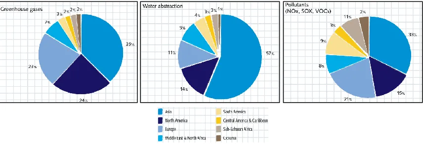
Bawa et al. [7] explored the competitive use of resources by India and the PRC, the need for inter-state cooperation over environmental issues, and the impact of these major players in the broader region. In figure 2, what they have in common is that the each rate of greenhouse gases, water abstraction, and pollutants in Asia takes possession that is the most substantial proportion in these charts. Especially East-Asia has been in high economic growth rate throughout the world from 2006 to now as well as a lot of environmental capital is flowing in. There is evidence that in 2014 notably, buyout-backed exists in Asia-Pacific markets shot up to nearly $53 billion, a 120% increase by [6].

(7)

greenhouse gas, water abstraction, and pollutants, both Asia and North America have huge proportion. Why do two regions have environmentally maladies? Estimating differences in economic growth rates, population, and GDP indicates that how well each nation experiences the economic development. This paper concentrates on the role of sustainability, generating that regional disparity exists in economic development.

What is the development? There are a lot of definition about it, but we make it simple using Sumner and Tribe’s [72] words. They defined as three categories; 1) short to medium term outcome of attractive targets, 2) long-term process of structural societal transformation, 3) a dominant discourse of western modernity. The development we referred to the literature review above looks analogous with the sustainability as we discussed in the previous section. Yes, this point we assume is the final goal for our research which means the sustainability has the tremendous importance of economic development. To do that, we need to look for its attributes like what factors are germane to causality between them. Albeit there is a difference depending on the subject of pioneering researchers such as Smith, Marx, Schumpeter, Lewis, and Rostow in many former types of research for the economic development, we found the properties approaching the theory of economic development in Table 1. Our research, however, underscores whole theories regardless of that each time in development economics has leading models. What it means that even if we utilize the prevailing theory in advanced sequences, new growth theories have been failed with the method of coordination such as government intervention and underdevelopment.

Figure 2. Regional Rate of Environmental Issues

(8)

Table1. The evolution of development economics

By time Main Key Words and Models(Theories) Researchers

Early Views

▪ Capitalism; free trade, private property and competition Smith [71] ▪ Communism; social or public ownership of property, and

independence of foreign capital and goods Marx [43] ▪ Technology; business cycles, innovation, socialism Schumpeter [70]

Classical Theories

▪ Linear Stage Growth Model Rostow [58], Harrod [29], Domar [18]

▪ Structural Change Model Lewis [50], Chenery [12]

▪ International Dependence Model Singer [65], Baran [9] ▪ Neoclassical Counter Revolution Model Stiglitz [68]

Contemporary Theories

▪ New Growth Model; knowledge, role of public sector

and investment Aghion [3], Sen [63]

The goal of economic development in its simplest form is to improve the quality of life and to be sustainable development as well as the most significant thing is to bring about the growth such as gross income per capita. Before the 1970s, rapid economic growth has been considered a good proxy for other attributes of development [76]. There are many ways to evaluate the economic development. In our paper, we concentrate on GNP and GDP which have properties to elucidate the importance of sustainability and economic development empirically. Giang and Sui [25] demonstrated that financial performance is measured by an annual increase in gross national product (GNP) and World Bank estimates it as GNI per capita. Also, Caroll and Stanfiled [11] utilized the factor like stock price and GDP substantiating that regional development design generates sustainable economic development. In comparison with previous research, there was no multi-faceted sustainability performance regionally and empirically while what we distinguish is by two instructions using both stock prices into local investment and GNP/GDP. In summary, regional difference and the link between sustainability and economic development leads directly to our second hypothesis:

Hypothesis 2: The sustainability will exist the regional differences of economic development between Asia-Pacific and North America.

Hypothesis 2-1: The gross national income (GNI) and gross domestic product (GDP) that are overarching factors for economic development will be positively associated with sustainability investment in each region.

(9)

3. METHODS

VAR Properties. Our goal is to figure out for the causality among the sustainability performance, financial returns, and economic development. To do this, we require using VAR (Vector Autoregressive), model. In the former researches, it has been utilized for analyses such as financial data, stock prices/returns, and money supply by [40,51,52,]. The VAR model in economics has made popular by Sims [64]. Especially it is proven to be useful for describing the dynamic behaviors of economics and financial time series and for forecasting as well as it has been known as the model from univariate autoregressive to multivariate autoregressive frequently using for projection and efficiency analysis by the change of endogenous variables. Zivot and Wang [78] indicated that the VAR model is used for structural inference and policy analysis. In structural analysis, certain assumptions about the causal structure of the data under investigation are imposed, and the resulting causal impacts of unexpected shocks or innovations to speciﬁed variables on the variables in the model are summarized. Utilizing VAR model that a change of any one variable can be determined by an endogenous variable in the dynamic response, our goal concentrates on the causality, not a correlation between investing sustainability and financial returns.

Table 2. How to operate time series model

Div. Univariate Multivariate

Stationary ARMA Model VAR Model

(Vector Autoregressive)

Non-Stationary Unit Root Test VECM

(Vector Error Correction Model)

There is a difference about between time-series and cross-sectional data. Based on the stationarity of variable, time series analysis satisfies its assumption and has the efficiency. When their variables have non-stationarity, they have to be eradicated for detrending before estimating a specific VAR model. The first thing we do is to employ the Augmented Dickey-Fuller (ADF) and Phillips-Person (PP) unit root tests for the multivariate approach of Johansen and Juselius [35]. After ADF test, if the variable is non-stationary, we have to treat the first difference of variable indicating that non-stationary variable modifies into being stationary. Then, given nature of results, we can make a decision selecting the lag length. As denoted in Table 2, our paper is embraced in ‘multivariate’ analyzing our hypotheses by VAR and VECM. Why we choose this VAR model is that first, it is lucid the impulse response analysis attests a change of one variable in endogenous variable influencing dynamic effects. Secondly, through the variance decomposition, we can analyze the size of the contribution of these variables to the total variation in each endogenous variation. What it means is that VAR does not settle on the hypothesis by economic theory but analyzes real economy using given economic time series. In other words, it makes systematic outputs utilizing parallax variable like an explanatory variable to all variables.

(10)

Part Region Independent Variables

Hypothesis 1

Asia Pacific

▪ Nikkei 225 (NK) ▪ KOSPI (KP) ▪ Hong Kong Hangsen (HKH)

▪ Shanghai Shenzhen (SS) ▪ AUS 200 (AUS)

North America ▪ NASDAQ (ND) ▪ S&P 500 Total Revenue (SP) Asia Pacific

(Each company’s Stock Price, ROI, ROE,

and ROIC)

▪ Samsung Electronics (SE) ▪ Seven and Holdings (SH) ▪ Toyota Motors (TM)

▪ NTT Docomo (NTD) ▪ West Banking (WB) ▪ Astellas Pharma (AP)

North America (Each company’s Stock Price, ROI, ROE,

and ROIC)

▪ Apple Inc. (AI)

▪ Exxon Mobil (EM) ▪ Johnson and Johnson (JJ)

▪ Pepsi Co. Inc. (PCI) ▪ Verizon (VZ)

Hypothesis 2

Asia Pacific and North America

▪ Gross National Income per capita ▪ Gross Domestic Product per capita

Dummy Variables

▪ Great Recession (2008 and 2009) ▪ Population by each region

* Sources: World Bank, APEC, Federal Reserve Bank of St. Louis, Each company’s stock by searching * Period: Hypothesis 1 (2010-01-04 through 2015-12-07),

Hypothesis 2 (1998-01-04 through 2016 of GDP (Quarterly) and GNI (Quarterly/Annually) by each region) * Dependent Variables: Dow Jones Sustainability Index by each region

Modeling and Data. In order to clarify the relationship between sustainability performance, financial returns, and economic development, we have garnered the variables such as the data of stock market regionally, each firm’s stock price, macro economy factors. Many types of research have demonstrated the relation among stock market, stock returns, and specific economic variables by [5,17,31,38,41,73]. This paper has difference contributions in comparison with them. First, it extends regional stock markets in Asia-Pacific and North America including a particular topic, the sustainability performance empirically. The only conceptual ‘buildup’ was operated a lot because it is demanding to gather real data as well as the hardship exists to measure quantitatively. Hence, we settle on a variable of sustainability performance by DJSI (Dow Jones Sustainability Index) which is factual data. Its conceptual definition is analogous to what we define in Section 2.1.

(11)

respectively. These are all responsible for handling and organizing the investment in each region; 2) constituting stock prices of top 5 sustainability companies of DJSI regionally; 3) using the variables of accounting of rates such as ROI, ROIC, and ROA from a financial corporation, ‘Five Tree.' Hypothesis 2 portrays the causality between sustainability performance and economic development by GDP per capita and GNI per capita. To avert the multicollinearity, it requires other variables because depending on the population, especially the values of GDP and GNI can be a discrepancy in which two predictors in multiple regression models are highly correlated indicating that one variable may be linearly predicted from the others with an equivalent degree of accuracy. We focus on GNI and GDP as mentioned in theory building of the last section, albeit macro economy has many indicators like money supply, CPI, and un/employment. The time setting for hypothesis 2 is from 1998 to 2016 because economic development is not ‘fleeting innovation,' while hypothesis 1 which is germane to the sustainability settles on 2010 through 2016. Plus, all variables were modified to logarithms to set up the normal distribution at which regression equation is stable.

When the time series variables have stationarity, the first model of time series we can consider is the ARIMA. However, that has the limited option in which they utilize only the information related to their past. In order generally to observe the relationship between each variable, ARIMA model has some limitations that do not consider with additional information such as factors. Therefore, we need to add the other variables influencing on the dependent variable. By adding vectors , AR model treats scalar variable, while VAR model deals with a vector which means dependent and explanatory variable. Hypothesis 1 construes the causality between sustainability performance and economic value, especially financial returns. To do so, we use the VAR basic model in (1) as below,

t p t p t t

t

y

e

Y





1 1 



2 2 ....



  ,

e

t~i.i.d. (0, Ω) (1)

Only,

Y

t [

t

Y

₁_,

t

Y

₂_, ],



1= [

11



12

21



22

],

e

t= [ t

e

₁

t

e

2 ]

For here,

Y

t (

Y

1t...

Y

2t...

Y

kt) constitutes the vector, some “k” endogenous variable of analysis

target. If we use VAR model, it is possible to consider how other variables affect our objective

variable,

Y

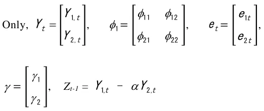
t. All time series variables should accord with stationarity so then they forestall the

significance of endogenous variables to diverge. If our variables have unsated stationary time series, we modify to VECM (Vector Error Correction Model), in (1) following that to estimate

co-integration relationship, the stationarity satisfies to add lagged variables, Zt-1.

t p t p t t t

t

z

y

e

(12)

Only,

Y

t [ t

Y

₁_,

t

Y

₂_, ],



1= [

11



12

21



22

],

e

t= [ t

e

₁

t

e

₂ ],



= [



1 2



], Zt-1 =

Y

1,t -



Y

2,t

It is possible that VAR analysis can be applied for dummy variables [54]. We define the dummy variable as zero and one (0, 1). When the GNI and GDP have the over value compared to an average value in each time, the value is one, 1. Otherwise, zero, 0. As mentioned in Figure 4, we set another dummy variable such as GR (Great Recession) from 2008 to 2009 as their variables need to get the shock mitigation not influencing on the other variables.

Preliminary Analysis: ADF and KPSS Test. In order to verify the stationarity of VAR model, we employ the ADF and KPSS analysis of unit root test individually. The estimation of ADF test is

in (3), and a null hypothesis is H0 :



=0. We assume that if a null hypothesis cannot reject, the unit

root exists.

t K

j

j t j t

t

y

e

Y

   





 

 1 1 2

1









(3)

Showing the consequences of ADF and KPSS test in Figure 6, we reject a null hypothesis meaning that unit root exists. However, after first difference in KPSS test, all variables have the stationarity. In this regard, Eagle and Granger [21] substantiated that even if there is the change of trend in individual economic time series to abnormal set (or unstable) and if the linear combination having stationary time series in the long term exists, the linear combination becomes stationary time series variable. In other words, these time series variables are in a co -integrating relationship. However, it has the deficiency when the co-integrating vector is two more or over. So Johansen [36] found that when variables are non-stationary, it is possible to modify the alternatives such as vector error correction model (VECM) after performing the co-integration test. As we settle on not only a standard of time series analysis in Figure 4, but also literature review as mentioned above, the remainder of variables is operated by vector error correction model (VECM) except for log(ND), log(NTD), and log(AP_GDP). To lay the groundwork for VECM, we operate the co-integration test such as Johansen test before (See Appendix).

(13)

Variables

(Log values) Lag

ADF Test (Asymptotic p-value)

KPSS Test (After first difference)

DJSI_APTR 3 0.2663 0.0494***

SP 6 0.3586 0.0432***

DJSI_NATR 6 0.1252 0.0350***

ND 6 0.0966* 0.0338***

AUS 9 0.5919 0.0838***

HKH 3 0.1626 0.0311***

NK 5 0.3870 0.1812***

SS 5 0.7615 0.1820***

KP 8 0.1152 0.0678***

AI 3 0.6133 0.1854***

AI ROA 2 0.7854 0.11451**

AI ROI 2 0.7706 0.11873**

AI ROIC 2 0.9916 0.1919

JJ 3 0.5118 0.1097***

JJ ROA 2 0.5263 0.1013**

JJ ROI 2 0.474 0.09113*

JJ ROIC 2 0.1413 0.1890***

EM 6 0.8878 0.1602***

EM ROA 2 0.9938 0.3328

EM ROI 2 0.9945 0.3225

EM ROIC 2 0.9454 0.2564***

PCI 6 0.2567 0.0381***

PCI ROA 2 0.6134 0.18212***

PCI ROI 2 0.947 0.25858***

PCI ROIC 2 0.7627 0.0936***

VZ 3 0.8888 0.1000***

VZ ROA 2 0.7322 0.138304***

VZ ROI 2 0.9056 0.1712***

VZ ROIC 2 0.8623 0.13447***

SE 3 0.7589 0.1226***

SE ROA 2 0.02** 0.08427*

SE ROI 2 0.1636 0.0761*

SE ROIC 2 0.639 0.10265

TM 3 0.9647 0.3699*

TM ROA 2 0.789 0.090*

TM ROI 2 0.6846 0.0941

TM ROIC 2 0.7539 0.09741*

NTD 2 0.1000* 0.2121***

NTD ROA 2 0.04274** 0.0861*

NTD ROI 2 0.03814** 0.0875*

NTD ROIC 2 0.1558 0.07932*

AP 3 0.1404 0.1549***

AP ROA 2 0.3804 0.08343

AP ROI 2 0.3528 0.0713*

AP ROIC 2 0.669 0.103959

SH 3 0.9455 0.1719***

SH ROA 2 0.2475 0.06941*

SH ROI 2 0.3069 0.0845*

SH ROIC 2 0.543 0.06347*

WB 6 0.7358 0.0794***

WB ROA 2 0.06568* 0.0970*

(14)

※ KPSS Test: Critical Values: *p < 10%, **p < 5%, and ***p < 1%, depending on how much variables have the samples

4. Results

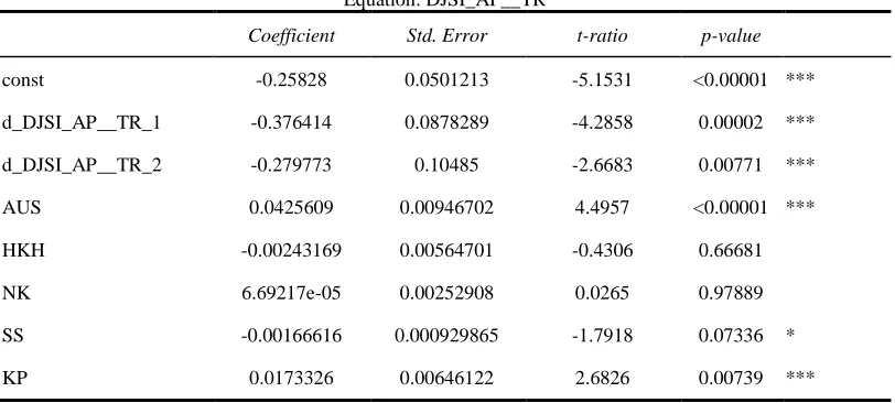
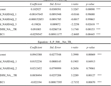
According to the result of hypothesis 1-1, using VECM in daily data from 2010 to 2015, the sustainability performance in Asia Pacific is positively associated with Asia major stock markets such as AUS (<0.00001), SS (0.07), KP (0.007) in Table 5. The rest, NK, and HKH, however, are not significant with sustainability total returns. A determinant of variable stationarity, eigenvectors are 0.05, 0.03, 0.02, 0.01, 0.008, and 0.005 indicating that they are stationary, le ss than one, ‘1’(See the Appendix). In North America, the consequences of VECM show that ND and SP have highly strong relation with sustainability performance. Albeit many companies are registered in ND and SP respectively, they are pertinent to the investment and financial returns like economic values. That is a crucial reason why this research determines vector autoregressive analysis instead of correlation between them. Their eigenvectors are stationary. In other words, this VECM is stable.

Table 5. Results of Hypothesis 1-1 in Asia Pacific

Equation: DJSI_AP__TR

Coefficient Std. Error t-ratio p-value

const -0.25828 0.0501213 -5.1531 <0.00001 *** d_DJSI_AP__TR_1 -0.376414 0.0878289 -4.2858 0.00002 *** d_DJSI_AP__TR_2 -0.279773 0.10485 -2.6683 0.00771 *** AUS 0.0425609 0.00946702 4.4957 <0.00001 *** HKH -0.00243169 0.00564701 -0.4306 0.66681 NK 6.69217e-05 0.00252908 0.0265 0.97889 SS -0.00166616 0.000929865 -1.7918 0.07336 * KP 0.0173326 0.00646122 2.6826 0.00739 ***

*p < 10%, **p < 5%, and ***p < 1%

WB ROIC 1 0.443 0.07282*

AP_GDP 7 0.0044*** 0.0451***

AP_GNI 1 N/A 0.3200***

NA_GDP 3 0.3293 0.3134*

(15)

Table 6. Results of Hypothesis 1-1 in North America

Equation : NASDAQ

const 0.102927 0.0309391 3.3267 0.00090 *** d_NASDAQ_1 -0.00147645 0.0891948 -0.0166 0.98680 d_NASDAQ_2 -0.000152853 0.0891785 -0.0017 0.99863 d_NASDAQ_3 -0.19826 0.089072 -2.2258 0.02618 ** DJSI_NA__TR 0.091003 0.0286718 3.1740 0.00153 *** EC1 -0.0259547 0.00911177 -2.8485 0.00445 ***

Equation : S_P_500__Net_TR_

const 0.0943388 0.0277548 3.3990 0.00069 ***

d_NASDAQ_1 0.0152236 0.0800145 0.1903 0.84913

d_NASDAQ_2 0.0212452 0.0799999 0.2656 0.79061

DJSI_NA__TR 0.0830494 0.0257208 3.2289 0.00127 ***

EC1 -0.022194 0.00817395 -2.7152 0.00670 ***

*p < 10%, **p < 5%, and ***p < 1%

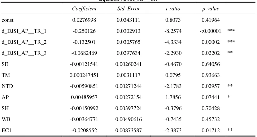
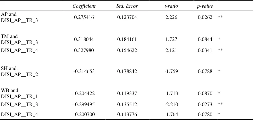
In order to verify the relation between sustainability performance and financial returns, we estimate the causality with specific variables for hypothesis 1 -2. Table 7 and 8 present that the most of top 5 companies, which have the efflorescence on sustainability in each region, are germane to financial returns. Of course, statistically several companies such as SE, TM, SH, and WB in Asia Pacific, also for AI, JJ, and VZ in North America, are not significant but as seen in Table 9, AP, TM, SH, and WB are all significant with sustainability total returns after individual VECM analysis by putting them to endogenous variables. That is because, in one of the properties in VAR, it is not necessary to worry which variable is the endogenous variable and which is the exogenous variable [37]. The remainders of independent variables, AI, JJ, and VZ do not have the significance against sustainability total returns after even analyzing individual VECM. For here, there is an implication that we need to categorize by industry and then to figure out for why these companies have the significance through an in-depth case study.

(16)

between the efficiency of investment and sustainable management. It assumes carefully that high sustainable management will be outperformed in comparison with not doing sustainable management. We accentuate that sustainable management encompasses all of the corporate processes. To preser ve the environment, the firms have not only to develop technologies using their core competencies but also to take the contribution to society; they try to solve the poverty as volunteers, donating one part of their revenues. Plus, by taking organizational governance, the firms let investors know that a company uses accurate and transparent accounting methodologies, and also they help them to see that common stockholders are allowed to vote on significant issues.

Equation : DJSI_AP__TR

const 0.0276998 0.0343111 0.8073 0.41964 d_DJSI_AP__TR_1 -0.250126 0.0302913 -8.2574 <0.00001 *** d_DJSI_AP__TR_2 -0.132501 0.0305765 -4.3334 0.00002 *** d_DJSI_AP__TR_3 -0.0682469 0.0297634 -2.2930 0.02202 ** SE -0.00121541 0.00260241 -0.4670 0.64056 TM 0.000247451 0.0031117 0.0795 0.93663 NTD -0.00590851 0.00271244 -2.1783 0.02957 ** AP 0.00485957 0.00272154 1.7856 0.07441 * SH -0.00150992 0.00397724 -0.3796 0.70428 WB -0.00364771 0.00490616 -0.7435 0.45732 EC1 -0.0208552 0.00873587 -2.3873 0.01712 **

*p < 10%, **p < 5%, and ***p < 1%

Table 8. VECM Results of Hypothesis 1-2 in North America

Equation: DJSI_NA__TR

(17)

d_DJSI_NA__TR_5 -0.23167 0.0740189 -3.1299 0.00178 *** AI -0.00078442 0.000748456 -1.0481 0.29479 JJ 0.00493479 0.00543489 0.9080 0.36403 EM 0.0136437 0.00481917 2.8311 0.00470 *** PCI 0.0149709 0.00827384 1.8094 0.07059 * VZ -0.00567402 0.00517378 -1.0967 0.27296 EC1 -0.102535 0.0184821 -5.5478 <0.00001 ***

*p < 10%, **p < 5%, and ***p < 1%

AP and

DJSI_AP__TR_3 0.275416 0.123704 2.226 0.0262 **

TM and

DJSI_AP__TR_3 0.318044 0.184161 1.727 0.0844 * DJSI_AP__TR_4 0.327980 0.154622 2.121 0.0341 **

SH and

DJSI_AP__TR_2 -0.314653 0.178842 -1.759 0.0788 *

WB and

DJSI_AP__TR_1 -0.204422 0.119337 -1.713 0.0870 * DJSI_AP__TR_3 -0.299495 0.135512 -2.210 0.0273 ** DJSI_AP__TR_4 -0.200700 0.113776 -1.764 0.0780 *

*p < 10%, **p < 5%, and ***p < 1%

Table 10. Results of Hypothesis 1-3 in North America and Asia Pacific

Accounting of Rates Adjusted R-squared F-value Sum squared

resid p-value(F)

North America

ROI 0.436652 2.660931 0.421648 0.09 * ROIC 0.400598 2.432132 0.448633 0.1 * ROA 0.477294 2.956687 0.391229 0.07 *

Asia Pacific

ROI 0.832195 10.29866 0.065429 0.002 *** ROIC 0.764873 7.099418 0.091679 0.008 *** ROA 0.843936 11.13932 0.060851 0.002 ***

(18)

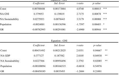
As a long literature has suggested for the relation between macro-economy variables and economic growth, our paper has the characteristics analyzing real and authentic data of sustainability, firm’s accounting of rates, and macro- economy variable like GDP per capita and GNI per capita. As a result, Table 11 shows that it is manifest that GDP(0.05915) and GNI (0.03319) are significant with the sustainability total returns in Asia Pacific as well as eigenvalues are stationary, less than ‘1’(See Appendix). North America’s consequences of GDP and GNI against the sustainability are 0.00088 and 0.0285 respectively.

To test hypothesis 2-2, we use forecast error variance decomposition. The difference between regions exists precisely. Asia Pacific, for example, has the proportion that after the 15th quarters, sustainability variance explains 65.59%. Meanwhile, GDP and the population of variance contri bute to sustainability with 9.86% and 24.55% respectively while in North America, sustainability variance expounds on 51.03% and the rest variances account for GDP 24.68% and population 2.56%. Table 13 denotes these results. Depending on that the quarters, we know how the values of indicators like sustainability and GDP can be predicted. The findings for hypothesis 2 -2, then provide, not vague explanations, support for an idea that why the sustainability in Asia Pacific area has the importance for future because it would be the overarching factor for near future. In summary, the results are consistent with the hypotheses developed above. We know the ramification that how the impact of the sustainability to financial returns and economic development influence s on several industries.

Table 11. Results of Hypothesis 2-1, GDP and GNI per capita in Asia Pacific

VECM

const 0.106917 0.133464 0.8011 0.42680

Population_log__1 0.054724 0.0266501 2.0534 0.04518 ** Population_log__2 0.0501459 0.0266954 1.8784 0.06604 *

AP_Sustainability_7 -0.226886 0.132538 -1.7119 0.09300 * AP_GDP_ 0.034562 0.017906 1.9302 0.05915 *

EC1 -0.0334078 0.0264163 -1.2647 0.21174

*p < 10%, **p < 5%, and ***p < 1%

ARIMA

Coefficient Std. Error z p-value

Const 18.5077 5.19202 3.5646 0.00036 *** phi_1 -0.11305 0.251165 -0.4501 0.65264 theta_1 1 0.309313 3.2330 0.00123 *** AP_Sustainability 2.29636 1.07819 2.1298 0.03319 **

(19)

Table 12. Results of Hypothesis 2-1, GDP and GNI per capita in North America

Equation : GDP

Const 0.00708408 0.00173884 4.0740 0.00015 *** NA GNI 0.379953 0.139819 2.7175 0.00878 *** NA Sustainability 0.0275953 0.0078443 3.5179 0.00088 *** Population -0.0024001 0.00136396 -1.7597 0.08403 * GR -0.00782993 0.00291081 -2.6900 0.00944 ***

Equation : GNI

Const 0.00431492 0.00212025 2.0351 0.04667 ** NA GDP 0.377127 0.187582 2.0105 0.04930 ** NA Sustainability 0.0227566 0.00956496 2.3792 0.02085 ** Population -0.00100094 0.00166315 -0.6018 0.54976 GR -0.00450185 0.0035493 -1.2684 0.21001

*p < 10%, **p < 5%, and ***p < 1%

Table 13. Results of Forecast Error Variance Decomposition for Hypothesis 2-2

Sustainability GDP Population

Asia Pacific 0.6559 (65.59%) 0.0986 (9.86%) 0.2455 (24.55%) North America 0.5103 (51.03%) 0.2468 (24.68%) 0.0256 (2.56%)

5. Discussion

5.1 Contributions

(20)

interact with each different speed. Besides, its quantification mod el takes many times and variables. Doing sustainable management helps firms or institutions to get innovative processes, to reduce waste, and to gain insight into possible growth areas as evidence by [33]. Therefore, the sustainability is not an environmentally oriented strategy, but the multifaceted solutions that subsume environment, society, and governance in public and private sectors.

Showing the relationship between financial performance and economic development regarding the sustainability of Asia Pacific and North America is meaningful. We have two contributions in micro perspective and macro perspective respectively through this study. Firstly, in micro view, using the real and authentic data, we found a strong relationship between financial returns and sustainability, analyzing capital flows in stock markets and firm’s share prices and financial statement. If many companies recognize this implication, they will invest actively in the assets such as making amenities and facilities, adopting new technologies including upright entrepreneurship. In general, this is because they want to get many investments from institutional investors. Through the results of hypothesis 1, their relation was significant for now and future, not talking about a tedious stor y that investments are highly pertinent to financial returns.

Secondly, macro perspective gives us the significance that sustainability is positively germane to not only to financial performance but also to economic growth by classifying two regions like A sia Pacific and North America. Among macro-economy variables, especially concerning economic growth, the most commonly used variables are GDP and GNI, adding their per capita individually. This implication is imprinted on policymakers because a cardinal pr inciple of sustainability, like ESG, can apply for all countries, even though each nation depends on different history, economy, society, and political circumstances. Following that economic growth has importance for the overall quality of life and education level, this paper demonstrated clearly that two regions, Asia Pacific and North America have a different sustainability and GDP values in forecast error variance decomposition. There is one more contribution that the firms in this paper were considered by several industries such as beverage, oil, telecommunications, electronics, automotive, pharmaceutical, and banking industries, although each company does not mean an industry representative.

5.2 Limitations and Future research

(21)

Appendix A.

A.1 Cointegration Test

A.1.1 Asia Pacific: Sustainability Performance and Major Stock Prices

Johansen test: Major Stocks

Log-likelihood = 36625.4 (including constant term: 32379.9) Rank Eigenvalue Trace test p-value Lmax test p-value 0 0.050072 199.42 [0.0000] 76.849 [0.0000] 1 0.038212 122.57 [0.0001] 58.286 [0.0000] 2 0.019208 64.283 [0.1266] 29.015 [0.1740] 3 0.0098990 35.267 [0.4388] 14.883 [0.7571] 4 0.0084091 20.385 [0.4080] 12.633 [0.5004] 5 0.0051664 7.7515 [0.4995] 7.7490 [0.4135]

Corrected for sample size (df = 1446) Rank Trace test p-value

0 199.42 [0.0000] 1 122.57 [0.0002] 2 64.283 [0.1288] 3 35.267 [0.4413] 4 20.385 [0.4050] 5 7.7515 [0.5001]

eigenvalue 0.050072 0.038212 0.019208 0.0098990 0.0084091 0.0051664

A.1.2 Asia Pacific: Sustainability Performance and Top 5% companies

Johansen test:

Log-likelihood = 32248.3 (including constant term: 28712.3) Rank Eigenvalue Trace test p-value Lmax test p-value 0 0.039577 152.05 [0.1180] 50.315 [0.0769] 1 0.026453 101.73 [0.5494] 33.405 [0.5783] 2 0.018399 68.328 [0.7749] 23.138 [0.8635] 3 0.015579 45.190 [0.8225] 19.565 [0.7845] 4 0.0093995 25.625 [0.8973] 11.767 [0.9307] 5 0.0076591 13.858 [0.8482] 9.5800 [0.7832] 6 0.0024337 4.2781 [0.8746] 3.0361 [0.9340] 7 0.00099626 1.2420 [0.2651] 1.2420 [0.2651]

0 152.05 [0.1242] 1 101.73 [0.5583] 2 68.328 [0.7798] 3 45.190 [0.8254] 4 25.625 [0.8986] 5 13.858 [0.8469] 6 4.2781 [0.8749] 7 1.2420 [0.2653]

eigenvalue 0.039577 0.026453 0.018399 0.015579 0.0093995 0.0076591 0.0024337 0.00099626

A1.2 North America: Sustainability Performance and Major Stock Prices

(22)

Log-likelihood = 47944.3 (including constant term: 43698.9) Rank Eigenvalue Trace test p-value Lmax test p-value 0 0.13755 456.63 [0.0000] 221.37 [0.0000] 1 0.096270 235.26 [0.0000] 151.43 [0.0000] 2 0.042962 83.830 [0.0000] 65.692 [0.0000] 3 0.0088450 18.138 [0.5659] 13.291 [0.4402] 4 0.0031934 4.8466 [0.8223] 4.7849 [0.7675]

0 456.63 [0.0000] 1 235.26 [0.0000] 2 83.830 [0.0000] 3 18.138 [0.5631] 4 4.8466 [0.8226]

eigenvalue 0.13755 0.096270 0.042962 0.0088450 0.0031934

A.1.3 North America: Sustainability Performance and Top 5% companies

Johansen test:

Exogenous regressor(s): DJSI_AP__PR and DJSI_AP__TR Log-likelihood = 37901.8 (including constant term: 33656.3) Cointegration tests, ignoring exogenous variables

Rank Eigenvalue Trace test p-value Lmax test p-value 0 0.038790 155.17 [0.0002] 59.185 [0.0005] 1 0.021245 95.983 [0.0463] 32.125 [0.3075] 2 0.016086 63.858 [0.1354] 24.261 [0.4497] 3 0.011977 39.597 [0.2397] 18.025 [0.5048] 4 0.0070393 21.571 [0.3330] 10.568 [0.6962] 5 0.0060669 11.003 [0.2147] 9.1038 [0.2841] 6 0.0012690 1.8996 [0.1681] 1.8996 [0.1681]

0 155.17 [0.0002] 1 95.983 [0.0478] 2 63.858 [0.1376] 3 39.597 [0.2418] 4 21.571 [0.3302] 5 11.003 [0.2152] 6 1.8996 [0.1681]

eigenvalue 0.038790 0.021245 0.016086 0.011977 0.0070393 0.0060669 0.0012690

A.1.4 Asia Pacific: GDP per capita, and Sustainability Performance

Johansen test:

Log-likelihood = 386.628 (including constant term: 182.301) Rank Eigenvalue Trace test p-value Lmax test p-value 0 0.27892 30.767 [0.0382] 23.544 [0.0202] 1 0.070398 7.2221 [0.5585] 5.2559 [0.7113] 2 0.026938 1.9661 [0.1609] 1.9661 [0.1609] Corrected for sample size (df = 41)

(23)

eigenvalue 0.27892 0.070398 0.026938

A.1.5 Asia Pacific: GNI per capita, and Sustainability Performance

Johansen test:

Log-likelihood = 52.6431 (including constant term: 7.23707) Rank Eigenvalue Trace test p-value Lmax test p-value 0 0.46962 16.290 [0.6983] 10.147 [0.7344] 1 0.26172 6.1430 [0.6823] 4.8548 [0.7594] 2 0.077354 1.2882 [0.2564] 1.2882 [0.2564]

0 16.290 [0.8501] 1 6.1430 [0.7491] 2 1.2882 [0.3114]

eigenvalue 0.46962 0.26172 0.077354

A.1.6 North America: GDP, GNI per capita, and Sustainability Performance (Dummy Variables: Great Recession, Population)

Johansen test:

Log-likelihood = 995.443 (including constant term: 799.63) Rank Eigenvalue Trace test p-value Lmax test p-value 0 0.35476 77.317 [0.0099] 30.231 [0.1289] 1 0.27113 47.086 [0.0574] 21.822 [0.2370] 2 0.22630 25.264 [0.1568] 17.703 [0.1456] 3 0.10288 7.5603 [0.5205] 7.4913 [0.4416] 4 0.00099986 0.069025 [0.7928] 0.069025 [0.7928]

0 77.317 [0.0377] 1 47.086 [0.1062] 2 25.264 [0.1986] 3 7.5603 [0.5451] 4 0.069025 [0.7999]

eigenvalue 0.35476 0.27113 0.22630 0.10288 0.00099986

Appendix B.

B.1 Hypothesis 1 Results

B.1.1 Hypothesis 1-1. VECM: Sustainability Performance and Asia Major Stocks in Asia Pacific

Equation: d_DJSI_AP__TR

(24)

d_DJSI_AP__TR_2 -0.279773 0.10485 -2.6683 0.00771 *** AUS200 0.0425609 0.00946702 4.4957 <0.00001 *** Hongkong_Hangsen -0.00243169 0.00564701 -0.4306 0.66681

Nikkei_225 6.69217e-05 0.00252908 0.0265 0.97889 Shanghai_Shenzhen -0.00166616 0.000929865 -1.7918 0.07336 * Kospi 0.0173326 0.00646122 2.6826 0.00739 ***

Mean dependent var 0.000119 S.D. dependent var 0.010974 Sum squared resid 0.170889 S.E. of regression 0.010735 R-squared 0.052169 Adjusted R-squared 0.043221 rho -0.002731 Durbin-Watson 2.004587

B.1.2 Hypothesis 1-2. VECM: Sustainability Performance and Top 5% Companies in Asia Pacific

Equation : d_DJSI_AP__TR

const 0.0276998 0.0343111 0.8073 0.41964

d_DJSI_AP__TR_1 -0.250126 0.0302913 -8.2574 <0.00001 *** d_DJSI_AP__TR_2 -0.132501 0.0305765 -4.3334 0.00002 *** d_DJSI_AP__TR_3 -0.0682469 0.0297634 -2.2930 0.02202 ** Samsung_Electronics -0.00121541 0.00260241 -0.4670 0.64056 Toyota_Motor 0.000247451 0.0031117 0.0795 0.93663 NTT_Docomo -0.00590851 0.00271244 -2.1783 0.02957 ** Astellas_Phama 0.00485957 0.00272154 1.7856 0.07441 * Seven_and_Holdings -0.00150992 0.00397724 -0.3796 0.70428 West_Banking_GR -0.00364771 0.00490616 -0.7435 0.45732 EC1 -0.0208552 0.00873587 -2.3873 0.01712 **

B.1.3 Hypothesis 1-1. VECM: Sustainability Performance and Major Stocks in North America

Equation : d_NASDAQ

const 0.102927 0.0309391 3.3267 0.00090 *** d_NASDAQ_1 -0.00147645 0.0891948 -0.0166 0.98680

d_NASDAQ_2 -0.000152853 0.0891785 -0.0017 0.99863 d_NASDAQ_3 -0.19826 0.089072 -2.2258 0.02618 ** DJSI_NA__PR -0.0790962 0.0294078 -2.6896 0.00723 *** DJSI_NA__TR 0.091003 0.0286718 3.1740 0.00153 *** EC1 -0.0259547 0.00911177 -2.8485 0.00445 ***

(25)

R-squared 0.024288 Adjusted R-squared 0.011711 rho 0.001068 Durbin-Watson 1.996174

Equation : d_S_P_500__Net_TR_

const 0.0943388 0.0277548 3.3990 0.00069 *** d_NASDAQ_1 0.0152236 0.0800145 0.1903 0.84913

d_NASDAQ_2 0.0212452 0.0799999 0.2656 0.79061

DJSI_NA__PR -0.074483 0.0263811 -2.8234 0.00482 *** DJSI_NA__TR 0.0830494 0.0257208 3.2289 0.00127 *** EC1 -0.022194 0.00817395 -2.7152 0.00670 ***

Equation: DJSI_NA__TR

const -0.128415 0.0171057 -7.5071 <0.00001 *** d_DJSI_NA__TR_1 -0.231994 0.0716583 -3.2375 0.00123 *** d_DJSI_NA__TR_2 -0.200256 0.0860118 -2.3282 0.02003 ** d_DJSI_NA__TR_3 -0.200014 0.0858076 -2.3310 0.01989 ** d_DJSI_NA__TR_4 -0.119864 0.0719811 -1.6652 0.09608 * S_P_500__Net_TR_ 0.0471296 0.0122462 3.8485 0.00012 *** NASDAQ 0.0112437 0.0105518 1.0656 0.28679

EC1 0.00226497 0.00027094 8.3597 <0.00001 ***

B.1.4 Hypothesis 1-2 – VECM: Sustainability Performance and Top 5% companies in North America

Equation: d_DJSI_NA__PR

(26)

EC1 -0.108264 0.0187302 -5.7802 <0.00001 *** Mean dependent var 0.000305 S.D. dependent var 0.010185 Sum squared resid 0.143277 S.E. of regression 0.009839 R-squared 0.076687 Adjusted R-squared 0.066705 rho 0.001011 Durbin-Watson 1.996198

Equation : DJSI_NA__TR

const 0.0439565 0.0225431 1.9499 0.05138 * d_DJSI_NA__TR_1 -0.372026 0.0745782 -4.9884 <0.00001 *** d_DJSI_NA__TR_2 -0.365586 0.0923568 -3.9584 0.00008 *** d_DJSI_NA__TR_3 -0.372294 0.0961928 -3.8703 0.00011 *** d_DJSI_NA__TR_4 -0.312382 0.0917764 -3.4037 0.00068 *** d_DJSI_NA__TR_5 -0.23167 0.0740189 -3.1299 0.00178 *** Apple_Inc -0.00078442 0.000748456 -1.0481 0.29479

Johnson_and_Johnson 0.00493479 0.00543489 0.9080 0.36403

Exxon_Mobile 0.0136437 0.00481917 2.8311 0.00470 *** Pepsi_Co_Inc 0.0149709 0.00827384 1.8094 0.07059 * Verizon_Inc -0.00567402 0.00517378 -1.0967 0.27296

EC1 -0.102535 0.0184821 -5.5478 <0.00001 ***

B.1.5 Hypothesis 1-3-VAR: Sustainability Performance and ROI, ROIC, and ROA of Top 5% companies in North America and Asia Pacific

B.1.5.1 ROI_North America

Equation 1: North_America_Sustainability_Log

Mean dependent var 4.934266 S.D. dependent var 0.305873 Sum squared resid 0.198641 S.E. of regression 0.157576 R-squared 0.858455 Adjusted R-squared 0.734602 F(7, 8) 6.931285 P-value(F) 0.006982 rho -0.291912 Durbin-Watson 2.583113

F-tests of zero restrictions:

All lags of North_America_Sustainability_LoF(1, 8) = 0.39677 [0.5463]

B.1.5.2 ROIC_North America

(27)

B.1.5.3 ROA_North America

B.1.5.4 Asia Pacific

Equation 1: Asia_Pacific_Sustainability_Log

All lags of Asia_Pacific_Sustainability_LogF(1, 7) = 47.395 [0.0002]

All lags of Asia_Pacific_Sustainability_LogF(1, 7) = 1.3504 [0.2833]

Mean dependent var 4.932797 S.D. dependent var 0.236012 Sum squared resid 0.063539 S.E. of regression 0.095273 R-squared 0.923954 Adjusted R-squared 0.837044 F(8, 7) 10.63116 P-value(F) 0.002710 rho 0.030502 Durbin-Watson 1.936730

(28)

B.2.1 Hypothesis 2 Results

B.2.1.1 Hypothesis 2-1 - VECM: Sustainability Performance and GDP per capita in Asia Pacific

Equation : d_Asia_Pacific_Sustainability_l

const 0.106917 0.133464 0.8011 0.42680

d_Population_log__1 _0.054724 _0.0266501 _2.0534 _0.04518 _**

d_Population_log__2 _0.0501459 _0.0266954 _1.8784 _0.06604 _* d_Asia_Pacific_Sustainability_7 _-0.226886 _0.132538 _-1.7119 _0.09300 _* Asia_Pacific_GDP_log_ _0.034562 _0.017906 _1.9302 _0.05915 _* EC1 _-0.0334078 _0.0264163 _-1.2647 _0.21174

Mean dependent var 0.003749 S.D. dependent var 0.042871 Sum squared resid 0.097840 S.E. of regression 0.043800 R-squared 0.250211 Adjusted R-squared -0.043824 rho 0.013043 Durbin-Watson 1.946557

B.2.1.2 Hypothesis 2-1 - ARIMA: Sustainability Performance and GNI per capita in Asia Pacific

Dependent variable: Asia_Pacific_GNI_Per_capita_Log Standard errors based on Hessian

Coefficient Std. Error z p-value

const 18.5077 5.19202 3.5646 0.00036 *** phi_1 -0.11305 0.251165 -0.4501 0.65264 theta_1 1 0.309313 3.2330 0.00123 *** Asia_Pacific_Sustainability_Log 2.29636 1.07819 2.1298 0.03319 **

Mean dependent var 29.95311 S.D. dependent var 1.043681 Mean of innovations -0.019966 S.D. of innovations 0.501897 Log-likelihood -13.74151 Akaike criterion 39.48303 Schwarz criterion 44.48231 Hannan-Quinn 39.97997

B.2.1.3 Hypothesis 2-1 - VAR: Sustainability Performance, GNI and GDP per capita in North America

Equation : d_GDP_log_

Const 0.00708408 0.00173884 4.0740 0.00015 *** d_GDP_log__1 -0.219931 0.153838 -1.4296 0.15848

d_GNI_log__1 0.379953 0.139819 2.7175 0.00878 *** d_Sustainability_log_ 0.0275953 0.0078443 3.5179 0.00088 *** Population -0.0024001 0.00136396 -1.7597 0.08403 * GR -0.00782993 0.00291081 -2.6900 0.00944 ***

(29)

Sum squared resid 0.001267 S.E. of regression 0.004799 R-squared 0.535942 Adjusted R-squared 0.426256 F(13, 55) 4.886135 P-value(F) 0.000014 Rho -0.132906 Durbin-Watson 2.241414

Equation : d_GNI_log_

Const 0.00431492 0.00212025 2.0351 0.04667 ** d_GDP_log__1 0.377127 0.187582 2.0105 0.04930 ** d_Sustainability_log_ 0.0227566 0.00956496 2.3792 0.02085 ** Population -0.00100094 0.00166315 -0.6018 0.54976 GR -0.00450185 0.0035493 -1.2684 0.21001

Mean dependent var 0.005107 S.D. dependent var 0.006976 Sum squared resid 0.001884 S.E. of regression 0.005852 R-squared 0.430749 Adjusted R-squared 0.296198 F(13, 55) 3.201396 P-value(F) 0.001256 Rho -0.070876 Durbin-Watson 2.123085

Appendix C.

C.1 Impulse Response Function

C.1.1 Hypothesis 2-2 ; The response of sustainability to shock in GDP in Asia Pacific

-0.01 -0.008 -0.006 -0.004 -0.002 0 0.002 0.004 0.006 0.008

0 5 10 15 20

months

(30)

C.1.2 Hypothesis 2-2; Forecast in GNI in Asia Pacific

C.1.3 Hypothesis 2-2 ; The response of sustainability to shock in GDP in North America 27

27.5 28 28.5 29 29.5 30 30.5 31

2000 2002 2004 2006 2008 2010 2012 2014 2016 Asia_Pacific_GNI_Per_capita_Log

forecast

4.5 4.6 4.7 4.8 4.9 5 5.1 5.2 5.3

2000 2002 2004 2006 2008 2010 2012 2014 2016 Asia_Pacific_Sustainability_Log

forecast

-0.015 -0.01 -0.005 0 0.005 0.01 0.015 0.02 0.025 0.03

0 5 10 15 20

quarters

(31)

C.1.4 Hypothesis 2-2; The response of sustainability to shock in GNI in North America

C.2.1 Forecast Error Variance Decomposition

C.2.2 Hypothesis 2-2: Decomposition of variance for d_Sustainability_log in Asia Pacific

period std. error Population_ Asia_Pacific_GDP_log_ Asia_Pacific_Sustainability_log

1 0.031344 4.4980 0.0181 95.4839 2 0.0408924 5.0785 0.0162 94.9053 3 0.0482745 3.9116 0.8387 95.2497 4 0.0561424 2.9478 5.1939 91.8583 5 0.0610802 3.9986 7.2307 88.7707 6 0.0665939 5.4413 6.3676 88.1910 7 0.072398 6.8692 6.0194 87.1115 8 0.0761064 9.3982 6.0303 84.5715 9 0.0793286 11.1161 5.5827 83.3012 10 0.0836756 14.4344 5.4888 80.0768 11 0.0895513 16.7985 5.9387 77.2628 12 0.096616 18.7281 7.7999 73.4720 13 0.104097 21.3809 9.3266 69.2924 14 0.111016 23.3920 10.1504 66.4576 15 0.116867 24.5528 9.8586 65.5887

C.2.3 Hypothesis 2-2: Decomposition of variance for d_Sustainability_log in North America period std. error d_GDP_log_ d_Sustainability_log_ GR Population

1 0.0653108 27.7679 72.2321 0.0000 0.0000 2 0.0676831 30.5592 68.8086 0.4747 0.1575 3 0.0700152 28.5584 64.5224 6.3748 0.5443 4 0.0763279 24.1659 54.7630 20.2524 0.8188

-0.015 -0.01 -0.005 0 0.005 0.01 0.015 0.02

0 5 10 15 20

quarters