Clustering and Curve Fitting by Line Segments

(1)

Hrishikesh D. Vinod1,†,‡and Fred Viole1,‡

1 _{Fordham University; vinod@fordham.edu; fviole@fordham.edu}

* Correspondence: vinod@fordham.edu; Tel.: +1-718-817-4065 † Current address: 441 E Fordham Rd, Bronx, NY 10458

Abstract: Nonlinear nonparametric statistics (NNS) algorithm offers new tools for curve fitting. 1

A relationship betweenk-means clustering and NNS regression points is explored with graphics 2

showing a perfect fit in the limit. The goal of this paper is to demonstrate NNS as a form of 3

unsupervised learning, and supply a proof of its limit condition. The procedural similarity NNS 4

shares with vector quantization is also documented, along with identical outputs for NNS and a 5

knearest neighbours classification algorithm under a specific NNS setting. Fisher’s iris data and 6

artificial data are used. Even though a perfect fit should obviously be reserved for instances of high 7

signal to noise ratios, NNS permits greater flexibility by offering a large spectrum of possible fits 8

from linear to perfect. 9

Keywords: clustering; curve fitting; nonparametric regression; smoothing data; polynomial 10

approximation 11

1. Introduction 12

In a recent paper [1] demonstrate a nonlinear regression (NNS) algorithm comprised of partial 13

moment quadrant means originally presented in [2]. NNS quadrant means are generated according to 14

an order parameterO, such that 4(O−1)quadrant means are calculated from a hierarchical partitioning 15

internally used with partial moment statistics. Central to this technique is the claim and proof that 16

linearly connecting these quadrant means will perfectly fit any underlyingf(x)in the limit at some 17

finiteO. 18

Our motivation for writing this paper is as follows. Polynomial type curve fitting methods claim 19

only approximate results. Any bandwidth-based nonparametric regression, illustrated by the popular 20

R package (np), [3] does not enjoy perfection because bandwidths apply to variablexfor all values of 21

x–not tailor-made for each observation. Nadaraya-Watson type kernel regression users must choose 22

both a kernel function (e.g. Gaussian) and a bandwidth parameterh. These choices are subject to a 23

well-known trade-off. Ashtends to zero, the bias diminishes but variance increases. NNS algorithm, 24

also available as an R package is subject to a similar trade-off, but contains features mitigating both 25

concerns while retaining the perfect fit ability. The variance in NNS is reduced due to the use of linear 26

segments between regression points. The bias can be reduced by increasing the number of regression 27

points (and by extension linear segments) used in the estimate. Of course this bias reduction comes at 28

the expense of increasing variance, but the linear segments do not permit much variability of estimates. 29

The claim that kernel methods are intrinsically approximate can be verified as follows. Assume we want to approximate a densityφ(x)defined as the limit of the central difference among (cumulative)

distribution functionsΦ:

φ(x) =lim h→0

1

h Φ

x+h 2

−Φ

x−h

2

. (1)

The histogram method of density estimation counts the number of data points of the underlying 30

random variableXlying in the neighbourhood of a specific valuexand divides by the bandwidth 31

h. Rosenblatt suggested replacing the central difference with a kernel weight function, which is 32

(2)

symmetric with positive variance and integrates to unity. A normal kernel defined by weightswt 33

obtained from the standard normal density,K(wt)∼N(0,σ2), also has positive variance and integrates

34

to unity, besides being so simple. Hence, a popular method in kernel density estimation is to substitute 35

wt= (xt−_hx), wherexis the point at which the function is evaluated andxtare nearby observed data 36

points, into the familiar normal density formula. 37

Since all kernel functions are continuous probability distributions, the probability that a point 38

exactly equals a particular value (limiting data value)xt is always zero. Even if the kernel based 39

regression asymptotically approaches the correct value for somex, it can never achieve the exactx 40

for all observations at the same time. Furthermore, if one employs the popular leave-one-out-cross 41

validation,xtis removed from the analysis, thus guaranteeing the estimate will not exactly equalxt 42

since, again, the probability of a specific point in a continuous distribution of surrounding points is 43

equal to zero. This manuscript explains how (i) NNS converges to the exact fit for all observations 44

simultaneously in both uni- and multivariate cases, and (ii) NNS limit is achieved in finite steps, not 45

asymptotically. 46

We admit that a perfect fit versus an exceptionally good fit may seem like splitting hairs. However, 47

the former affords greater flexibility by offering a large spectrum of possible fits from linear to perfect. 48

Such flexibility in turn allows NNS to use an internal dependence measure to ascertain the signal to 49

noise ratio (SNR) and restrict the order accordingly. Spline interpolation shares this approach, albeit 50

with different techniques. Splines can fit any f(x)in a similar limit condition whereby the number 51

of knots (analogous to NNS quadrant means) will equal the number of observations. One popular 52

method to avoid overfitting with splines is to impose a penalization upon the piecewise polynomial 53

components to optimize the fit. A linear spline is defined as 54

f(x) =β0+β1x+

K

∑

i=1

bi(x−ki)+,

wherebirefers to the weight of each linear function and(x−ki)+refers to theith linear function with 55

a knot atki. The weights are then chosen by satisfying 56

K

∑

i=1

b2_i <C,

whereCis a penalization criteria. But again, there is no agreed upon best method to determine an 57

optimal penalization criterion. NNS’s proposed use of dependence for this task has the benefit of being 58

objective and admitting replicable results. 59

Our free parameter SNR also permits future independent research to be seamlessly incorporated 60

into the NNS algorithm, should further advances present themselves. Bandwidth selection and kernel 61

functions are comparatively mature in their development cycles without much room for theoretical 62

advancement. When SNR is large (small) the NNS algorithm will use a larger (smaller) parameterO 63

implying shorter (longer) linear segments. Low SNR requires a greater need to avoid overfitting. 64

[1] offer a complete analysis of goodness of fits and partial derivatives against varying degrees 65

of noise, while noting the NNS dependence with each experiment. They find NNS R2 results 66

are not uniformly equal to 1, even though they have the capability to be, and note how partial 67

derivative estimation is better served with lower orders in the presence of noise, that NNS dependence 68

compensates for. Our section 3 illustrates practical advantages of NNS over the myriad of competitors 69

in regression problems, emanating from its perfect fit capability achieved relatively fast and rather 70

simply. This section also notes the similarities NNS shares with vector quantization per [4] and [5]. 71

One illustration uses a progression of partial moment quadrants alongside their linear segments to 72

highlight the piece-wise linearity of the NNS fit which enables interpolation and extrapolation along the 73

fitted lines. Thus, the NNS linearity fills a long-standing gap in the literature since inter-extra-polations 74

(3)

functions despite subtle difference in initial parameter specification. 77

1.1. k-means Objective 78

Thek-means objective is to identifyksetsSiof clusters and pointsxbelonging to each cluster 79

which minimizes the within-cluster sum of squares: 80

arg min

S k

∑

i=1x

∑

∈Si

||x−µi||2. (2)

1.2. NNS Objective 81

The NNS partition dual objective is to identify setSi where each cluster results from a partial 82

moment quadrant and to identify pointzthat minimizes the within quadrant sum of squares. 83

arg min

z k

∑

i=1x

∑

∈Si

||x−zi||2. (3)

Since the arithmetic mean (µ) is a least-squares estimator, this satisfies the minimization of the

84

within-quadrant sum of squares objective, thuszi =µifor any given quadrant. 85

1.3. Weirstrass Approximation Theorem 86

Weierstrass’ (1885) famousApproximation Theoremstates that any continuous function (f(x)) can be approximated arbitrarily closely by a polynomial (pn(x)) of a sufficiently high degree (n). That is,

given a compact setKso thatx ∈ K, ande >0, there exists annoffering a “close" approximation

defined by:

d(f,pn) =sup x∈K

|f(x)−pn(x)|<e. (4)

1.4. Implications 87

Unlike polynomial approximations, NNS offers a perfect, not approximate, limiting fit to f(x) denoted byfO(x), for a finitely large order parameterO. That is, given a compact setKso thatx∈K,

there exists a finitely largeOsatisfying:

d(f,fO) =sup x∈K

|f(x)− fO(x)| →0. (5)

The proof is straightforward. We start with observed values ofxand f(x). AsOincreases, the number 88

of sets and line segments joining set means increase exponentially according to 4(O−1), until each 89

observation becomes its own set mean in the limit. 90

Because NNS increases exponentially from a base of 4, this finite limit conditionOwill occur 91

much more quickly than a corresponding polynomial degree. Then, f(x) = fO(x)must hold, implying 92

a perfect fit in the limit. Similarly in a limit condition,k-means will have every observation occupy 93

its own cluster, demonstrating an equivalence to NNS quadrants. Uni- and multivariate examples 94

demonstrating NNS fitting and quadrants (clusters) in this limit condition follow from [6]. 95

The plan of the remaining paper is as follows. Section2considers a somewhat hard nonlinear 96

univariate curve-fitting problem for a distinctly clustered dataset. It conveys through a series of images, 97

the relationship betweenk-means and NNS clusters. Section3explores the relation between clusters 98

and curve fitting via linear segments. We also note the procedural similarities NNS shares with vector 99

(4)

2. NNS andk-means Clusters Visualization 101

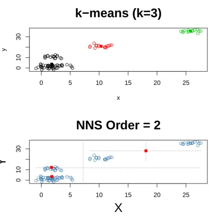
We created a distinctly clustered dataset to present a progression of clusters in Figures 1:3 using 102

the samekfor bothk-means and NNS. 103

0

5

10

15

20

25

0

10

30

k−means (k=1)

x

y

0

5

10

15

20

25

0

10

30

X

Y

NNS Order = 1

(5)

0

5

10

15

20

25

0

10

30

k−means (k=3)

x

y

0

5

10

15

20

25

0

10

30

X

Y

NNS Order = 2

(6)

0

5

10

15

20

25

0

10

30

k−means (k=8)

x

y

0

5

10

15

20

25

0

10

30

X

Y

NNS Order = 3

Figure 3.k=8 fork-means and NNS partitioning. As the number ofkincreases, NNS andk-means will generate more identical points.

Figure1reveals that thek-means cluster and NNS clusters are identical for thek=1 case. Figures 104

2and3depict thek=3, 8 cases. Several shared points in the upper right section of Figures 1 and 3 are 105

visible. 106

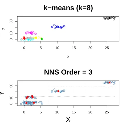
3. NNS Clusters and NNS Regression 107

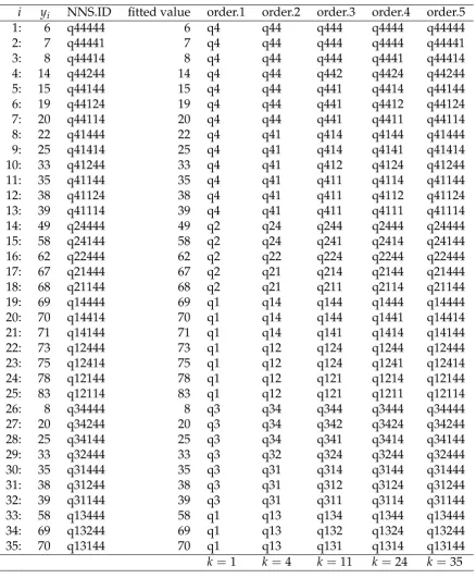
This section explores the relation between NNS clusters and NNS line segments used for curve 108

fitting. Figure 4 displays two columns having three figures each. The original univariate data (provided 109

in the Supplementary MaterialA) are displayed in all six figures, showing a large dip after a peak at 110

x=25. The filled-in squares in all figures represent the cluster means. The right hand figures show 111

regression fit as straight lines joining NNS quadrant (cluster) means equal to ¯X, ¯Yand end points 112

which are determined from another internal NNS algorithm described in [1]. 113

Figure 5 extends the right hand panel of Figure 4 for ordersO= 1, . . . , 5, so that it ultimately 114

(7)

NNS Order = 2

0 5 10 15 20 25 30 35

20

60

NNS Order = 2

Y

R2=1

(9)

The NNS algorithm assigns each observation a special identification number reflecting the 117

quadrant where it ultimately falls. In vector quantization, this step is analogous to the “codebook" 118

which represents the “codevectors". The codevectors are the segment means from a vector quantization 119

partitioning, and are very similar to NNS cluster points as defined above. Again, the primary difference 120

is the lack of an initial specification of a number of desired points for NNS. The sequence of partitioning 121

and assignment of quadrant identifications for each observation is included here for completeness. 122

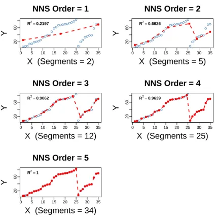
Table 1 presents the special identification numbers for our univariate example in the limit 123

condition, that is forO = 5. Column 1 is the observation number, column entitled “y” has values 124

of the dependent variable, “quadrant” is the sequence of clusters assigned to each observation and 125

the “fitted value” column contains the NNS predictions ˆy. Columns 5:9 are entitled “order.O” for the 126

relevant order and lists the special identification numbers mentioned above. 127

In the third column entitled “quadrant”, the format “q...” describes the sequential partitions. For 128

the first observation, “q44444” was first assigned a partition “4”, as noted in column “order.1”. The 129

final digit 4 is the latest quadrant assignment for the last “order”, which isO=5 here. The bottom 130

row of Table 1 reportsk≤4O−1, the number of nonempty quadrants. 131

The internal NNS numbering of quadrants is not of theoretical significance. NNS uses 1=CUPM 132

(North East quadrant); 2=DUPM (North West quadrant); 3=DLPM (South East quadrant); 4=CLPM 133

(South West quadrant). The rationale behind bookending the CUPM and CLPM with the lowest and 134

highest assignments respectively is computational ease via “min” and “max” commands if those 135

quadrants should be called. For example, our first observation is consistently in the lower left CLPM 136

or fourth quadrant after 5 iterative partitions. These are also used in multivariate dependence defined 137

(10)

Table 1.Quadrant (cluster) identification for univariate example whereO=5. Sequence of quadrant identifications asOincreases andkas the number of non-empty quadrants including endpoints for eachO.

i

y

i

NNS.ID

fitted value

order.1

order.2

order.3

order.4

order.5

1:

6 q44444

6 q4

q44

q444

q4444

q44444

2:

7 q44441

7 q4

q44

q444

q4444

q44441

3:

8 q44414

8 q4

q44

q444

q4441

q44414

4:

14 q44244

14 q4

q44

q442

q4424

q44244

5:

15 q44144

15 q4

q44

q441

q4414

q44144

6:

19 q44124

19 q4

q44

q441

q4412

q44124

7:

20 q44114

20 q4

q44

q441

q4411

q44114

8:

22 q41444

22 q4

q41

q414

q4144

q41444

9:

25 q41414

25 q4

q41

q414

q4141

q41414

10:

33 q41244

33 q4

q41

q412

q4124

q41244

11:

35 q41144

35 q4

q41

q411

q4114

q41144

12:

38 q41124

38 q4

q41

q411

q4112

q41124

13:

39 q41114

39 q4

q41

q411

q4111

q41114

14:

49 q24444

49 q2

q24

q244

q2444

q24444

15:

58 q24144

58 q2

q24

q241

q2414

q24144

16:

62 q22444

62 q2

q22

q224

q2244

q22444

17:

67 q21444

67 q2

q21

q214

q2144

q21444

18:

68 q21144

68 q2

q21

q211

q2114

q21144

19:

69 q14444

69 q1

q14

q144

q1444

q14444

20:

70 q14414

70 q1

q14

q144

q1441

q14414

21:

71 q14144

71 q1

q14

q141

q1414

q14144

22:

73 q12444

73 q1

q12

q124

q1244

q12444

23:

75 q12414

75 q1

q12

q124

q1241

q12414

24:

78 q12144

78 q1

q12

q121

q1214

q12144

25:

83 q12114

83 q1

q12

q121

q1211

q12114

26:

8 q34444

8 q3

q34

q344

q3444

q34444

27:

20 q34244

20 q3

q34

q342

q3424

q34244

28:

25 q34144

25 q3

q34

q341

q3414

q34144

29:

33 q32444

33 q3

q32

q324

q3244

q32444

30:

35 q31444

35 q3

q31

q314

q3144

q31444

31:

38 q31244

38 q3

q31

q312

q3124

q31244

32:

39 q31144

39 q3

q31

q311

q3114

q31144

33:

58 q13444

58 q1

q13

q134

q1344

q13444

34:

69 q13244

69 q1

q13

q132

q1324

q13244

35:

70 q13144

70 q1

q13

q131

q1314

q13144

k

=

1 k

=

4 k

=

11 k

=

24 k

=

35

4. Multivariate Iris Quadrants (Clusters) 139

We use Fisher’s celebrated ‘iris’ dataset using the categorical variable “Species” as the dependent 140

variable to illustrate the multivariate case. 141

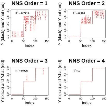
Figure 6 demonstrates the perfect fit and classification achieved by NNS along the bottom right. 142

Since multivariate clusters for four or more regressors cannot be visualized, we presentY and ˆY 143

NNS Order = 4

R2=1

Figure 6. Progression ofOin multivariate NNS fitting. Yand ˆYare displayed (in black and red respectively) for ‘iris’ dataset containing 4 regressors.

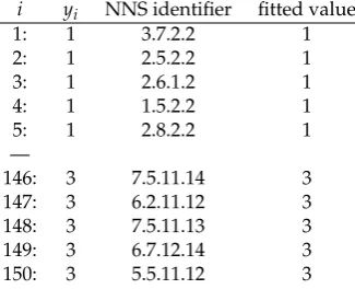
The quadrant identifications assigned by NNS for the corresponding regressor for the iris data are 147

tabulated next. Table 2 shows the truncated output of the multivariate NNS classification usingO=4. 148

Column 1 is the observation number, “y” is the dependent variable representing the 3 species types of 149

iris, “NNS identifier” is the sequence of identifications assigned to each observation and “fitted value” 150

is the NNS prediction of the ‘iris’ dependent variable. 151

The multivariate identifications are not simply quadrant identifications as in the univariate case. 152

These identifications are derived from the “regression point matrix” (RPM) internal to NNS, for ease 153

of reference as suggested by [8]. “Regression points” are the quadrant mean values interpreted as ˆX 154

values derived by NNS for a givenOfor all regressors in theXmatrix. The reader may benefit from 155

(12)

Since ‘iris’ has 4 regressors and 150 observations, the maximum dimensions (in the limit condition 157

whereby every observation is a quadrant mean) of the RPM will be a 150×4 (row-column) matrix. 158

The reason for these alternative identifications is straightforward, efficiency. For 4 regressors, a 159

quadrant identification ofO=4 would require 16 entries of a number 1:4 per the univariate quadrant 160

identification example immediately preceding. Whereby using the RPM, we can assign the uniqueXi 161

identification with much fewer entries even when some or all regressors have double digit entries. If 162

each regressor is aligned with its first regression pointnot partial moment quadrant, each regressor will 163

be assigned a “1”. Thus, we have only 4, not 16 digits in our NNS identifier for multiple regressors. 164

The phrase “unique observation set” refers to the dependent variableyand a matrix of regressors 165

Xfor thei-th observation,(y,X)_iand the identification simply assigns the interval number(1, 2, 3, . . .) 166

along each regressor column in the RPM that correspondingXiis found.X1and the first few rows of

167

RPM are given by: 168

Sepal.Length Sepal.Width Petal.Length Petal.Width

X1 5.1 3.5 1.4 0.2

RPM: 169

Sepal.Length Sepal.Width Petal.Length Petal.Width

1: 4.300000 2.000000 1.0000 0.1000000

2: 4.612500 2.272727 1.3250 0.1852941

3: 5.012000 2.604545 1.5625 0.3000000

4: 5.388889 2.841667 1.9000 0.4000000

5: 5.704762 3.000000 3.2000 0.5500000

6: 6.057895 3.154167 3.5750 1.0000000

Now focus on the first line of Table 2 having the entry: “3.7.2.2” in the “NNS identifier” column. 170

It means the first ‘iris’ regressor “Sepal.length” was assigned a “3”, orx1=1 because its value (5.1)

171

lies within the third interval of[5.012000, 5.388889]of the first column in the RPM; the second regressor 172

“Sepal.Width” a “7”, orx2 = 1 because its value (3.5) corresponded with the 7th interval of the

173

second column in the RPM; the third regressor “Petal.Length” a “2”, orx3=2 because its value (1.4)

174

corresponded with the second interval of the third column; and the final regressor “Petal.Width” a “2”, 175

orx4=2 because its value (0.2) corresponded with the second interval of the fourth column. This set

176

of independent variables corresponded with a “setosa” species. If a new set of measurements matches 177

this partition configuration, NNS will classify it as “setosa”. The reader may immediately recognize 178

the measurement matching technique, as it will generally return the same output as the k-Nearest 179

Neighbors algorithm whenk=1. However, the goal of this paper is to demonstrate NNS as a form 180

of ‘unsupervised learning,’ or clustering. The supervised learning, or classification / multivariate 181

regression features of NNS based on these clusters suggests a strong relationship between NNS and 182

kNN, with notable differences in cluster distance weighting and the lack of restricted cluster sizes for 183

NNS. We leave the full NNS-kNN exposition for another paper. 184

As a further illustration, let us focus on the 5th line of Table 2 with “NNS identifier” value 185

“2.8.2.2” means the first ‘iris’ regressor “Sepal.length” was assigned a “2”, orx1=2 because its value

186

corresponded with the 2nd unique interval of the first column in the RPM; the second regressor 187

“Sepal.Width” was assigned a “8”, orx2=8 corresponding with the 8th interval of the second column

188

in the RPM; the third regressor “Petal.Length” a “2”, orx3=2; and the final regressor “Petal.Width” a

189

“2”, orx4=2. This set of independent variables corresponded with a “setosa” species. If a new set of

190

measurements matches this partition configuration, NNS will classify it as “setosa”. 191

Finally let us focus on the last 150-th line of Table 2 with the “NNS identifier” as “5.5.11.12”. 192

It simply means that the first ‘iris’ regressor “Sepal.length” was assigned a “5”, orx1 = 5 because

193

(13)

RPM; the third regressor “Petal.Length” equals “11”, orx3=11; and the final regressor “Petal.Width”

196

equals “12”, orx4=12. This set of independent variables corresponded with a “virginica” species. If a

197

new set of measurements matches this partition configuration, NNS will classify it as “virginica”. The 198

full table is obtained by a one-line R command from the NNS package provided in the Supplementary 199

MaterialA. 200

Table 2.Multivariate NNS partitioning and NNS.ID assignments for ‘iris’ dataset forO=4

i yi NNS identifier fitted value

1: 1 3.7.2.2 1

2: 1 2.5.2.2 1

3: 1 2.6.1.2 1

4: 1 1.5.2.2 1

5: 1 2.8.2.2 1

—

146: 3 7.5.11.14 3

147: 3 6.2.11.12 3

148: 3 7.5.11.13 3

149: 3 6.7.12.14 3

150: 3 5.5.11.12 3

Table 2 shows that the categorical variableyand the fitted value ˆyare identical, as does theR2

201

Figure6, proving a perfect fit in a finite order by NNS for the iris data. 202

4.1. Additional Visualizations 203

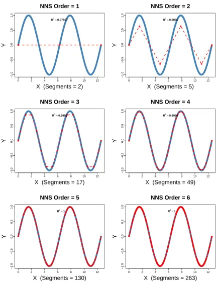
We present a univariate and multivariate 3d visualization of the progression of NNS fitting. 204

4.1.1. Univariate 205

The following R code is used to generate an NNS fit of increasing orders on a periodic sine wave. 206

Y

R2=1

Figure 7.Progression ofOin univariate NNS curve fitting of periodic sine wave.

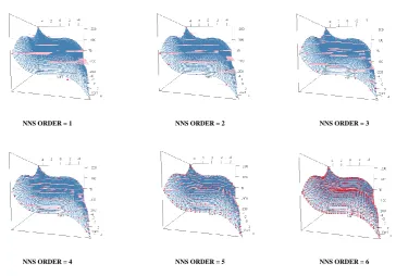
4.1.2. Multivariate 209

The following R code is used to generate an NNS fit of increasing orders on a nonlinear 210

multivariate function. 211

f <- function(x, y) x^3+3*y-y^3-3*x 212

(15)

g <- f(z[,1],z[,2]) 215

for(i in 1:6){NNS.reg(z,g,order=i)} 216

NNS ORDER = 1 NNS ORDER = 2 NNS ORDER = 3

NNS ORDER = 4 NNS ORDER = 5 NNS ORDER = 6

Figure 8.Progression ofOin multivariate NNS curve fitting of nonlinear function. Red dots are NNS quadrant means and pink “plates” are regressor regions covered by specific NNS quadrant.

5. Conclusion 217

In conclusion, curve fitting is an old and important problem with a long history. High order 218

polynomials and kernel regressions are intrinsically approximate. This paper uses artificial univariate 219

y= f(x)data and the well-known multivariate iris data to illustrate and display how a newer NNS 220

algorithm reaches a perfect fit while using quadrants as clusters along the way. We offer analogies 221

to existing techniques such ask-means and codevectors when defining NNS clusters and explain 222

the differences in objective functions / initial parameter specifications. We also illustrate quadrant 223

identifiers internal to NNS for univariate and multivariate cases which help speed the algorithm. 224

The perfect fit in finite steps is not claimed to be directly usable in practice since some noise 225

is always present. In sampling theory sample size is sometimes determined after specifying the 226

error rate, which is possible because the perfect result (exact value of the population parameter) is 227

potentially available. We are currently working on extending NNS to nonparametric regressions, 228

providing a similar capability to first choose an error rate and then obtain a nonparametric fit. All 229

this is now feasible due to the perfect fit in relatively simple finite steps described here. In any case, 230

NNS fills a gap in the nonparametric regression literature by offering flexibility which in turn yields 231

high quality interpolation and extrapolation from a nonparametric fit illustrated in [1]. The NNS 232

(16)

identifier matrix serves the same purpose as vector quantization codebooks. Thus NNS shares a lot of 234

features with some very robust long-standing techniques while offering a slew of additional features 235

in a convenient R package. 236

Appendix. Supplemental R-Code 237

We provide all of the R-code used to produce the above examples and plots. Sincek-means is not 238

deterministic, the clustering examples may not replicate exactly to what is presented above but should 239

still sufficiently highlight the differences in objective functions. Note that the typical code involves 240

very few lines. 241

Clustered Dataset: 242

n = 100;g=6;set.seed(g) 243

d <- data.frame(x = unlist(lapply(1:g, function(i) rnorm(n/g, runif(1)*i^2))), 244

y = unlist(lapply(1:g, function(i) rnorm(n/g, runif(1)*i^2)))) 245

Figure 1 R-commands: 246

require(NNS); require(clue) 247

par(mfrow=c(2,1)) 248

plot(d, col = kmeans(d,1)$cluster, main=paste("k-means (k=",1,")",sep = ""), 249

cex.main=2) 250

points(kmeans(d,1)$centers,pch=15,col=1) 251

NNS.part(d$x,d$y,order=1,Voronoi = T) 252

cex.main=2) 256

points(kmeans(d,3)$centers,pch=15,col=1:3) 257

NNS.part(d$x,d$y,order=2,Voronoi = T,noise.reduction = ’off’) 258

cex.main=2) 262

points(kmeans(d,8)$centers,pch=15,col=1:8) 263

NNS.part(d$x,d$y,order=3,Voronoi = T,noise.reduction = ’off’) 264

Univariate Data Example R-command: 265

set.seed(345);x=sample(1:90);y1=sort(x[1:25]);y2=sort(x[1:10]);y=c(y1,y2);xx=1:35 266

for(i in 1:3){NNS.part(xx,y,order=i,Voronoi=T,noise.reduction = ’off’); 269

NNS.reg(xx,y,order=i,noise.reduction = ’off’)} 270

for(i in 1:5){NNS.reg(xx,y,order=i,noise.reduction = ’off’)} 273

(17)

for(i in 1:4){NNS.reg(iris[,1:4],iris[,5],order=i)} 276

RPM R-commands: 277

head(NNS.reg(iris[,1:4],iris[,5],order=4)$rhs.partition) 278

Table 1 R-commands: 279

order=matrix(nrow=35,ncol=5) 280

colnames(order)=c("order.1","order.2","order.3","order.4","order.5") 281

for(i in 1:5){order[,i]= 282

NNS.reg(xx,y,order=i,noise.reduction = ’off’)$Fitted.xy[,NNS.ID]} 283

cbind(NNS.reg(xx,y,order=5,noise.reduction = ’off’)$Fitted.xy[,.(y,NNS.ID)],order) 284

Table 2 R-commands: 285

NNS.reg(iris[,1:4],iris[,5],order=4)$Fitted.xy[,.(y,NNS.ID,y.hat)] 286

Even though the paper does not discuss extrapolation and interpolation of fitted nonparametric 287

regression functions in detail, the following code illustrates the ease with which these tasks are 288

implemented. (i) Interpolation and extrapolation for artificial data are illustrated by following 289

commands: 290

NNS.reg(xx,y,noise.reduction = NULL,point.est = 25.5) 291

NNS.reg(xx,y,noise.reduction = NULL,point.est = 36) 292

(ii) Illustrative Iris data interpolation and extrapolation commands are: 293

NNS.reg(iris[,1:4],iris[,5],point.est = (iris[1,1:4]+.01))$Point.est 294

NNS.reg(iris[,1:4],iris[,5],point.est = (iris[150,1:4]+1))$Point.est 295

296

1. Vinod, H.D.; Viole, F. Nonparametric Regression Using Clusters. Computational Economics, June 19, 2017 297

2017.

298

2. Viole, F.; Nawrocki, D. Deriving Nonlinear Correlation Coefficients from Partial Moments.SSRN eLibrary 299

2012.

300

3. Hayfield, T.; Racine, J.S. Nonparametric Econometrics: The np Package. Journal of Statistical Software2008,

301

27, 1–32.

302

4. Kohonen, T. The Self-organizing Map. Proceedings of the IEEE1990,78, 1464–1480.

303

5. Grbovic, M.; Vucetic, S. Regression Learning Vector Quantization. IEEE International Conference on Data 304

Mining (ICDM)2009, pp. 788–793.

305

6. Viole, F.NNS: Nonlinear Nonparametric Statistics, 2016. R package version 0.3.6.

306

7. Viole, F. Beyond Correlation: Using the Elements of Variance for Conditional Means and Probabilities.

307

SSRN eLibrary2016.

308

8. Bellman, R. On the approximation of curves by line segments using dynamic programming.

309

Communications of the ACM1961,4, 284.