Characterizing complex mineral structures in thin
section of geological sample with a scanning Hall effect
microscope
Jefferson F. D. F. Araujo1,*, Andre L. A. dos Reis2, Vanderlei C. Oliveia Jr.2, Amanda F. Santos3, Cleanio Luz-Lima4, Elder Yokoyama5, Leonardo A. F. Mendozaand6, João M. Perreira7 and Antonio C. Bruno1
1 Department of Physics, Pontifical Catholic University of Rio de Janeiro, Rio de Janeiro 22451–900, Brazil; [email protected]
2 Department of Geophysics, Observatório Nacional, Rio de Janeiro, Brazil; [email protected] (A. R.); [email protected] (V. O.)
3 Department of Physics, University of California, Santa Barbara, California 93106, USA; [email protected]
4 Department of Physics, Campus Ministro Petrônio Portella, Universidade Federal do Piauí, Teresina 64.049-550, PI, Brazil; [email protected]
5 Institute of Geosciences, University of Brasília, Brasília, Brazil; [email protected]
6 Department of Electrical Engineering, Universidade Estadual do Rio de Janeiro, Rio de Janeiro 20550- 900, Brazil; [email protected]
7 Fiber Optics, RISE Acreo, Electrum 236, 164 40, Kista, Sweden; [email protected] * Correspondence: [email protected]; Tel.:+55-21-3527-1260
Abstract
:
We improved a magnetic scanning microscope for measuring the magnetic properties of minerals in thin sections of geological samples at submillimeter scales. The microscope is comprised of a 200 µm diameter Hall sensor that is 142 µm from the sample; an electromagnet capable of applying to the sample up to 500 mT dc magnetic fields over a 40 mm diameter region; a second Hall sensor arranged in a gradiometric configuration to cancel the background signal applied by the electromagnet and reduce overall noise in the system; a custom-designed electronics to bias the sensors and provide adjustment for background signal cancelation; and a scanning XY stage with micrometer resolution. Our system achieves a spatial resolution of 220 µm with noise at 6.0 Hz of 300 nTrms/(Hz)1/2 in an unshielded environment. The magnetic moment sensitivity is 1.3 × 10⁻¹¹ Am2. We successfully measured the representative magnetization of a geological sample using an alternative model that takes into account the sample geometry and identified different micrometric characteristics in the sample slice.Keywords:Magnetic scanning microscope; Hall sensor; Magnetic materials; Geological sample
1. Introduction
Scanning magnetic microscopy has attracted much interest in recent years; it has the potential to elucidate a number of problems in science and engineering involving magnetization images [1-4]. Applications involving scanning magnetic microscopy cover many disciplines, from physics and material
science [5-8] to paleomagnetism, magnetism [9-10] and biophysics [11-13]. In paleomagnetism, for example, scanning magnetic microscopy can be used to recover information about past magnetic fields by analyzing the magnetizations of terrestrial or extraterrestrial rocks. Such rocks or meteorites can hold magnetic information for millions, or even billions of years; however, the record of the oldest magnetic fields is commonly superimposed by other magnetic records acquired during the geological history of the material. Classical paleomagnetic techniques are based on the external measurement of the sample’s magnetic field. Thus, they reflect the vector sum of the magnetic moments of all rock minerals measuring a bulk magnetization of a cylindrical sample. In particular, rocks that have developed complex structures, such as breccied rocks, folded rocks and sedimentary rocks, may be particularly difficult to analyze by conventional paleomagnetic techniques [14].
Scanning magnetic microscopes make up a new class of magnetometers capable of producing magnetic field maps with submillimeter spatial resolution. Broadly, a sample is moved horizontally under a tiny magnetic sensor located very close to the surface of the sample. A magnetic map is then constructed by recording the measurement of the magnetic field at each point of a regular grid of positions [1-7,15-18]. Additionally, the majority of magnetic microscopes operate at low temperatures, because they use SQUID (Superconducting Quantum Interference Device) sensors and magnetic shielding due to the sensitivity of the reading systems [16-18].
With this objective, we developed a magnetic microscope which performs magnetic mapping at ambient temperature with a large scanning area and the ability to handle samples in the millimeter scale, in addition to being able to identify distinct constituents of complex structures. The microscope has a small electromagnet that can apply a uniform DC magnetic field up to 500 mT perpendicular to the sample. In the current configuration, the scanning magnetic microscope is equipped with a pair of low-cost commercial Hall effect sensors, thus forming an axial gradiometer. The gradiometer serves a dual purpose to cancel the magnetic field applied by the electromagnet and reduce the ambient magnetic noise since it operates in an unprotected environment. The sensitivity of the magnetic moment reached (1.3 × 10⁻¹¹ Am2) can allow for the study of the geological samples, solid samples, liquids, microstructures and nanostructured samples. Furthermore, the spatial resolution of the current sensor (200 µm) can allow for the measurement of magnetic maps in different regions of the same sample. Through these maps, the sample is characterized in different positions, showing, in the case of the geological samples, that there are different minerals within the same sample.
2.Scanning Magnetic Microscope
2.1 Mechanical design
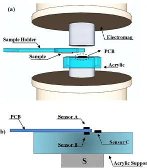
sample is placed upside down in the sample holder using double-sided adhesive tape. For sensing the response generated by the sample to the applied field, we use two commercial Hall sensors HQ-811 (AKM, Corp), henceforth designated Sensor A and Sensor B, which incorporate an InAs element in a SMT package (Figure1b). Their 200 m diameter sensing areas have a nominal distance of 142 m to the top surface. The two sensors are connected in an axial gradiometric configuration and fixed on opposite sides of a 2.2 mm thick printed circuit board (PCB).
Figure 1. (a) Schematic drawing of the main components of the microscope: north and south pole of the
electromagnet, an acrylic holder containing the PCB board with Hall effect sensors, a sample holder that moves in the X and Y directions and sample. Drawing is not to scale. (b) PCB board details containing the gradiometric sensors (A and B), additional sensor (C) for measuring the applied field and sample holder.
sensor and the top surface as 150 m. Further lapping will prevent the sensor from working properly. The PCB is mounted on an acrylic structure that is fixed to one of the electromagnetic poles. For Sensor C, the programmable linear Hall sensor MLX-90215 was used and glued to the acrylic support.
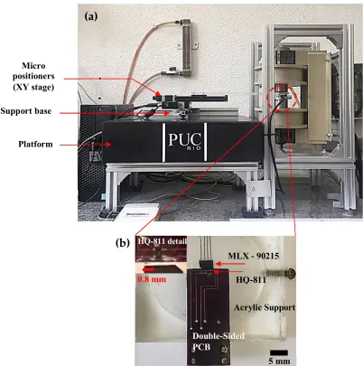
Figure 2. (a) Photo of the magnetic scanning microscope. (b) Photo of the Hall sensors and acrylic structure that fits
around one electromagnetic pole. Two HQ-811 sensors in each side of the PCB form an axial gradiometer. The MLX-90215 measures the applied field. At the top, we have the increment. We can check details of the connection of the HQ-811 photo sensor with scale.
2.2 Custom electronics
We can bias the HQ-811 sensors by current or voltage. After several tests, we concluded that biasing by current in the 1 – 5 mA range produced the best signal-to-noise ratio. The circuit built consisted of two independent current sources and instrumentation amplifiers for signal amplification and
MLX - 90215
HQ-811 HQ-811 detail
Acrylic Support
Double-Sided PCB
5 mm
0.8 mm
Micro positioners (XY stage)
Support base
Platform
(a)
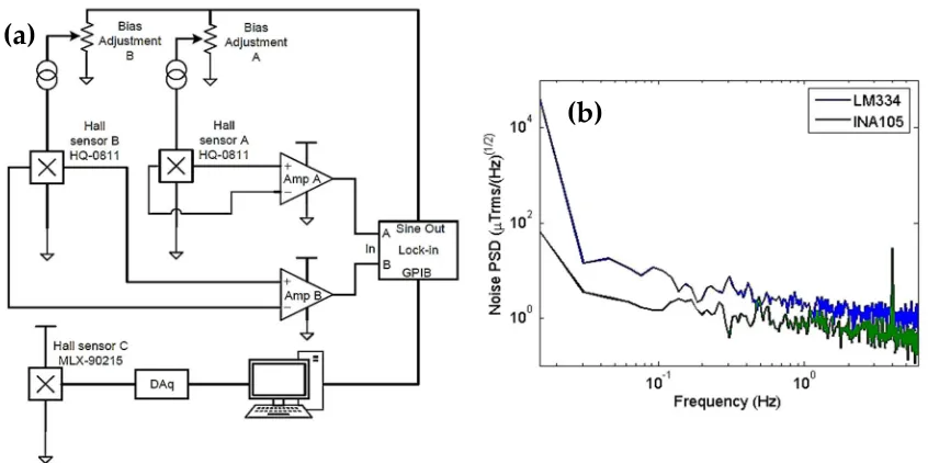
decoupling (see Figure 3a). A low-noise preamplifier (SR560, SRS Inc.) accomplishes the gradiometer operation by electronically subtracting the two output signals. In the first version, the current sources were based on the IC LM334 and controlled by resistance, showing a high noise and strong temperature dependence, even when using a temperature compensation circuit [19]. Then, we redesigned the circuit by replacing the LM334, for the two current sources that are controlled by voltage with the INA105. This redesign attained better results. Figure3b shows a comparison between the noise of the two custom electronics.
Figure 3. (a) Electronics using the INA105 schematics for currents sources and preamplification for the Hall
gradiometer. (b) Noise spectrum of the HQ-811 sensor with two custom electronics measured outside a magnetic shield in the laboratory. For comparison purposes, a magnetic signal at 4 Hz with 5 µT peak amplitude was added to the measurements. The noise level at 6 Hz is approximately 300 nTrms/√Hz.
We used a biasing AC current at 1.0 kHz frequency and a peak amplitude of 1.0 V. For comparison purposes, we added to the measurements a magnetic signal at 4 Hz with a 5 µT peak amplitude. The spectrum indicated by the legend INA105, shows a noise level at 6 Hz of approximately 300 nTrms/√Hz. We designed the gradiometer primarily for rejecting the applied field, increasing the dynamic range of the instrument and allowing its operation at high applied fields. However, the gradiometer also rejects the ambient magnetic noise. The applied field rejection was tuned by applying a uniform field of 500 mT and then adjusting the biasing current of Sensor B until the output read 0.5 mT, a factor of 1.000 in field rejection. Afterwards, to evaluate the effect on the magnetic noise, we measured a sample consisting of a cavity with 500 µm diameter and 400 µm depth and filled with 99.9% pure magnetite (Fe3O4) fine particles, a mass of 102 µg was used. Due to the proximity of the sample port to the sensors, the best model to fit the experimental curves is a current cylinder, because the cavity where the sample is deposited has the shape of a cylinder. Assuming that our sample consists of fine particles and completely fills the cavity, it has a magnetic moment (mz), which is uniformly distributed in the z-direction (the
(a)
magnetic field applied by the electromagnet H has the same direction), radius a and compliment of 1. The z-component of the field can be obtained using the Biot-Savart law [20-21]. By measuring Bz for several values of applied field, using (x ', y', z’) obtained with the aid of an optical microscope and using the sensor plug, it was possible to estimate these relative distances between the center of the sample holder and the center of the active part inside the sensor. Therefore, we can obtain the magnetic moment as a function of the applied field according to the equation below [21]:
'
,
'
,
'
'
cos
)
'
(
4
)
(
2 0 3 2 / 2 / 0 2 2z
y
x
B
dz
d
r
a
z
z
l
a
H
m
z l l z
(1) 'r the distance between the element is defined
r
'
(
x
'
x
)
2
y
'
asen
2
z
'
a
cos
2
1/2,already
d
l
is the distance between the element and the point p in space XY
d
l
a
d
j
cos
, µ0is the permeability of the free space and the radius of a cylinder uniformly magnetized along its length l. We can determine the real z distance between the sample and the sensor by scanning a line at the top of the sample Bz = (x ', y', z ') and analyzing only the spatial dependence of Bz with a = 500 µm, l = 400 µm. Using a least square fitting routine, we obtained 142 µm for the actual distance from the Hall sensor element to the top of the sample. Using this distance and 5197 kg/m3 for Fe3O4 bulk density, we found 75.8 Am2/kg for the magnetization at 500 mT, about 0.19% greater than the value obtained in the Vibrating-sample magnetometer (VSM) and 0.23% less than the value obtained in the Hall magnetometer [22-24].
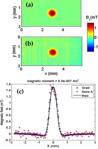
We compared the gradiometer and top sensor (Sensor A) outputs. The results, shown in Figure
Figure 4. Gradiometer test with a sample consisting of a cavity with 500 µm diameter, 400 µm depth and filled with
99.9% pure magnetite, approximately 102 µg. (a) Map of the remanent field with the gradiometer turned on. (b) Map with only Sensor A. (c) The plot shows the theoretical field due the magnetite sample (solid line), measured by the gradiometer (circles) and measured by sensor A (crosses).
3.Measurement of geological samples
3.1 Microscopy of geological samples
To demonstrate the characterization abilities of our magnetic microscope, we mapped a geological sample typical of the ones found at Jack Hills. The Jack Hills is a 70 km long range of hills located on southern margin of Narryer Terrane, Western Australia [25]. It comprises an Archean-Paleoproterozoic greenstone belt that is surrounded by granitic and gneissic rocks. The greenstone belt is a sequence of metavolcanic and metasedimentary rocks that usually have a polycycle history of metamorphism and deformation. A diminute part of the Jack Hills greenstone belt is composed of banded iron- formation (BIF) that records much of deformation history [26]. According to Spaggiari (2007) this BIF can preserve at least three generation of folding deformation that can be observed both meso and micro scales.
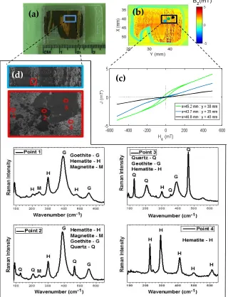
To demonstrate the capability of our microscope, we scanned a polished section of Jack Hills BIF sample. This sample shows a microfold of alternating microbands of iron oxi-hydroxides and silica (see Figure5a). The Figure5b shows the perpendicular component of the magnetic field response of a 20 × 25 mm scan of the microfold sample, in the presence of a 500 mT field applied perpendicular to the sample and observed three points. The first point, in blue color, is located in x = 43.7 mm and y = 35 mm, the
(a)
(b)
second point, in green color, is located in x = 45.2 mm and y =38 mm and the last third point, in black color, is located in x = 46.8 mm and y = 40 mm.
Figure 5. (a) Photo of the microfold structure attached in the sample port. (b) The perpendicular component of the
magnetic field response of a 20 × 25 mm scan of the microfold sample, in the presence of a 500 mT field applied, we can see the three point. The first point, in blue color, is located at x = 43.7 mm and y = 35 mm; the second point, in green color, is located at x = 45.2 and y = 38 mm; and the third point, in black color, is located at x = 46.8 mm and y = 40 mm. (c) Hysteresis cycle curves of the induced magnetic field J(mT) at the three points of the sample, also indicating through the curves that there are different minerals. (d) We have in figure images made in scanning electrocine microscopy of a line. Within this line 4 points were identified in different positions and analyzed by Raman spectroscopy and the results of these points 1, 2, 3 and 4 different minerals were identified in the same sample.
(a)
(b)
(c)
The Figure5c show three curves of a hysteresis cycle at the three different fixed points of the same sample shown in Figure 5b. The curves represents the magnetic response of the induced field of the sample, which were obtained by positioning the sample in the points of the Figure5b in relation to the sensitivity axis of the microscope reading system made in the position of the red point. We observed that these are different curves, therefore, they represent different minerals within the same sample. This type of study cannot be done with conventional magnetometers because the sample is treated as being evenly distributed [20,22-24]. In order to verify the presence of different minerals we performed an Raman spectroscopy analysis of a small region of the sample (see Figure5a and Figure5d). Raman measurements were performed using a micro-Raman Senterra Bruker spectrometer, and the 785 nm line of a laser was used as the excitation source. The spectrometer slit was set for a resolution of 4 cm-1. An optical microscope (Olympus BX-50) with Olympus MPlan N 20x/0.40NA Objective was used to focus the laser on the sample surface and to obtain the images, Figure5d. In this figure we select a rectangle marking a new region, which brings small circles numbered from 1 to 4. These circles show where the Raman spectra of the sample identified as: Point 1, Point 2, Point 3 and Point 4 were obtained. When we analyzed the spectra obtained, we observed that the predominant concentration in the sample is of hematite and quartz respectively, this assertion is due to the fact that characteristic peaks of these phases are observed in the other spectra, but besides these phases were also observed the phases geothite and magnetite.
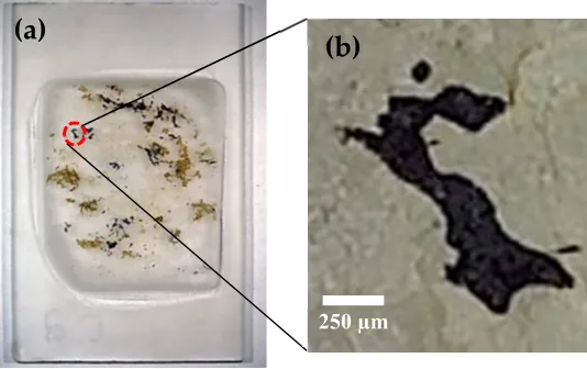
Besides of Jack Hills BIF we scanned a sample of metamorphic rock from the 300 km diameter Vredefort Dome in South Africa. Vredefort Dome is a 90-km-wide central uplifted of a 300-km-wide eroded impact structure [e.g., 27]. The exposed Vredefort central uplift comprises polydeformed Archean migmatitic gneisses and granitoids with scattering occurrence of metasedimentary and mafic granulite xenoliths [27]. The sample in the form of a 30 µm thin section (see Figure6a and Figure6b) was prepared from a core drilled in granulite-gneiss within the 9 × 9 m2 and the dark regions contains magnetic carriers and are surrounded by nonmagnetic plagioclase feldspar and quartz [28]. Figure 6b shows a picture, taken with an optical microscope, of a small region of the thin section denoted ‘hook’ in the picture of the slice.
Figure 6. (a) Vredefort thin section. (b) Shows a picture, taken with an optical microscope.
(a)
(b)
3.2 Modeling using current circuit
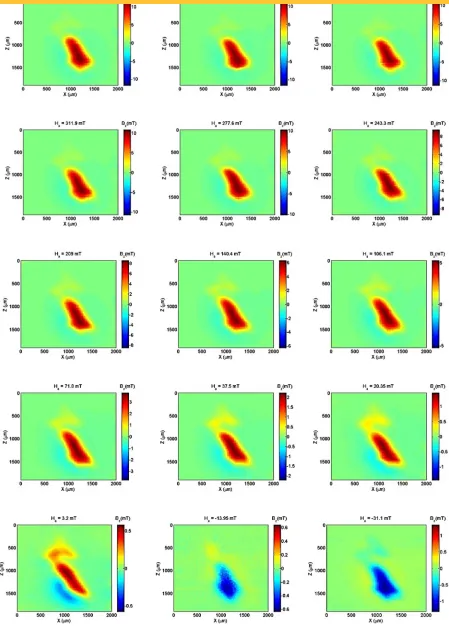
We imparted on the sample magnetic fields varying from 415 mT to –31 mT. Figure7shows a set of 15 experimental Bz maps (25 µm step) of the hook for each applied magnetic field. From the maps, a weak contribution from the upper part of the hook is observed that we termed the ‘head’. The main body (‘handle’) of the hook presents a stronger magnetic field response. A model is needed to characterize these two regions of the sample. The model of a single dipole is useful when the sample is distant or when it has a spherical shape. This is not the case with this microscope because the sensor is very close to the sample. For this case, the current circuit model was developed, assuming both head and handle. The calculation starts from the law of Biot-Savart (see Equation (2)):
'
'
'
4
'
,
'
,
'
0 2r
r
r
l
d
I
z
y
x
B
loop z
(2)where I is the current in the circuit and dl is the element of length on which the integral along the area of the sample is calculated. The induced field of the sample in the presence of the applied field is acquired directly from the map, which is measured in the scanning magnetic microscope. Therefore, by knowing the Bz(x’,y’,z’) and taking the area of the sample, we can extend the value of the current through Equation (3). If the current is confined in an XY plane and the reading in the z-direction the magnetic moment can be represented as follows:
m
z
I
(
Area
)
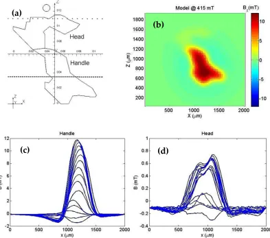
(3)To quantify these two main contributions for the detected magnetic field, we used the two current loop model in the shape of the hook, as shown in Figure8a. We called the top loop the “head” and the bottom loop the “handle”. Figure8b shows the simulated perpendicular component of the field for a 415 mT applied field. Note that Bz in the model coincides with Bz as measured experimentally (See Figure7 ~ 415 mT).
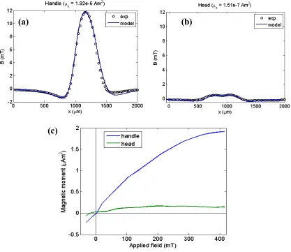
Figure 8. (a) Current loop model divided in two parts: the “handle” (high current) and “head” (low current). The scale is in cm. (b) Simulated By map with the current loop model. (c) By measured over the dashed line Z=350 µm for different applied fields. (d) By measured over the dotted line Z=1100 µm for different applied fields.
To find the current in each loop that adjusts the magnetic field generated by the model to the experimental field, we used the field along the dotted line (Z = 1100 µm) for the “head” and the field along the dashed line (Z = 350 µm) for the “handle”, as shown in Figure8a, Figure8c and Figure8d show the perpendicular magnetic field component at each of the lines for the different values of applied field in the handle and head regions, respectively. Figure9a and Figure9b show the fitting results for 415 mT, using the model of a current circuit. The current values found times the area of each loop is the magnetic moment
(a)
(b)
of each part of the hook. For the “handle”, = 1.92 × 10 , and for the “head”, = 1.51 × 10 .
Figure 9. (a) Model fitting with experimental data over Z = 350 µm for highest applied field. (b) fitting with
experimental data over Z = 1100 µm for highest applied field. (c) Magnetization curves for the two parts of the hook.
Finally, Figure9c shows the magnetization curves for each part of the hook, suggesting that these parts may be composed by different minerals.
3.3 Modeling using polygonal prisms
In order to investigate the contribution of the two parts of the hook (i.e., head and handle), a different approach can be applied from that which was used in the previous section (current circuit). This approach is based on a methodology widely used in geophysics for modeling of potential fields proposed by Plouff [29]. It calculates the potential field of a 3D prism with polygonal cross-section.
(a)
(b)
Let be do an N-dimensional vector whose ith element is the vertical component of magnetic field produced by a magnetic source in the position (xi; yi; zi) (Figure10a). By considering that the sample can be approximated by a set of L polygonal prisms, positioned according a right-handed Cartesian coordinate system and considering x-, y- and z-axis positively oriented to north, east and downward, respectively. We assume that each prism represents different homogeneously magnetized region and the edges coincide with the bounds of the hook. We can estimate the magnetic moment mk, k = 1,…,L, by comparing the synthetic data produced by the model and the vertical component of the magnetic field map measured by the magnetic microscopy, since the sensor-to-sample distance, the thickness of thin section and magnetization direction are known. Mathematically, the vertical component of magnetic field Bz produced
by a set of polygonal prisms at the point (xi; yi; zi) is given by;
,
,
B
=
b
(x
i,
y
i,
z
i,
x
k,
y
k,
m
ˆ
k,
m
k,
z)
L 1 k ik z i z
i i iz
x
y
z
B
(4)where
b
ikz represents the effect of the kth prism at the ith point (xi; yi; zi), xk is a vector containingx-coordinates of the vertices of kth prism, yk is a vector containing y-coordinates of the vertices of kth prism,
k
mˆ is a unit vector in the direction of magnetization,
m
k is the magnetization intensity and Δz is the thickness of each prism. Mathematically, the vertical component of magnetic field produced by the kth prism is given by the expression
b
ikz
C
mM
ikm
ˆ
km
k (5)where Cm is a constant proportional to free space permeability and
zz ik T
ik yz ik xz ik
M
z
)
[
]
,
y
,
x
,
z
,
y
,
(x
M
i i i k k
(6)where the scalar function
ikis given by
k v k ik ikdv
r
1
(7)and
r
ik
(x
i
k)
2
(y
i
k)
2
(
z
i
k)
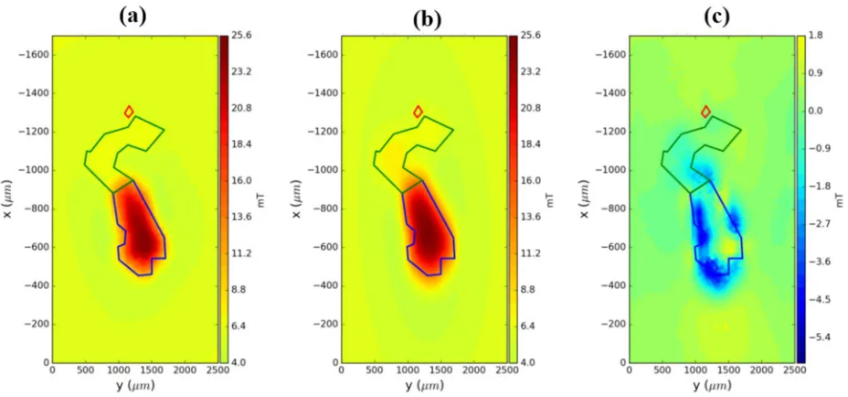
2 (8)to estimate the two main contributions of the hook, we approximate the sample by three polygonal prisms with thickness Δz = 30 µm and vertices showed in Figure10b. We generate the vertical component of magnetic field of the model (Figure10c). As we note in Figure10, the observed data and the synthetic data produced by modeling are very similar. The magnetic moment estimated for head part (green prism in Figure10b) is mhead = 1.89 x 10⁻⁷Am2 and the magnetic moment for handle part (blue prism in Figure10b) is
mhandle = 2.52 x 10⁻⁶Am2.
Figure 10. Comparison between synthetic data and observed data for vredefort thin section. (a) Observed data from
magnetic microscopy of the hook in vredefort thin section. (b) Sample bounds formed by a set of polygonal prisms, in red is the head part of the hook and in blue is the handle part of the hook. (c) Synthetic data generated using Plouff [26].
These results are in the same order of magnitude as the results obtained using a current circuit model (See Figure 9c). So, we can notice that the results using polygonal prisms are consistent by comparing with the current circuit modeling.
4. Conclusion
of 100 to 100 mm. The sensors were configured as axial gradiometer that successfully reduced both applied field and magnetic noise in the output signal.
We successfully measured the representative magnetization of the geological sample using an alternative model that takes into account the sample geometry and identified different micrometric characteristics in the sample slice. The model used was confronted with another model using polygonal prisms resulting in very similar magnetization values.
Author Contributions: Data curation, J.A., A.R., V.O. and A.S.; Methodology, J.A., C.L., E.Y. and A.B.; Software, A.R.
and V.O.; Validation, L.M. and J.P.; Writing, review, & editing, J.A., A.B.
Funding: This study was funded in part by the following Brazilian agencies: The National Council for Scientific and
Technological Development (Conselho Nacional de Desenvolvimento Científico e Tecnológico – CNPq), the Coordinating Agency for the Improvement of Higher Education (Coordenação de Aperfeicoamento de Pessoal de Nível Superior – Capes) and the Research Support Foundation of Rio de Janeiro (Fundação de Amparo à Pesquisa do Estado do Rio de Janeiro – FAPERJ).
Acknowledgments: We thank Professors Benjamin Weiss and Eduardo Andrade de Lima both of the Department of
Planetary Sciences at the Massachusetts Institute of Technology for providing the geological samples and Fredy Osorio for assistance in drawing Figure 5c.
Conflicts of Interest:The authors declare no conflict of interest.
References
1. He, D.; Shiwa, M. A magnetic sensor with amorphous wire. Sensors 2014, 14, 10644–10649. doi: 10.3390/s140610644
2. Rudge, J.; Xu, H.; Kolthammer, J.; Hong, Y.K.; Choi, B.C. Sub-nanosecond time-resolved near-field scanning magneto-optical microscope. Rev. Sci. Instrum. 2015, 86, 023703–23705. doi: 10.1063/1.4907712
3. Shaw, G.; Kramer R.B.G.; Dempsey, N.M.; Hasselbach, K. A scanning Hall probe microscope for high resolution, large area, variable height magnetic field imaging. Rev. Sci.
Instrum. 2016, 87, 113702–113710. doi: 10.1063/1.4967235
4. Kirtley, J.R.; Paulius, L.; Rosenberg, A.J.; Palmstrom, J.C.; Holland, C.M.; Spanton, E.M.; Schiessl, D.; Jermain, C.L.; Gibbons, J.; Fung, Y.K.K.; Huber, M.E.; Ralph, D.C.; Ketchen, M.B.; Gibson, G .W.; Moler, K.A. Scanning SQUID susceptometers with sub-micron spatial resolution. Rev. Sci. Instrum. 2016, 87, 093702– 93711. doi: 10.1063/1.4961982
5. Yamamoto, S. Y.; Schultz, S. Scanning magnetoresistance microscopy. Appl. Phys. Lett. 1996, 69, 3263–5. doi: 10.1063/1.118030
7. Schrag, B. D.; Xiao, G. Submicron electrical current density imaging of embedded microstructures. Appl. Phys. Lett. 2003, 82, 3272–4. doi: 10.1063/1.1570499
8. Schrag, B. D.; Liu, X. Y.; Shen, W. F.; Xiao, G. Current density mapping and pinhole imaging in magnetic tunnel junctions via scanning magnetic microscopy. Appl. Phys.
Lett. 2004, 84, 2937–9. doi: 10.1063/1.1695194
9. Reis, A.L.A.; Oliveira Jr, V.C.; Yokoyama, E.; Bruno, A.C.; Pereira J. M. B. Estimating the magnetization distribution within rectangular rock samples. Geochem. Geophys. Geosyst. 2016, 17, 3350-3374. doi: 10.1002/2016GC006329
10. Kletetschka, G.; Schnabl, P.; Šifnerová K.; Tasáryová Z.; Manda, S.; Pruner P.; Magnetic scanning and interpretation of paleomagnetic data from Prague Synform’s volcanics.
Studia Geophysica et Geodaetica 2013, 57, 103-117. doi: 10.1007/s11200-012-0723-4
11. Chieh, J.; Wei, W.; Liao, S.; Chen, H.; Lee, Y. ; Lin, F.; Chiang, M.; Chiu, M.; Horng, H.; Yang, S. Eight-Channel AC magnetosusceptometer of magnetic nanoparticles for
high-throughput and ultra-high-sensitivity immunoassay. Sensors 2018, 18, 1043-1052. doi: 10.3390/s18041043
12. Parra, A. C.; Casper F.; Paul J.; Lehndorff R.; Haupt C.; Jakob G.; Kläui M.; Hillebrands B. Microstructure design for fast lifetime measurements of magnetic tunneling junctions.
Sensors 2019, 19, 583-591. doi: 10.3390/s19030583
13. Chemla, Y. R.; Grossman, H. L.; Poon, Y.; McDermott R.; Stevens R.; Alper, M.D.; Clarke, Ultrasensitive magnetic biosensor for homogeneous immunoassay. P.N.A.S. 2000, 97, 14268-14272. doi: 10.1073/pnas.97.26.14268
14. Noguchi, Y.; Yuan, Z.; Bai, L.; Schneider, S.; Zhao, G.; Stillman, B.; Speck, C.; Li, H.; Cryo-EM structure of Mcm2-7 double hexamer on DNA suggests a lagging-strand DNA extrusion model. P.N.A.S. 2017, 26, E9529-9. doi: 10.1073/pnas.1712537114
15. Weiss, B.P.; Fu, R.R.; Kehayias, P.; Bell, E.A.; Gelb, J.; Araujo, J. F. D. F.; Lima, E.A.; Borlina, C.S.; Boehnke, P.; Harrison, T.M.; Richard, J.H.; Walsworth, R.L. Secondary magnetic inclusions in detrital zircons from the Jack Hills, Western Australia, and implications for
the origin of the geodynamo. Geological Society of America 2018, 46, 427-433. doi: 10.1130/G39938.1
16. Faley, M.I.; Kostyurina, E.A.; Kalashnikov, K. V.; Maslennikov, Yu. V.; Koshelets, V. P.; Dunin-Borkowski, R.E. Superconducting Quantum Interferometers for Nondestructive Evaluation. Sensors 2017, 17, 2798-2814. doi: 10.3390/s17122798
17. Fu, R.; Weiss, B.P.; Lima, E.A.; Araujo, J. F. D. F.; Gelb, J.; Glenn D.; Kehayias P.; Einsle, J. F.; Harrision, R.J.; Ali, G.A. H.; Walsworth, R. L. Can zircons be suitable paleomagnetic recorders? - A correlative study of bishop tuff zircon grains using high resolution lab
X-ray microscopes and a quantum diamond. M.S.A. 2016, 22, 1794-1795. doi: 10.1017/S1431927616009818
19. Pereira, J. M. B.; Pacheco, C. J.; Arenas, M. P.; Araujo, J. F. D. F.; Pereira, G. R.; Bruno, A. C. Novel scanning dc-susceptometer for characterization of heat-resistant steels with different states of aging. J. Magn. Magn. Mater. 2017, 442, 311-318. doi: 10.1016/j.jmmm.2017.07.004
20. Araujo, J. F.D.F.; Costa, M. C.; Louro, S. R.W.; Bruno, A.C.; A portable Hall magnetometer probe for characterization of magnetic iron oxide nanoparticles. J. Magn. Magn. Mater. 2017, 426, 159–162. doi: 10.1016/j.jmmm.2016.11.083
21. Camacho, J. M.; Sosa, V. Alternative method to calculate the magnetic field of permanent magnets with azimuthal symmetry. Rev. Mex. Fis. E 2013, 59, 8–17.
22. Araujo, J.F.D.F.; Bruno, A.C.; Carvalho, H.R. Characterization of magnetic nanoparticles
by a modular Hall magnetometer. J. Magn. Magn. Mater. 2010, 322, 2806–2809. doi: 10.1016/j.jmmm.2010.04.034
23. Araujo, J. F. D. F.; Pereira, J. M. B. A practical and automated Hall magnetometer for characterization of magnetic materials. Mod. Inst. 2010, 4, 43-53. doi: 10.4236/mi.2015.44005
24. Araujo, J. F. D. F.; Bruno, A.C.; Louro, S. R. W. Versatile magnetometer assembly for characterizing magnetic properties of nanoparticles. Rev. Sci. Instrum. 2015, 85, 105103-7. doi: 10.1063/1.4931989
25. Spaggiari, C.V.; Wartho, J.; Wilde, S.A. Proterozoic deformation in the northwest of the Archean Yilgarn Craton, Western Australia. Precambrian Research 2008, 162, 354–384. doi: 10.1016/j.precamres.2007.10.004
26. Spaggiari, C. V.; Pidgeon, R. T.; Wilde, S. A. The Jack Hills greenstone belt, Western AustraliaPart 2: Lithological relationships and implications for the deposition of ≥4.0Ga detrital zircons. Precambrian Research 2007, 155, 261–286. doi: 10.1016/j.precamres.2007.02.004
27. Lana, C.; Gibson, R. L.; Reimold, W. U.; Minnitt, R. C. A. Geology and geochemistry of a granite-greenstone association in the southeastern Vredefort dome, South Africa.South African Journal of Geology. 2003, 106 (4), pp. 291-314.
28. Lima, E. A.; Bruno, A. C.; Carvalho, H.R.; Weiss, B.P. Scanning magnetic tunnel junction microscope for high-resolution imaging of remanent magnetization fields
Meas. Sci. Technol. 2014, 25, 105401-14. doi: 10.1088/0957-0233/25/10/105401
29. Plouff, D. Gravity and magnetic fields of polygonal prism and application to magnetic terrain corrections. GEOPHYSICS 1976, 41, 727-741. doi: 10.1190/1.1440645
30. Uieda, L., Jr, V. C. O., and Barbosa, V. C. F. Modeling the earth with fatiando a terra. In van der Walt, S., Millman, J., and Huff, K., editors, Proceedings of the 12th Python in Science